Modeling Polarized Reflectance of Natural Land Surfaces Using Generalized Regression Neural Networks

Abstract

Retrieval of complete aerosol properties over land through remote sensing requires accurate information about the polarization characteristics of natural land surfaces. In this paper, a new bidirectional polarization distribution function (BPDF) is proposed, using the generalized regression neural network (GRNN). This GRNN-based BPDF model builds a quite accurate nonlinear relationship between polarized reflectance and four input parameters, i.e., Fresnel factor, scattering angle, red, and near-infrared reflectances. It learns fast because only a smoothing parameter needs to be adjusted. The GRNN-based model is compared to six widely used BPDF models (i.e., Nadal–Bréon, Maignan, Waquet, Litivinov, Diner, and Xie–Cheng models), using the Polarization and Directionality of the Earth’s Reflectance (POLDER) measurements. Experiments suggest that the GRNN-based BPDF model is more accurate than these models. Compared with the best current models, the averaged root-mean-square error (RMSE) from the GRNN-based BPDF model can be reduced by 13.4% by using data collected during the whole year and is lower for 97.4% cases with data collected during every month. Moreover, compared to the widely used BPDF models, the GRNN-based BPDF model provides better performance when the scattering angle is small, and it is the first model that is able to reproduce negative polarized reflectance. The GRNN-based BPDF model is thus useful for the remote sensing of complete aerosol properties over land.

1. Introduction

Solar radiation scattered by natural land surfaces is partly polarized [1,2,3,4]. This portion of scattered radiation conveys information on the optical properties of land surfaces and is important for aerosol research [5,6]. The polarized radiation reflected by natural land surfaces is anisotropic and varies with the sun-sensor geometry [7,8]. The angular distribution of the polarization of light reflected by natural land surfaces can be quantified by the bidirectional polarization distribution function (BPDF). Compared to the bidirectional reflectance distribution function (BRDF), the BPDF is quite different as, on one hand, it is insensitive to wavelengths in the visible to near–infrared (NIR) region of the electromagnetic spectrum [9], and on the other hand, the maximum polarized reflectance always appears in the forward scattering directions, but not the backward scattering directions [10,11,12]. The popular BRDF models found in the literature, such as the RPV [13] and kernel-driven models [14], among others, thus cannot be used directly for describing BPDF, and a separate model is needed for modeling polarization of light reflected by natural land surfaces.

In the past two decades, especially after the launch of the Polarization and Directionality of the Earth’s Reflectance (POLDER) radiometer [9], a huge amount of polarization measurement has been collected at different scales and over various types of natural land surfaces. The availability of these polarization measurements led to the development of two types of BPDF models: physical and semi-empirical models. Physical models have been proposed based on radiative transfer theory [1,15,16], whereas semi-empirical models have been built based on the combination of physical models and empirically derived free parameters [6,9,10,11,17,18]. Previous studies have shown that the physical models (e.g., the Rondeaux model [15] and Bréon model [1]) generally lead to large overestimation for the large phase angles, which is possibly attributed to the assumptions in the radiative transfer theory are not satisfied, whereas the semi-empirical models can provide overall satisfactory performance for different phase angles [10,11]. Therefore, the semi-empirical models are preferred for studies involving aerosol parameter retrieval [4,5].

There are six widely used semi-empirical BPDF models found in the literature, i.e., Nadal–Bréon [9], Maignan [10], Waquet [6], Litivinov [18], Diner [17], and Xie–Cheng models [11]. These models were proposed using polarization measurements collected at different scales and over different land surface types. All of these models assume that there is a nonlinear relationship between polarized reflectance and variables related to refractive index, sun-sensor geometry, and/or vegetation coverage. Some models (e.g., Maignan, Waquet, Litivinov, and Xie–Cheng) also adopt an empirical shadowing function to enhance the model performance. These models have an accuracy, measured in terms of root-mean-square error (RMSE), generally around $0.2\%$ or less for estimation of polarization of light reflected by natural land surfaces [4]. Such a performance, however, may not meet the requirements of remote sensing of complete aerosol properties over land [11]. It is thus natural to question whether there is an alternative BPDF model that could provide a better performance.

With the development of neural networks, the artificial neural network (ANN) has been applied successfully to many remote–sensing applications, such as retrieval of leaf area index [19,20,21] and remote sensing of vegetation biochemical constituents [22,23], among others. The generalized regression neural network (GRNN) is a kind of feedforward ANN [24]. It has been reported to have excellent nonlinear approximation ability, good anti-interference performance and fast convergence speed [25,26,27]. Such advantages are needed for modeling the polarization of light reflected by natural land surfaces and, consequently, may help to reduce the errors of the BPDF models. However, to our knowledge, incorporating the ANN technique and BPDF modeling has not been well documented. This paper thus proposes a new BPDF model for natural land surfaces using the GRNN. The polarization measurements collected by the POLDER radiometer (i.e., the POLDER BRDF–BPDF database [7]) were used for validation of the GRNN-based BPDF model and comparison with other widely used semi-empirical models. The database used in this paper remains the most accurate tool for modeling polarization of light reflected by various types of land surfaces. The objective of this paper is to evaluate the possibility of modeling polarization of light reflected by natural land surfaces using the GRNN technique, with an emphasis on its accuracy and potential advantages.

The paper is organized as follows. Section 2 gives the theory of the GRNN-based BPDF model, which includes Fresnel function, GRNN-based BPDF model, cross-validation and evaluation techniques. The widely used semi-empirical BPDF models are listed and briefly introduced in the Appendix A. Section 3 gives the description of the POLDER BRDF–BPDF database and statistic information on selected targets. The experiments and results involving model validation and comparison are presented in Section 4. Section 5 discusses on the GRNN-based BPDF model. Finally, Section 6 gives the conclusions.

2. Theory

2.1. Fresnel Function

Polarization of the reflectance of a natural land surface is generated by specular reflection of radiation that occurs at the surface facets, which can be described by the Fresnel function [28]. The Fresnel function ($F_p$) is included in all BPDF models. It depends on two factors: the light incident angle (${\theta }_i$) and the refractive index of the land surface (N). The former is usually not directly provided by remote sensing but needs to be calculated by using sun-sensor geometry. For a given sun-sensor geometry with sun incident direction (${\theta }_s$ and ${\phi }_s$), and sensor-view direction (${\theta }_v$ and ${\phi }_v$), where $\theta$ and $\phi$ are the zenith angle and the azimuth angle, respectively. The light incident angle (${\theta }_i$) is half of the angle supplemented to the scattering angle ($\gamma$) and can be derived as follows:

$$\cos \gamma =-\cos {\theta }_s\cos {\theta }_v-\sin {\theta }_s\sin {\theta }_v\cos \left({\phi }_s-{\phi }_v\right),$$

(1)

$${\theta }_i=0.5\left(\pi -\gamma \right).$$

(2)

Further, according to the Snell–Descartes refraction law, the refractive angle (${\theta }_t$) can be calculated as follows:

$${\theta }_t=arcsin\left(\frac{\sin {\theta }_i}{N}\right).$$

(3)

Finally, the Fresnel function ($F_p$) can be written in terms of light incident angle (${\theta }_i$), refractive angle (${\theta }_t$) and refractive index of land surfaces (N), as follows:

$$F_p=0.5\left[{\left(\frac{N\cos {\theta }_t-\cos {\theta }_i}{N\cos {\theta }_t+\cos {\theta }_i}\right)}^2-{\left(\frac{N\cos {\theta }_i-\cos {\theta }_t}{N\cos {\theta }_i+\cos {\theta }_t}\right)}^2\right].$$

(4)

The Fresnel function is the foundation of describing polarization of light reflected by natural land surfaces, and is thus used in every BPDF model of the natural land surfaces. The refractive index varies with wavelength and targets. Generally, in order to make it simple, the refractive index is assumed to be a constant (N = 1.5) [4]. $F_p$ is thus only determined by the sun-sensor geometry.

2.2. GRNN-Based BPDF Model

GRNN is a variation of the radial basis function neural network and probabilistic neural network [24]. The key procedure of the GRNN technique is to build a joint probability density function (PDF) of the independent parameter (i.e., input vector) and dependent parameter (i.e., output vector) using a training dataset. Given $f\left(x,y\right)$ as the joint PDF of $x$ and $y$, for a specific measurement X, the corresponding conditional mean of y (or the regression of y on X) can be calculated as follows:

$$E\left[y|X\right]=\frac{{{\displaystyle \int }}_{-\infty }^{\infty }yf\left(X,y\right)dy}{{{\displaystyle \int }}_{-\infty }^{\infty }f\left(X,y\right)dy}.$$

(5)

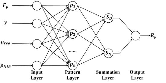
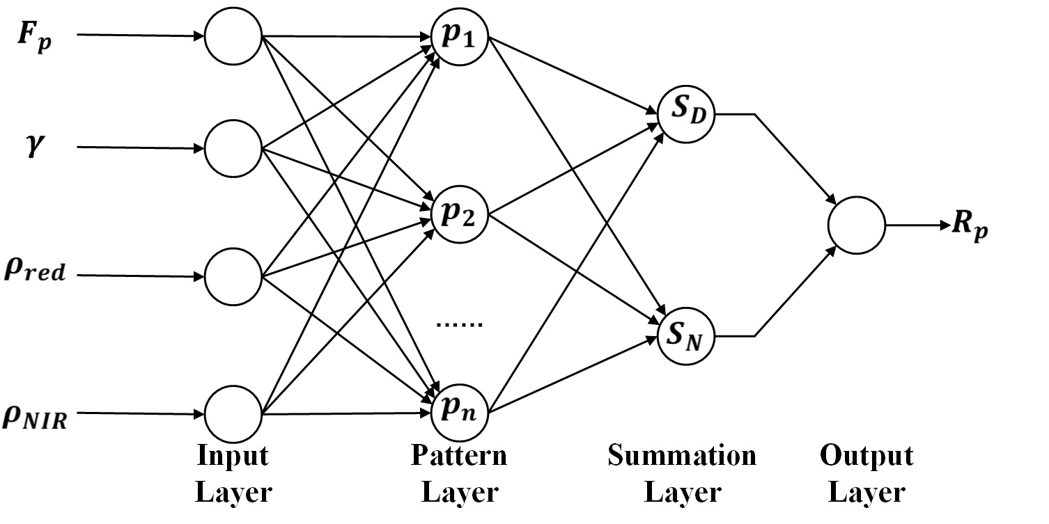
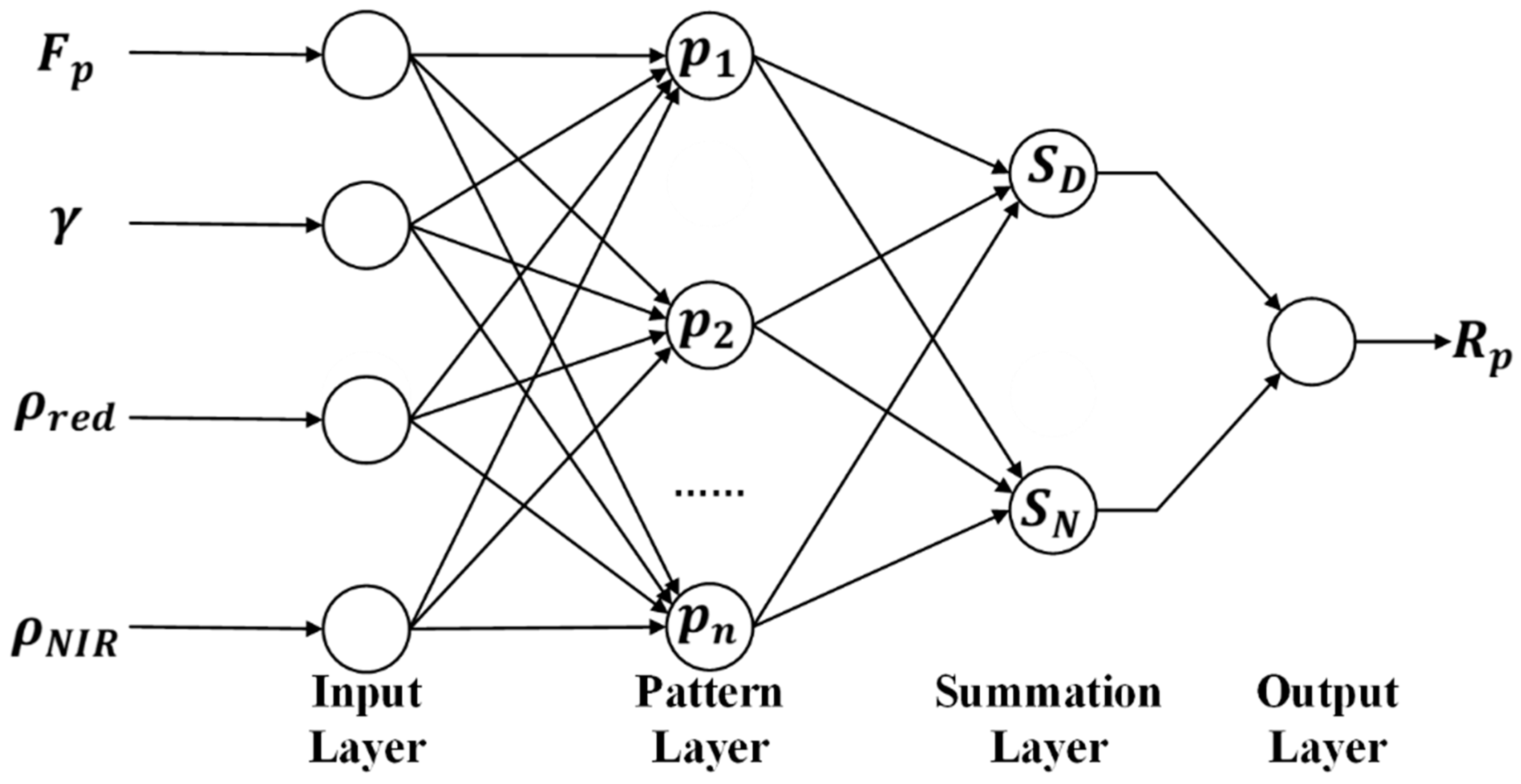
However, the joint PDF is generally unknown and must be estimated from the training dataset. To account for this problem, the GRNN designs four layers, namely the input, pattern, summation, and output layers (Figure 1). Detailed descriptions of the GRNN are given in [24]. Hereafter, we briefly introduce these four layers by incorporating the BPDF modeling of natural land surfaces.

The input layer gathers independent parameters into a 1-by-Q input vector, X. Here, Q is the number of independent parameters of the observation X. The polarized reflectance of a natural land surface has been reported to be a nonlinear function of the refractive index, sun-sensor geometry and/or vegetation coverage, as documented in [10,11]. The refractive index and the sun-sensor geometry can be parameterized by the Fresnel function ($F_p$) and the scattering angle ($\gamma$), whereas the vegetation coverage is related to the reflectances in the red (${\rho }_{red}$) and NIR (${\rho }_{NIR}$) bands [29]. We thus adopt the four parameters as the input independent parameters, $X=\left(F_p,\mathsf{\gamma },{\rho }_{red},{\rho }_{NIR}\right)$. In this case, X is a 1-by-4 vector (i.e., Q = 4).

The input vector is then passed on to the pattern layer, where the pattern function is calculated by using the input vector and a specific training observation $X_i$. Let n be the number of observations stored in the training dataset. Their difference is further fed into an exponential activation function using a smoothing parameter, $\sigma$. The smoothing parameter is actually the standard deviation of a Gaussian function. It controls the size of the GRNN receptive region. The pattern function $p_i$ can be derived from the following equation:

$$p_i=exp\left[-\frac{{\left(X-X_i\right)}^T\left(X-X_i\right)}{2{\sigma }^2}\right]\left(i=1,2,\dots ,n\right).$$

(6)

The summation layer performs two types of dot products ($S_D$ and $S_N$) between a weight vector and the pattern functions. The first product, $S_D$, is the simple sum of the pattern functions, i.e., every element in the weight vector equals to unity. The second product, $S_N$, is the sum of the pattern functions weighted by the corresponding polarized reflectance from the training observations, $Y$. The two types of dot products can be written as follows:

$$S_D={\displaystyle {{\displaystyle \sum }}_{i=1}^n}{p}_i,$$

(7)

$$S_N={\displaystyle {{\displaystyle \sum }}_{i=1}^n}{Y}_i{p}_i.$$

(8)

Finally, the output layer gives the conditional mean, $\widehat{Y}\left(X\right)$, by calculating the ratio between $S_N$ and $S_D$, i.e., $\widehat{Y}\left(X\right)=S_N/S_D$. In our case, $\widehat{Y}\left(X\right)$ is the estimated polarized reflectance ($R_p$) of the natural land surface corresponding to the independent vector X.

The four layers lay down the basics of the GRNN-based BPDF model. It is notable that the GRNN-based BPDF model includes only one free parameter, i.e., the smoothing parameter $\sigma$ (Equation (6)). The value of $\sigma$ impacts the performance of GRNN. When $\sigma \to \infty$, $\widehat{Y}\left(X\right)$ is close to the average of all the trained polarized reflectances. On the contrary, when $\sigma \to 0$, the estimated polarized reflectance from GRNN will be identical to the ground truth if the observation belongs to the training dataset; otherwise, unpredictable errors may occur if the observation does not exist in the training dataset. One thus must be careful in selecting the smoothing parameter, $\sigma$. For this purpose, we performed a cross-validation, which is described in the following subsection.

2.3. Cross-Validation

The cross-validation was performed to evaluate the accuracy of the GRNN-based BPDF model with different smoothing parameters and selected the one that provided the most accurate estimates, i.e., the RMSE between the validated and estimated polarized reflectance was minimized. Many cross-validation methods have been proposed thus far, such as the holdout, K-fold, and leave-one-out methods [24,30]. In this paper, given that the huge amount of training data, the K-fold method is selected.

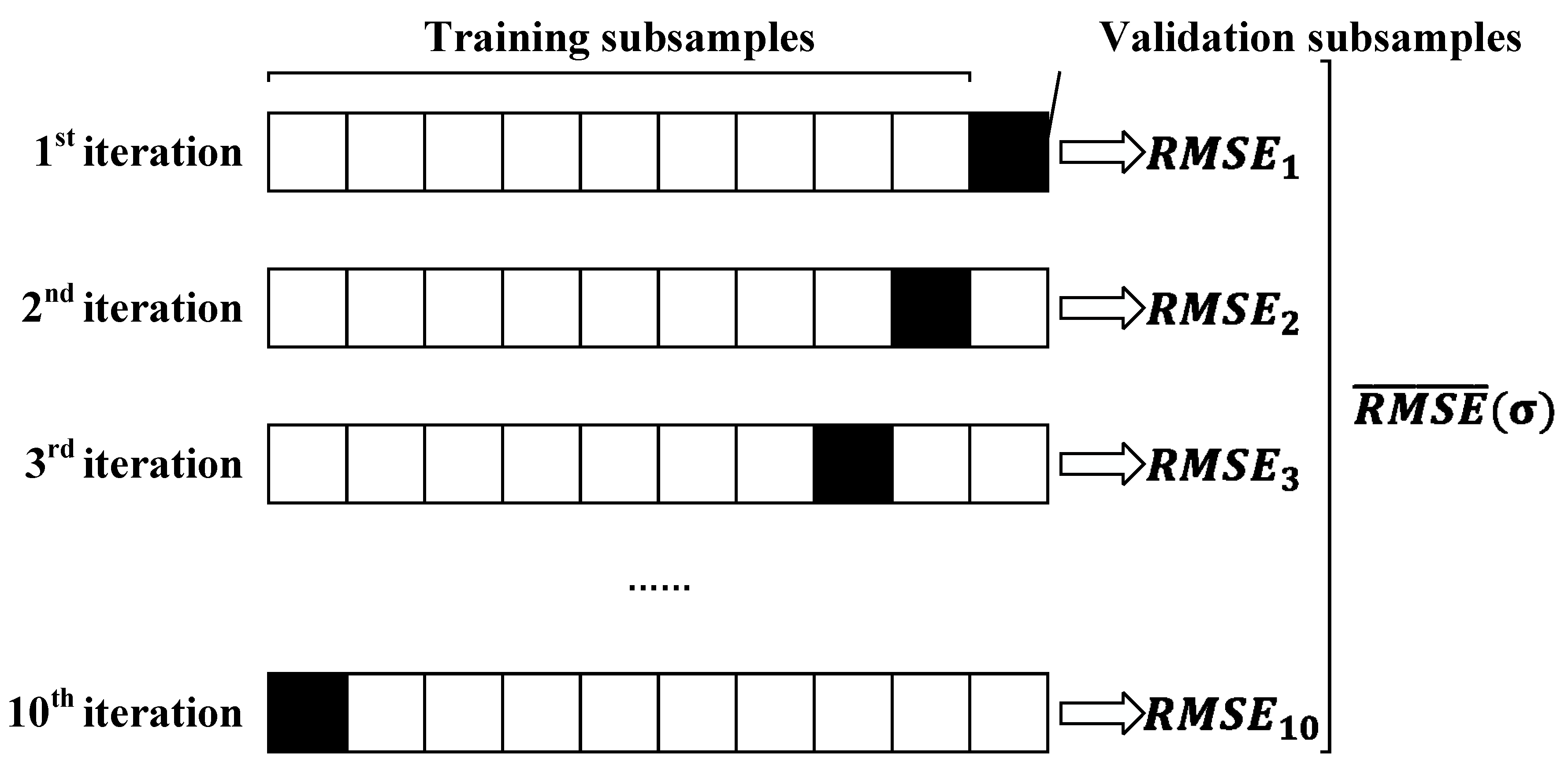
For a set of potential smoothing parameters, the K-fold method was designed as follows:

Step 1: The training dataset was randomly and equally divided into K subsamples;

Step 2: The GRNN-based BPDF model was executed by using a specific smoothing parameter, $\sigma$, with K-1 subsamples used as the training data, and the remaining one subsample used as the validation data;

Step 3: The RMSE between the estimated and the validated polarized reflectance was calculated;

Step 4: Steps 2 and 3 were repeated for K times, until each subsample had been used and only used once as the validation data, and $RMS{E}_1$, $RMS{E}_2$, …, and $RMS{E}_K$ were obtained;

Step 5: We calculated the average RMSE to quantify the accuracy of GRNN, i.e., $\overline{RMSE}\left(\sigma \right)=\frac{1}{K}{{\displaystyle \sum }}_{i=1}^{K}RMS{E}_i$, as illustrated in Figure 2;

Step 6: Steps 2–5 were then repeated with other smoothing parameters $\sigma$;

Step 7: Finally, we selected the smoothing parameter for which $\overline{RMSE}\left(\sigma \right)$ was the smallest.

In this paper, $K$ was set to 10. The selected $\sigma$ can further be used to estimate the polarized reflectance of natural land surfaces under any configuration of land surface type, refractive index, sun-sensor geometry and vegetation coverage.

2.4. Evaluation of the GRNN-Based BPDF Model

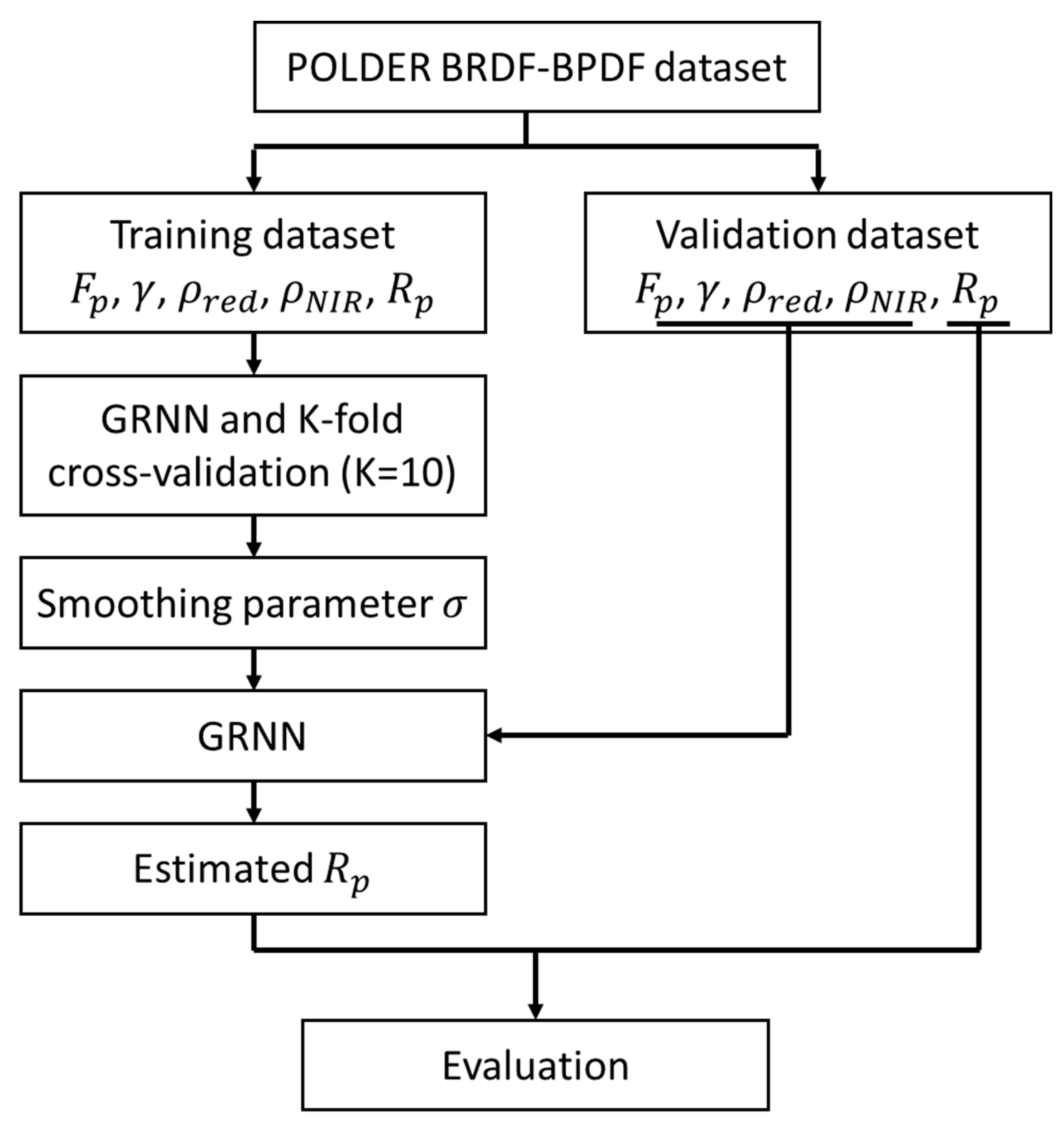
The procedure of evaluation of the GRNN-based BPDF model is presented in Figure 3. The approach can be described by the following steps:

Step 1: Divide the POLDER BRDF–BPDF dataset into two random equal parts, i.e., the training dataset and the validation dataset. Each dataset includes the Fresnel function, the scattering angle, reflectances at 670 and 865 nm, and the polarized reflectance.

Step 2: Use the GRNN-based BPDF model and K-fold cross-validation to select the smoothing parameter, $\sigma$, as described in Section 2.3.

Step 3: Run the GRNN-based BPDF model with the selected $\sigma$ and four input parameters (i.e., $F_p$, $\gamma$, ${\rho }_{red}$, and ${\rho }_{NIR}$) from the validation dataset to estimate the corresponding polarized reflectance of natural land surfaces.

Step 4: Compare the estimated polarized reflectance to the polarized reflectance stored in the validation dataset for evaluating the performance of the GRNN-based BPDF model.

3. Data

For this study, we used the official POLDER BRDF–BPDF database. The database was released in January 2017, and it remains the most accurate tool for the analysis of the polarization of light reflected by natural land surfaces [7]. Despite the fact that the POLDER radiometer collected a huge amount of measurements for over nine years, only a small group of surface targets with high-quality observations in the year of 2008 were selected for generating the database [7]. The top-of-atmosphere reflectance and polarized reflectance were atmospherically corrected to estimate the surface BRDF for six bands (0.490, 0.565, 0.670, 0.765, 0.865, and 1.020 $\mathsf{\mu }\mathrm{m}$) and estimate the surface BPDF at 0.865 $\mathsf{\mu }\mathrm{m}$. Note that the surface BPDF is only provided for a longer wavelength because, on one hand, the atmospheric correction is much more accurate than that at a shorter wavelength, and on the other hand, the surface BPDF is generally insensitive to the wavelength [4,28]. The calibration accuracy of the 865 nm polarized channel is about 0.5% [31]. The selected targets were organized into 16 classes using the International Geosphere–Biosphere Programme (IGBP) classification map. Each IGBP class included 50 targets for every month (i.e., 600 targets for every IGBP class).

The POLDER radiometer takes the scattering plane as a reference. The Stokes components (I, Q, and U), which are derived from three measurements through a polarizer with three orientations [32], are expressed with respect to the reference plane [7]. In this case, U is often negligible when compared to I and Q. Moreover, the measured polarization is often perpendicular to the reference plane (i.e., $Q<0$), and, only in rare cases the polarization is parallel to the reference plane (i.e., $Q>0$). The reflectance (R) and the polarized reflectance ($R_p$) are thus defined as follows:

$$R=\frac{\pi I}{E_{0}cos{\theta }_s},$$

(9)

$$R_p=\frac{-\pi Q}{E_{0}cos{\theta }_s}.$$

(10)

where ${\theta }_s$ represents the solar zenith angle (SZA), and $E_0$ is the top-of-atmosphere solar irradiance. With the above definitions, $R_p$ is generally positive but can be negative under some specific conditions. Both R and $R_p$ are functions of sun-sensor geometry. We use BRDF (or BPDF) to parameterize the angular distribution of R (or $R_p$).

Table 1. Information on selected targets.

ID	IGBP Class	Number of Targets	Mean Number of Observations
1	Evergreen needleleaf forests	564	72 ± 44
2	Evergreen broadleaf forests	551	61 ± 41
3	Deciduous needleleaf forests	536	67 ± 41
4	Deciduous broadleaf forests	595	72 ± 39
5	Mixed forests	581	69 ± 40
6	Closed shrublands	341	113 ± 49
7	Open shrublands	599	145 ± 55
8	Woody savannas	556	77 ± 47
9	Savannas	589	81 ± 51
10	Grasslands	599	118 ± 66
11	Permanent wetlands	553	60 ± 33
12	Croplands	575	102 ± 59
13	Urban and built-up	515	52 ± 34
14	Cropland/natural vegetation mosaics	572	70 ± 40
15	Snow and ice	554	374 ± 299
16	Barren or sparsely vegetated	597	171 ± 43

lists the statistic information on the selected targets used in this paper. It is notable that we excluded observations when either the polarized reflectances were unavailable (i.e., filled values in the POLDER BRDF-BPDF dataset) or the aerosol indication load was greater than 5. In addition, a target was also removed if all observations over it were excluded. Therefore, the number of selected targets for a given IGBP class was always less than 600 (Table 1). The number of selected observations for a given target also differed. The last column in Table 1 shows the mean number of selected observations ($\pm$ standard deviations).

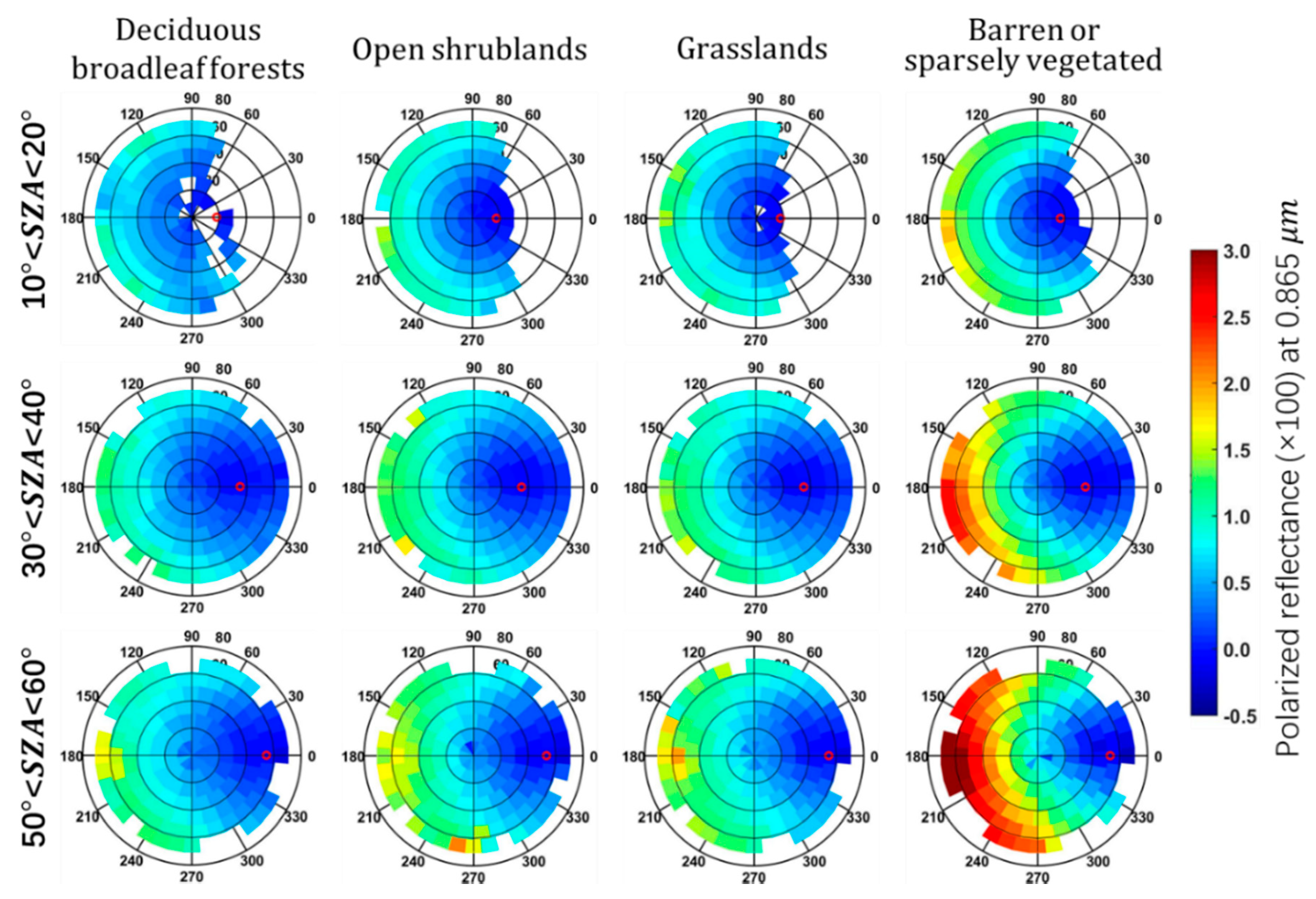
There are four IGBP classes whose number of selected targets were more than 590, i.e., deciduous broadleaf forests, open shrublands, grasslands, and barren or sparsely vegetated lands. These four classes were selected to represent the angular distributions of the measured polarized reflectance, which are shown in Figure 4. The measured polarized reflectance was highly anisotropic. It could be close to zero or even negative in backward scattering directions, and it could be up to a few percent (typically, less than 4%) in forward scattering directions. The polarized reflectance was generally symmetric about the principal plane. The hot-spot phenomenon, which often occurs for the reflectance of vegetation and soil, was not observed for the polarized reflectance. The angular distributions of the polarized reflectance for other IGBP classes were quite similar to the distributions shown in Figure 4. We thus do not show them in this paper.

4. Experiments and Results

The performance of the GRNN-based BPDF model was compared to six widely used models, i.e., Nadal–Bréon, Maignan, Waquet, Litivinov, Diner, and Xie–Cheng models. These models represent the most widely used models for modeling polarization of light reflected by natural land surfaces, as introduced in the Appendix A (

Table A1. Description on the six widely used semi-empirical BPDF models.

Models.	Formulas	Free Parameters	References
Nadal–Bréon	$R_p=\rho \left[1-\exp \left(-\beta \frac{F_p}{{\mu }_s+{\mu }_v}\right)\right]$	$\rho$, $\beta$	[9]
Waquet	$R_p=\xi ·F_p·S\left({\theta }_s\right)·S\left({\theta }_v\right)$ $S\left(\theta \right)=\frac{2}{1+\mathrm{erf}\left(\nu \right)+{\left(\nu \sqrt{\pi }\right)}^{-1}\exp \left(-{\nu }^2\right)}$ $\nu ={\left(\sigma \sqrt{2}\right)}^{-1}\tan \theta$	$\xi$, $\sigma$	[6]
Maignan	$R_p=\frac{C·\exp \left(-tan{\theta }_i\right)·\exp \left(-NDVI\right)·F_p}{4\left({\mu }_s+{\mu }_v\right)}$	C	[10]
Litvinov	$R_p=\frac{\alpha \pi F_p}{4\cos \vartheta \left({\mu }_s+{\mu }_v\right)}f\left(\sigma ,\vartheta \right)f_{sh}\left(\gamma ,k_r\right)$ $f\left(\sigma ,\vartheta \right)=\frac{1}{\pi {\cos }^3\vartheta ·2{\sigma }^2}\exp \left(-\frac{{\tan }^2\vartheta }{2{\sigma }^2}\right)$ $\cos \vartheta =\frac{{\mu }_s+{\mu }_v}{2{\mu }_i}$ $f_{sh}\left(\gamma ,k_r\right)={\left(\frac{1+cos{k}_r\left(\pi -\gamma \right)}{2}\right)}^3$	$\alpha$, $\sigma ,$$k_r$	[18]
Diner	$R_p=\frac{\xi F_p}{8\pi {\mu }_s{\mu }_v\cos \vartheta }$	$\xi$	[17]
Xie–Cheng	$R_p=A·F_p·f_{sh}\left(\gamma ,k_r\right)·\exp \left(-0.7·NDVI\right)$	$A,k_r$	[11]

) and as documented in [4,10,11]. We compared these models from two aspects: one for data collected during the whole year, and the other for data collected during every single month.

4.1. Comparison Using Data Collected during the Whole Year

These models were compared by using data collected during the whole year, which included <600 targets for each IGBP class, as presented in Table 1. For a given IGBP class, the evaluation process for the GRNN-based BPDF model followed Figure 3. For the other six BPDF models, the training dataset was used for retrieving free parameters, whereas the validation dataset was adopted for evaluating the performance of these models using free parameters adjusted from the training dataset. The RMSE between measured and modeled polarized reflectance was used for comparison.

Table 2. RMSEs between modeled and measured polarized reflectance. The values in bold have the smallest RMSE for a given International Geosphere–Biosphere Programme (IGBP) class. All values presented have been multiplied by a factor of 100.

IGBP ID	Nadal–Bréon Model	Maignan Model	Waquet Model	Litvinov Model	Diner Model	Xie–Cheng Model	GRNN–Based Model
1	0.313	0.315	0.334	0.322	0.405	0.317	0.256
2	0.220	0.225	0.240	0.224	0.322	0.222	0.219
3	0.392	0.386	0.447	0.393	0.527	0.418	0.324
4	0.255	0.251	0.297	0.260	0.364	0.261	0.224
5	0.250	0.249	0.274	0.255	0.334	0.255	0.226
6	0.142	0.172	0.180	0.145	0.324	0.141	0.110
7	0.180	0.195	0.216	0.186	0.379	0.178	0.129
8	0.242	0.246	0.269	0.246	0.341	0.243	0.224
9	0.231	0.243	0.268	0.235	0.362	0.233	0.186
10	0.235	0.243	0.280	0.244	0.425	0.238	0.174
11	0.356	0.367	0.381	0.358	0.457	0.377	0.275
12	0.231	0.233	0.278	0.241	0.436	0.236	0.221
13	0.255	0.267	0.278	0.269	0.446	0.253	0.256
14	0.261	0.264	0.305	0.271	0.449	0.265	0.256
15	0.459	0.481	0.561	0.507	0.751	0.484	0.405
16	0.171	0.182	0.204	0.180	0.372	0.171	0.144
Avg	0.262	0.270	0.301	0.271	0.418	0.268	0.227

presents the RMSEs for every model and every IGBP class. The values in bold correspond to the smallest RMSE for a given IGBP class. The GRNN-based BPDF model had the smallest RMSEs for 15 IGBP classes. Only for one IGBP class, i.e., IGBP 13 (urban and built-up), the GRNN-based BPDF model (RMSE = 0.256%) was slightly worse than the Xie–Cheng model (RMSE = 0.253%), which was designed for IGBP 13. The adjusted smoothing parameters for the 16 IGBP classes are presented in

Table 3. Selected smoothing parameters (σ).

IGBP ID	$\mathit{\sigma }$	IGBP ID	$\mathit{\sigma }$
1	0.11	9	0.04
2	0.04	10	0.05
3	0.06	11	0.07
4	0.07	12	0.05
5	0.06	13	0.25
6	0.04	14	0.08
7	0.03	15	0.02
8	0.04	16	0.03

.

We also calculated the averaged RMSEs of 16 IGBP classes for each model, as presented in the last row of Table 2. The Nadal–Bréon, Maignan, Litivinov, and Xie–Cheng models are the best current models because they all achieve comparable and generally satisfactory average RMSE, i.e., 0.262%, 0.270%, 0.271%, and 0.268%, respectively. The Waquet and Diner models were the relatively worse performers, with an average RMSE equal to 0.301% and 0.418%, respectively. The GRNN-based BPDF model had the smallest average RMSE (0.227%). Compared to these best current models, the GRNN-based BPDF model reduced the average RMSE by >13.4% (= (0.262 − 0.227)/0.262). It is thus clear that the GRNN-based BPDF model performed best among these models using data collected during the whole year.

The above comparison followed the standard technique descripted in [10]. It assumes that the optical properties of a given IGBP class do not change throughout the year. However, this may not be the case in reality, i.e., the optical properties of the 16 IGBP classes may change monthly. Our next step was to evaluate these models using data collected during every single month.

4.2. Comparison Using Data Collected during Every Single Month

The evaluation process used here is quite similar to that presented in Section 4.1. The only difference is that, for a given IGBP class, rather than using the observations collected during the whole year, we used the observations collected during every single month, independently. Therefore, the RMSE was calculated for each IGBP class and each month. These RMSEs were compared for evaluation of the models under the case that the optical properties of land surfaces may change throughout the year.

Figure 5 illustrates the difference between the RMSE obtained from the GRNN-based BPDF model and that from the other six models for 192 cases (i.e., for 16 IGBP classes and 12 months). The negative values mean that the RMSE obtained from the GRNN-based BPDF model was smaller than that from the compared model, indicating that the GRNN-based BPDF model was more accurate. As one can see from the top-left panel in Figure 5, the GRNN-based BPDF model was more accurate than the Nadal–Bréon model in 188 cases (out of 192 cases, 188/192 = 97.9%). In only four cases, the RMSE obtained from the Nadal–Bréon model was smaller than that from the GRNN-based BPDF model. Moreover, the difference was very small (less than 0.04%). Similar results were found when the GRNN-based BPDF model was compared to the Maignan, Waquet, Litvinov, Diner, and Xie–Cheng models (Figure 5), i.e., the GRNN-based BPDF model was more accurate in 187 (97.4%), 191 (99.5%), 189 (98.4%), 192 (100%), and 188 (97.9%) cases, respectively. These results confirm that the GRNN-based BPDF model is more accurate than the other models when using data collected during every single month.

5. Discussion

Solar radiation scattered by natural land surfaces is partly polarized. Polarization of light reflected by natural land surfaces was found to be a nonlinear function of three factors, i.e., refractive index, sun-sensor geometry, and/or vegetation coverage [4,11]. GRNN showed a good ability of nonlinear approximation. In this study, we thus developed a GRNN-based BPDF model. In order to simplify the modeling process, we did not directly use refractive index, sun-sensor geometry, and vegetation coverage as input parameters because; on one hand, the GRNN-based BPDF model requires too many input parameters, on the other hand, the vegetation coverage is neither provided by the POLDER BRDF–BPDF dataset nor easy to be retrieved from the dataset. Therefore, four parameters, i.e., Fresnel factor (Equation (4)), scattering angle (Equation (1)), red and NIR reflectances, which are closely related to the three above factors, were used as the input parameters for the GRNN-based BPDF model (Equations (5)–(8)). We also analyzed several more groups of input parameters by adding some other available parameters, such as vegetation indices and/or reflectance at other bands. However, the addition of these parameters did not increase the accuracy of the GRNN-based BPDF model very much while they made it much more computationally intensive during the training process. We thus opted for not including any other parameters in addition to the four input parameters.

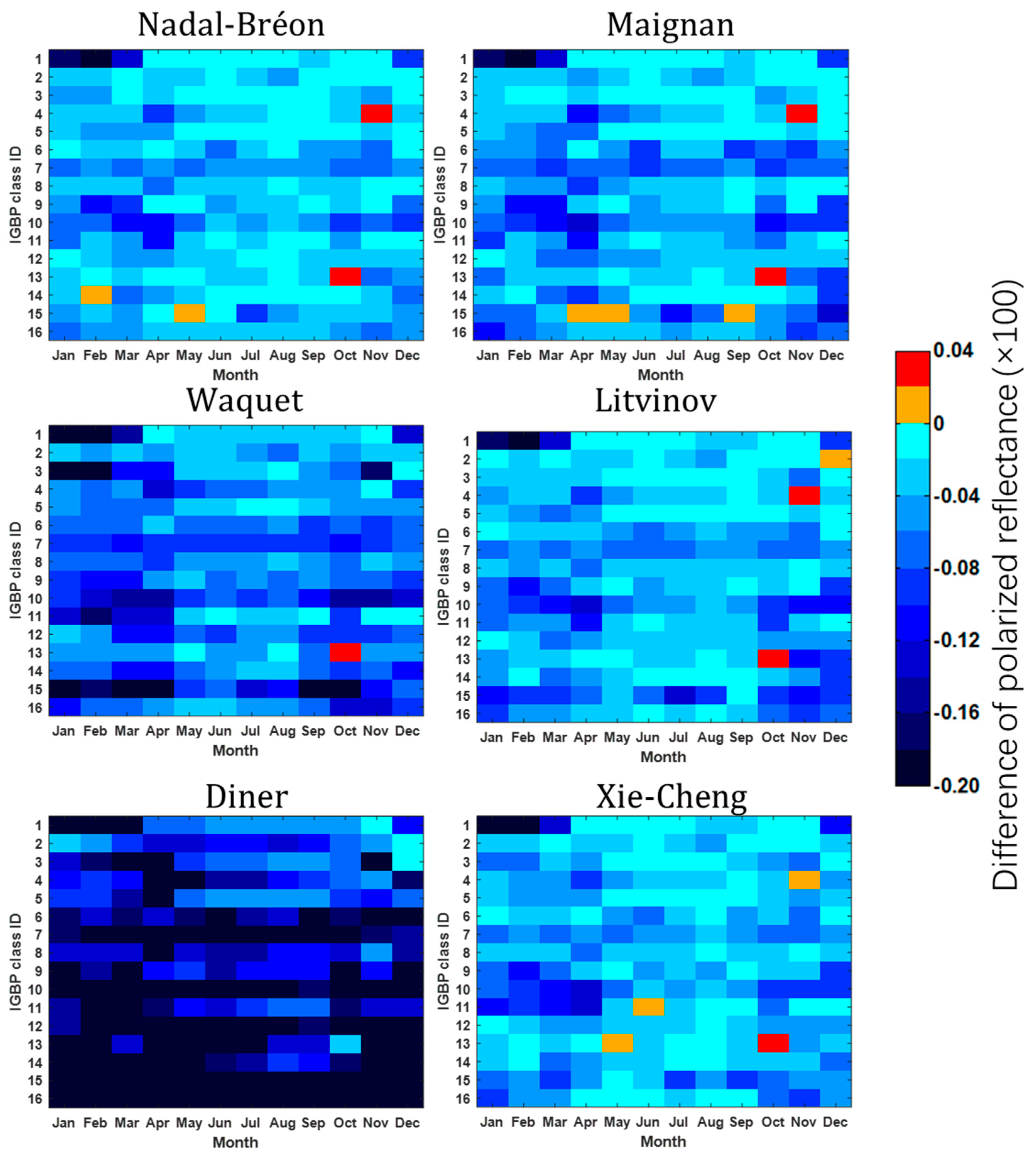
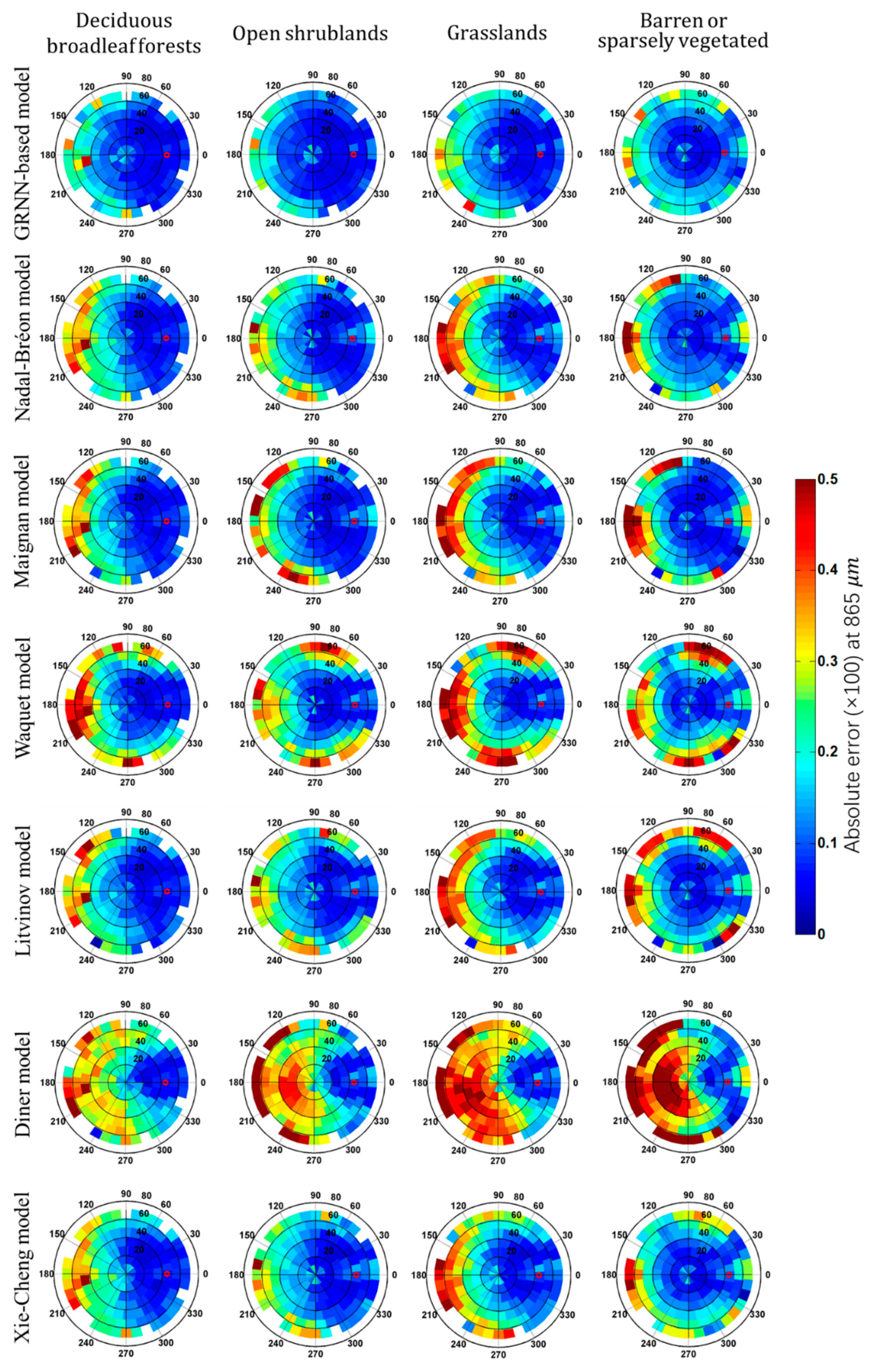
The performance of the GRNN-based BPDF model (Figure 3) was evaluated using the POLDER BRDF–BPDF dataset through comparisons with six widely used BPDF models. Our experiments confirmed a better performance of the GRNN-based BPDF model compared to the six BPDF models both when using data collected during the whole year (Table 2) and every single month (Figure 5). Figure 6 illustrates the absolute error distribution using observations collected during the whole year and with SZA ranging between $40°$ and $50°$. Figure 6 shows that the largest absolute error appeared in forward scattering directions. The polarized reflectance is usually large when the scattering angle is small. Therefore, it is sensitive to the optical properties of the land surfaces, i.e., a small change in optical properties may cause a great difference in the polarized reflectance. The six widely used models cannot capture these changes and thus introduce greater absolute errors. The GRNN-based BPDF model provides a complicated nonlinear relationship between polarized reflectance and inputs. The changes can be accurately captured by the joint PDF. The GRNN-based BPDF model is thus accurate even when the scattering angle is small. It also performs better in other view directions, as Figure 6 illustrates. Therefore, the results suggest that the GRNN-based BPDF model provides the best estimates in almost every view direction.

Another advantage of the GRNN-based BPDF model is its ability to reproduce the negative polarized reflectance. Due to coherent backscattering and shadowing [33,34], the polarized reflectance can be negative (i.e., the polarization of light reflected by natural land surfaces is parallel to the scattering plane, see Equation (10)) in the backscattering direction. However, the existing BPDF models assume a positive polarized reflectance and thus the modeled polarized reflectance is always greater than or equal to zero. The GRNN-based BPDF model allocates the sum of all training sample probabilities [24] and thus can reproduce negative polarized reflectance. 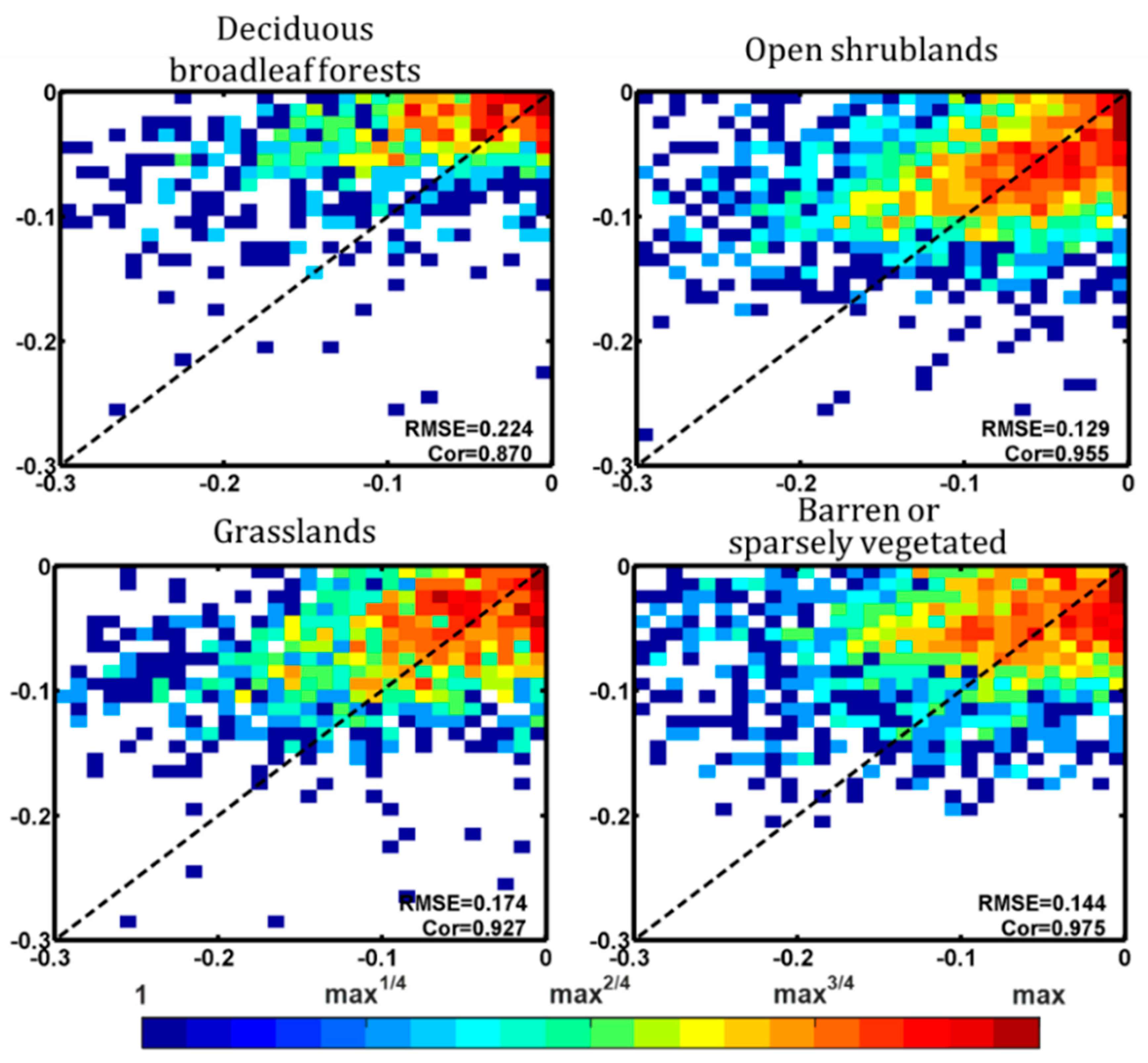Figure 7 shows the correlation between modeled and measured polarized reflectance for deciduous broadleaf forest, open shrublands, grasslands, and barren or sparsely vegetated lands. Note that the color of each bin represents the logarithmic value of the number of observations, indicating that a red bin has much more observations than that of a blue bin. Generally, the RMSEs for the four IGBP classes are small (less than 0.224%) and the correlations are apparent (greater than 0.870). However, the GRNN-based BPDF model slightly overestimated the negative polarized reflectance (Figure 7). This was expected, because the negative polarized reflectance is close to zero (generally greater than −0.003) and only exists within a small view region; the estimated negative polarized reflectance can be affected by its nearby positive polarized reflectance. More datasets collected from different sensors could be helpful for further validation of the GRNN-based model. Nevertheless, the GRNN-based BPDF model is the first model that can reproduce the negative feature.

A potential criticism of the GRNN-based BPDF model is the spatial resolution of the POLDER measurements, limited to $\approx 6.2\times 6.2{\mathrm{km}}^2$ [35]. One may argue that the resolution is so low that the GRNN-based BPDF model cannot be applied to a finer scale. Actually, only a POLDER pixel for which >75% of the pixel was covered by a given land-cover type was selected for generating the BRDF–BPDF database [7]. The POLDER pixel is quite homogenous and thus the spatial resolution is not a critical issue. Besides, different land covers, such as deciduous broadleaf forest and grassland, have shown similar angular distributions of the polarize reflectance (Figure 4), indicating that the canopy structure has negligible impact [10]. Therefore, one can expect that the GRNN-based BPDF model can be applied to a finer scale.

Another potential criticism of the GRNN-based BPDF model is the atmospheric correction of the POLDER measurements. One may question that the POLDER BRDF–BPDF database does not really provide the polarization of light reflected by natural land surfaces because the database was not corrected for aerosol scattering [7]. To minimize the impact of the aerosol scattering, only a POLDER pixel for which the aerosol indication load was not greater than 5 was selected in this study. Here, the aerosol indication load varies between 0 (a low aerosol load) and 15 (a high aerosol load) [7]. Therefore, the POLDER pixels used in this study were collected during quite clear days, and the impact of the aerosol scattering was minimized.

The GRNN-based BPDF model has only one free parameter, i.e., the smoothing parameter. This parameter can be accurately adjusted using the K-fold cross-validation method (Figure 2). The GRNN-based BPDF model, together with the well-trained smoothing parameter (Table 3) and four input parameters, can be used for estimation of polarized reflectance of natural land surface under any configuration of land surface type, refractive index, sun-sensor geometry and vegetation coverage.

BPDF models are mainly used for retrieval of aerosol properties (e.g., aerosol optical depth (AOD)). The accuracy of the POLDER polarization measurements at 865 nm is lower than 0.01 in RMSE [11]. Typically, an error of 0.1% for the polarized reflectance of natural land surfaces leads to an error of 4% on AOD [10]. According to Table 2 and Figure 5, the RMSE difference between the GRNN-based BPDF model and the best current BPDF models varies with land-cover type (ranging from 0.001% (IGBP 2) to 0.081% (IGBP 11)), indicating that the error of AOD can be up to 3.24%, which is larger than the acceptable AOD retrieval error required by the climate research over land [6,36]. In addition, a more accurate BPDF model is needed for the simultaneous retrieval of AOD and aerosol microphysical properties [11]. Thus, one may expect that the GRNN-based BPDF model can be useful in climate research and remote sensing of complete aerosol properties over land [37,38].

6. Conclusions

Modeling polarized reflectance of natural land surfaces has been a hot topic in the past two decades, especially after the launch of the POLDER radiometer. Six BPDF models have been proposed, i.e., Nadal–Bréon, Maignan, Waquet, Litivinov, Diner and Xie–Cheng models. All of these widely used models indicate that the polarized reflectance of natural land surfaces is a nonlinear function of variables related to refractive index, sun-sensor geometry, and/or vegetation coverage. While the GRNN is suitable for solving nonlinear problems, it has never been used in the modeling of the polarized reflectance of natural land surfaces. To overcome this gap, this paper proposed a GRNN-based BPDF model. Four parameters, i.e., Fresnel factor, scattering angle, red and NIR reflectances, were selected as the neural network inputs. The GRNN-based BPDF model displayed good abilities on fast learning because only one free parameter, i.e., the smoothing parameter, needs to be adjusted. The GRNN-based BPDF model is the most accurate, as, on one hand, it works well even when the scattering angle is small; and on the other hand, it is the first model able to reproduce negative polarized reflectances. Overall, compared to the best current BPDF models, it can reduce the average RMSE by 13.4% with data collected during the whole year, and its RMSE is lower for 97.4% cases with data collected during every month.

This paper provided an alternative solution for modeling the polarization of light reflected by natural land surfaces. The GRNN-based BPDF model can be applied to research on complete aerosol parameter retrieval as boundary condition. Note that, with the development of machine learning, there may be many other neural networks that could provide even better performance than the GRNN. This paper verified the possibility of using machine learning in modeling of polarization of light reflected by natural land surfaces. Moreover, although the GRNN-based BPDF model was validated by using the POLDER measurements, the four input parameters are quite straightforward and can be easily collected by any remote sensing radiometer, thus allowing us to extend the approach to further studies of polarized measurements of GF-5 [39], 3 MI [40], SGLI [41], and CAPI [42] etc.