Article

A Coarse-to-Fine Network for Ship Detection in Optical Remote Sensing Images

1
Key Laboratory of Big Data and Intelligent Vision, School of Computer Science and Technology, Xidian University, Xi’an 710071, China
2
Key Laboratory of Intelligent Perception and Image Understanding of Ministry of Education, School of Articial Intelligence, Xidian University, Xi’an 710071, China
3
School of Electronic Engineering, Key Laboratory of Intelligent Perception and Image Understanding of Ministry of Education, Xidian University, Xi’an 710071, China
*
Author to whom correspondence should be addressed.
Remote Sens. 2020, 12(2), 246; https://doi.org/10.3390/rs12020246
Submission received: 20 November 2019 / Revised: 25 December 2019 / Accepted: 27 December 2019 / Published: 10 January 2020

Abstract

:
With the increasing resolution of optical remote sensing images, ship detection in optical remote sensing images has attracted a lot of research interests. The current ship detection methods usually adopt the coarse-to-fine detection strategy, which firstly extracts low-level and manual features, and then performs multi-step training. Inadequacies of this strategy are that it would produce complex calculation, false detection on land and difficulty in detecting the small size ship. Aiming at these problems, a sea-land separation algorithm that combines gradient information and gray information is applied to avoid false alarms on land, the feature pyramid network (FPN) is used to achieve small ship detection, and a multi-scale detection strategy is proposed to achieve ship detection with different degrees of refinement. Then the feature extraction structure is adopted to fuse different hierarchical features to improve the representation ability of features. Finally, we propose a new coarse-to-fine ship detection network (CF-SDN) that directly achieves an end-to-end mapping from image pixels to bounding boxes with confidences. A coarse-to-fine detection strategy is applied to improve the classification ability of the network. Experimental results on optical remote sensing image set indicate that the proposed method outperforms the other excellent detection algorithms and achieves good detection performance on images including some small-sized ships and dense ships near the port.

1. Introduction

Ship detection in optical remote sensing image is a challenging task and has a wide range of applications such as ship positioning, maritime traffic control and vessel salvage [1]. Differing from natural image that taken in close-range shooting with horizontal view, remote sensing image acquired by satellite sensor with a top-down perspective is vulnerable to the factor such as weather. Offshore and inland river ship detection has been studied on both synthetic aperture radar (SAR) and optical remote sensing imagery. Some alternative methods of machine learning approaches have also been proposed [2,3,4,5]. However, the classic ship detection methods based on SAR images will cause a high false alarm ratio and be influenced by the sea surface model, especially on inland rivers and in offshore areas. Schwegmann et al. [6] used deep highway networks to avoid the vanishing gradient problem. They developed their own three-class SAR dataset that allows for more meaningful analysis of ship discrimination performances. They used data from Sentinel-1 (Extra Wide Swath), Sentinel-3 and RADARSAT-2 (Scan-SAR Narrow). They used Deep Highway Networks 2, 20, 50, 100 with 5-fold cross-validation and obtained an accuracy of 96% outperforming classical techniques such as SVM, Decision Trees, and Adaboost. Carlos Bentes et al. [7] used a custom CNN with TerraSAR-X Multi Look Ground Range Detected (MGD) images to detect ships and iceberg. They compared their results with SVM and PCA+SVM, and showed that the proposed model outperforms these classical techniques. The classic detection methods based on SAR images do not perform well on small and gathering ships. And with the increasing resolution and quantity of optical remote sensing images, ship detection in optical remote sensing images has attracted a lot of research interests.This paper mainly discusses ship detection in optical remote sensing images. In the object detection task, natural image is mainly used to front-back object detection. By contrast, remote sensing image is mainly used to left-right object detection [8]. Ship detection in remote sensing image is immensely affected by the viewpoint changes, cloud occlusion, wave interference, background clutter. Of these, the characteristics of optical remote sensing image such as the diversity of target size, high complexity of background and small targets makes ship detection particularly difficult.
In recent years, ship detection methods in optical remote sensing image mainly adopt a coarse-to-fine detection strategy which is based on two-stage [9,10]. The first step is the ship candidate extraction stage. All candidate regions that possibly contain ship targets are searched out in the entire image by some region proposal algorithms, which is a coarse extraction process. In this case, the information of image such as color, texture and shape is usually taken into account [1,11]. Region proposal algorithms include the sliding windows-based method [12], the image segmentation-based method [10], and the saliency analysis-based method [13,14]. These methods can preliminarily extract the candidate region of ships, then the ship candidate region is filtered and merged according to shape, scale information and neighborhood analysis methods [15]. Selective search algorithm (SS) [16] is a representative algorithm for candidate region extraction and is widely used in object detection task.
The second step is the ship recognition stage. The ship candidate regions are classified by a binary classifier which distinguishes whether the ship target is located in the candidate region [17]. It is a fine recognition process. The features of ships are extracted and then candidate regions are classified. Many traditional methods extract low-level features, such as scale-invariant feature transform (SIFT) [18], histogram of oriented gradients (HOG) [19], deformed part mode (DPM) feature [20] and structure-local binary patterns (LBP) feature [21,22] to classify candidate regions. With the popularization of deep learning, some methods use convolution neural network (CNN) to extract the features of ships, which are the high-level feature with more semantic information. These extracted features combine with a classifier to classify all candidate regions to distinguish the ship from the background. Many excellent classifiers such as the support vector machine (SVM) [1,23], AdaBoost [24], and unsupervised discrimination strategy [13] are adopted to recognize the candidate regions.
Although the traditional method has achieved considerable detection results in clear and calm ocean environments, there still have many deficiencies. Yao et al. [25] found that the traditional methods have some shortcomings. First, the extracted candidate regions have a large amount of redundancy, which leads to expensive calculation. Second, the manual feature focuses on the shape or texture of ships, which requires manual observation of all ships. The complex background and variability in ship size will lead to poor detection robustness and low detection speed. Most important of all, when the size of the ships is very small or the ships are concentrated at the port, the extraction of the ship candidate region is particularly difficult. Therefore, the accuracy and efficiency of ship detection are greatly reduced.
Recently, convolutional neural networks (CNN) with good feature expression capability have widely used in image classification [26], object detection [27,28], semantic segmentation [29], image segmentation [30], image registration [31,32]. Object detection based on deep convolution neural network has achieved good performance on large scale natural image data set. These methods are mainly divided into two main categories: two-stage method and one-stage method. Two-stage method originated from R-CNN [33], then successively arise Fast R-CNN [34] and Faster R-CNN [28]. R-CNN is the first object detection framework based on deep convolutional neural networks [35], which uses the selective search algorithm (SS) to extract the candidate regions and computes features by CNN. A set of class-specific linear SVMs [36] and regressors are used to classify and fine-tune the bounding boxes, respectively. Fast R-CNN is improved on the basis of R-CNN to avoid repeated calculations of candidate region features. Faster R-CNN proposes a region proposed network (RPN) instead of the selective search method (SS) to extract candidate regions, which improves the computational efficiency by sharing the features between the RPN and the object detection network. One-stage methods, such as YOLO [27] and SSD [37], solve the detection problem as a regression problem and achieve an end-to-end mapping directly from image pixels to bounding box coordinates by a full convolutional network. SSD detects objects on multiple feature maps with different resolutions from a deep convolutional network and achieves better detection results than YOLO.
In recent years, many ship detection algorithms [25] based on deep convolutional neural networks have been proposed. These methods intuitively extract features of images through CNN, avoiding complex shape and texture analysis, which significantly improve the detection accuracy and efficiency of ships in optical remote sensing images. Zhang et al. [38] proposed S-CNN, which combines CNN with the designed proposals extracted from two ship models. Zou et al. [23] proposed the SVD Networks, which use CNN to adaptively learn the features of the image and adopt feature pooling operation and the linear SVM classifier to determine the position of the ship. Hou et al. [39] proposed the size-adapted CNN to enhance the performance of ship detection for different ship sizes, which contains multiple fully convolutional networks of different scales to adapt to different ships sizes. Yao et al. [25] applied a region proposal network (RPN) [28] to discriminate ship targets and regress the detection bounding boxes, in which the anchors are designed by intrinsic shape of ship targets. Wu et al. [40] trained a classification network to detect the locations of ship heads, and adopted an iterative multitask network to perform bounding-box regression and classification [41]. But these methods must first perform feature region extraction operations, so the efficiency of the algorithm is reduced. The most important is that these methods can produce more false detection on land and small ship cannot be detected.
This paper includes three main contributions:
(1) Aiming at the false detection on land, we use a sea-land separation algorithm [42] which combines gradient information and gray information. This method uses gradient and gray information to achieve preliminary separation of land and sea, and then eliminates non-connected regions through a series of morphological operations and ignoring small area operations.
(2) About small ship cannot be detected, we used The Feature Pyramid Network (FPN) [43] and a multi-scale detection strategy to solve this problem. The Feature Pyramid Network (FPN) proposes a top-down path that combines a horizontally connected structure that combines low resolution, strong semantic features with high resolution, weak semantic features to effectively solve small target detection problem. The multi-scale detection strategy is proposed to achieve ship detection with different degrees of refinement.
(3) We designed a two-stage inspection network for ship detection in optical remote sensing images. It can obtain the position of the predicted ship directly from the image without additional candidate region extraction operations, which greatly improves the efficiency of ship detection. Finally, we propose a coarse-to-fine ship detection network (CF-SDN) which has the feature extraction structure with the form of feature pyramid network, achieving end-to-end mapping directly from image pixels to bounding boxes with confidence scores. The CF-SDN contains multiple detection layers with a coarse-to-fine detection strategy employed at each detection layer.
The remainder of this paper is organized as follows. In Section II, we introduce our method including procedure of optical remote sensing image preprocessing including the sea-land separation algorithm, the multi-scale detection strategy, two strategies to eliminate the influence of cutting image, and the structure of the coarse-to-fine ship detection network (CF-SDN), including the feature extraction structure, the distribution of anchor, the coarse-to-fine detection strategy, the details of training and testing.. Section III describes the experiments performed on optical remote sensing image data set and Section IV presents conclusions.

2. Methodology

In this section, we will introduce the procedure of optical remote sensing image preprocessing including the sea-land separation algorithm, the multi-scale detection strategy, two strategies to eliminate the influence of cutting image, and the structure of the coarse-to-fine ship detection network (CF-SDN), including the feature extraction structure, the distribution of anchor, the coarse-to-fine detection strategy, the details of training and testing. The procedure of optical remote sensing image preprocessing is shown in Figure 1.

2.1. Sea-land Separation Algorithm

Optical remote sensing images are obtained by satellites and aerial sensors. So the area that the image covered is wide and the geographical background is complex. In ship detection task, ships are usually scattered in water area (sea area) or in inshore area. In generally, the land and ship area present a relatively high gray level and have much complex texture, which are contrary to the situation in the sea area. Due to the complexity of the background in optical remote sensing images, the characteristics of some land areas are very similar to those of ships. This can easily lead to the detection of ship on land, which is called false alarm. Therefore, it is necessary to use sea-land separation algorithms to distinguish the sea area (or water area) from the land area before formal detection.
The sea-land separation algorithm [42] used in this paper considers the gradient information and the gray information of the optical remote sensing image comprehensively, combines some typical image morphology algorithms, and finally generates a binary image. In the process of sea-land separation, the algorithm that only considers the gradient information of the image performs well when the sea surface is relatively calm and the land texture is complex. However, the algorithm is difficult to achieve sea-land separation when the sea surface texture is complicated. The algorithm considering gray-scale information of the image is suitable for processing uniform texture images, but is difficult to process a complex image region. Therefore, the advantages of these two algorithms can be complemented with each other. The combination of gradient information and gray scale information can adapt to the complex situation of the optical remote sensing images, and can overcome the problem of poor sea-land separation performance caused by considering single information. The sea-land separation process is shown in Figure 2. The specific implementation details of the algorithm are as follows:
(1) Threshold segmentation and edge detection are performed on the original image respectively. Before the threshold segmentation, the contrast of the image is enhanced to highlight the regions where the pixel values have large difference. Similarly, the image should be smoothed before performing edge detection. The traditional edge detection methods produce a lot of subtle wavy textures on the sea surface, which can be eliminated by filters. Here, we enhance the contrast of the image by histogram equalization, and perform threshold segmentation by the Otsu algorithm. At the same time, the median filter is used to smooth the image and the median filter size that selected in our experiment is 5 × 5 , because the median filter is a nonlinear filtering that can not only remove noise but also preserve the edge information of the image when the image background is complex. Then the canny operator is used to detect the image edges, and we set the low and high thresholds to 10% of the maximum and 20% of the maximum, respectively.
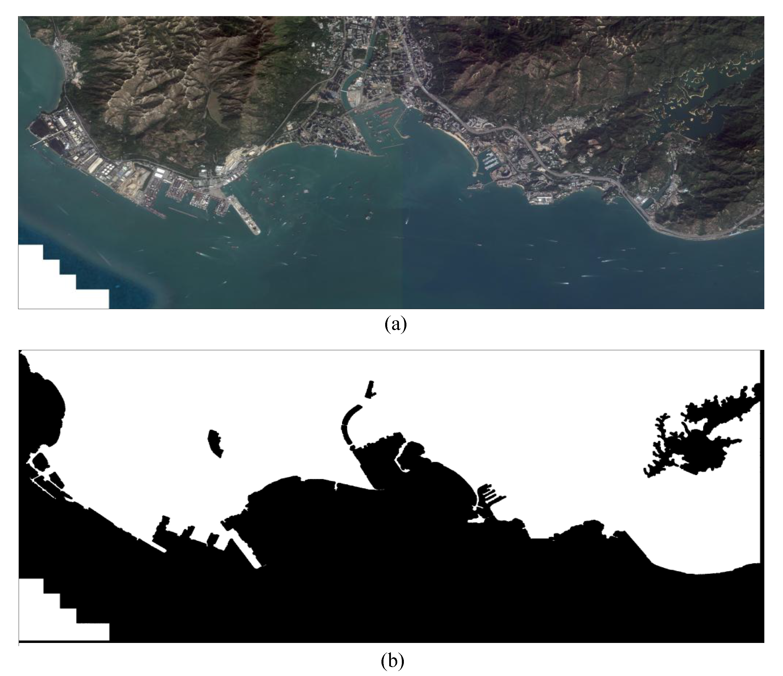
(2) The threshold segmentation results and the edge detection results are combined by logical OR operation, then a binary image is generated to highlight non-water areas, which is regarded as the preliminary sea-land separation result. In the binary image, The pixel value of the land area is set to 1, and the pixel value of the water area is set to 0. The final result (such as IMAGES3) is shown in Figure 3.
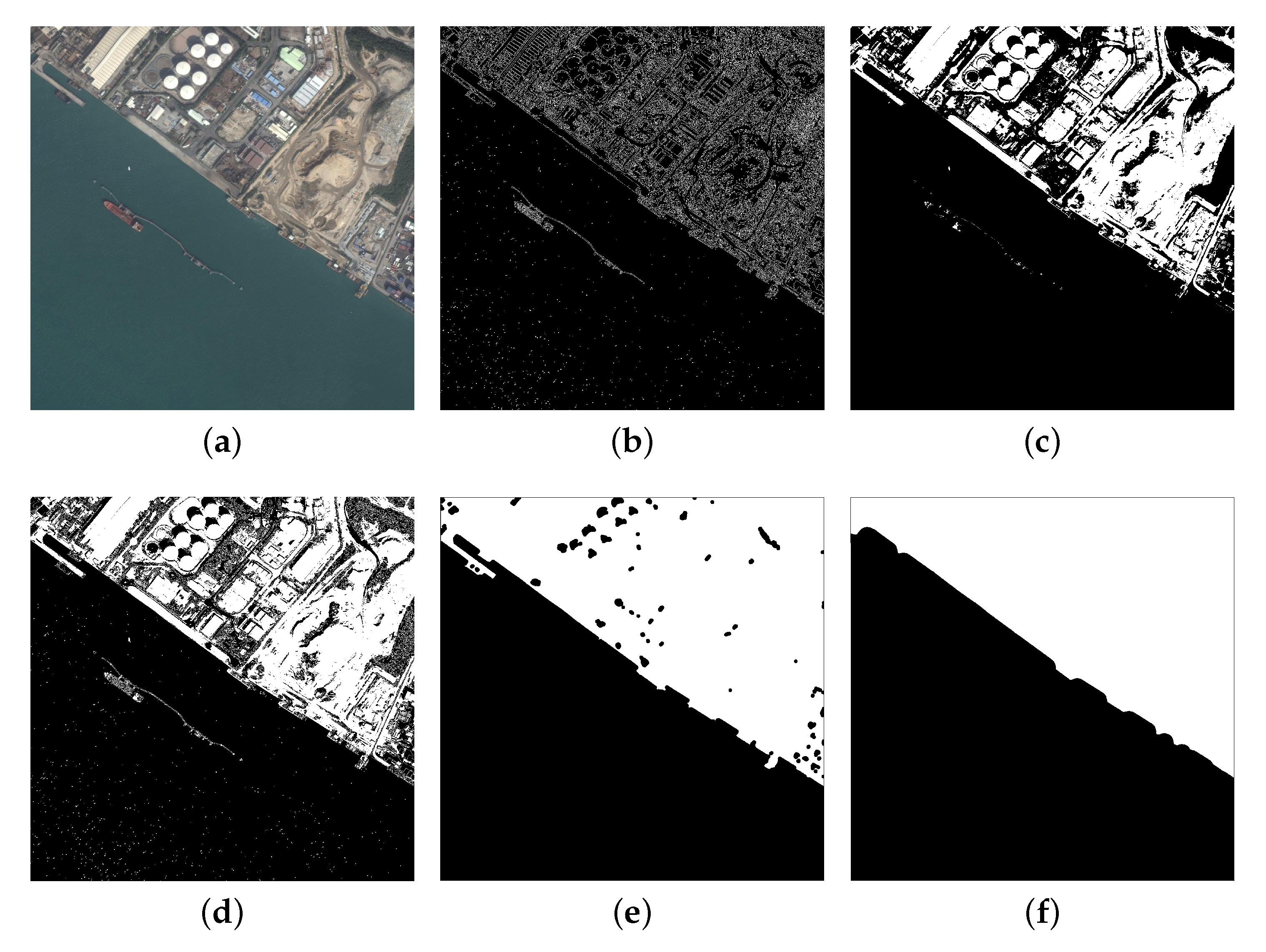
(3) Finally, a series of specific morphological operations are performed on this binary image. The basic specific morphological operation algorithms include dilation operation, erosion operation, open operation and close operation. Among them, the dilation operation and the close operation can fill gaps in the land contours of the binary map and remove small holes, while the erosion operations and the open operations can eliminate some small protrusions and narrow sections in the land area. Here, we first perform dilation operation and close operation on the binary image to eliminate the small holes in the land area. Then we calculate the connected regions for the processed binary image and exclude the small regions (corresponding to the ship or the small island at sea). The bumps on the land edges are eliminated by the erosion operation and the opening operation. The above specific morphological operation can be repeated to ensure the sea and land areas are completely separated. The size and shape of structuring elements is determined by analyzing the characteristic of non-connected areas on land from every experiment. The shape of structuring elements that selected in our experiment is disk, and the size of disk is 5 and 10. Figure 4 gives the intermediate results of a typical image slice in the sea-land separation process.
During test, only the area that contains the water area is sent into CF-SDN to detect ships and the pure land area is ignored.
Figure 4 gives the intermediate results of a typical image slice in the sea-land separation process. It can be found that the results of edge detection and threshold segmentation can complement each other to highlight non-water areas more completely. When only use threshold segmentation method, the area with low gray values on land may be classified as sea areas. Edge detection highlights the areas with complex textures and complements the results of threshold segmentation. We perform the expansion filtering and closing operations on the combined results in sequence. Then the connected regions are calculated and the small regions are removed. The final sea-land separation results highlight the land area and ships on the surface are classified as sea area.

2.2. Multi-Scale Detection Strategy

Generally the optical remote sensing images size is very large. The length and width of the image is usually several thousand pixels, the ship targets seem to be very small on the entire image. Therefore, it is necessary to cut the entire remote sensing image into some image slices and detect it separately. These image slices are normalized to the fixed size ( 320 × 320 ) in a certain proportion. Then the coarse-to-fine ship detection network outputs the detection results of these image slices. Here, the outputs of network are scaled according to the corresponding proportion. Finally, these detection results are mapped back to the original image according to the cutting position.
The sea-land separation results obtained in the previous subsection will also be applied in this subsection. Most ship detection methods set the pixel value of the land area in the remote sensing image to zero or the image’s mean value to achieve the purpose of shielding land during the detection process. However, roughly removing original pixel values of the land area can easily lead to miss detection of ships at boundary between sea and land. If separation results are not accurate enough, detection performance will be greatly reduced. In this paper, we use a threshold to quickly exclude the areas that only contain land, and detect ships in areas that contain water (include the boundary between the sea and land). The specific method is as follows:
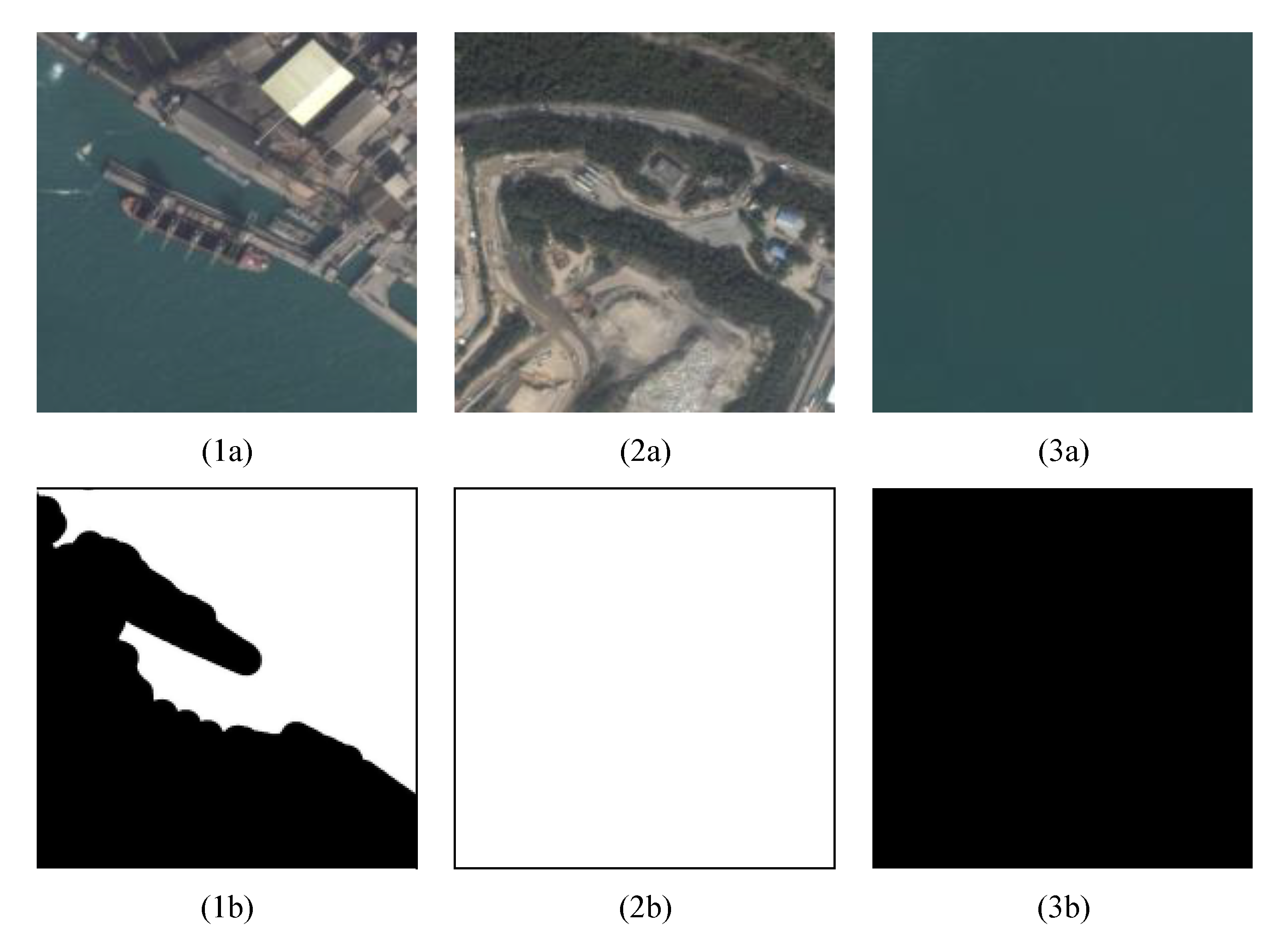
First, when the testing optical remote sensing image is cut, the corresponding sea-land separation result (a binary image) will be cut into some binary image slices with the same cutting method. And In the cut image, the ratio of ship area to slice area will become larger. Through a lot of experimental and statistical analysis, we found that when the average value of each binary image slice is less than a certain threshold, the water area in the image slice does not appear the ships. So each remote sensing image slice corresponds to a binary image slice. Figure 5 lists 3 examples. We calculate the average value of each binary image slice, and determine whether the image contains water. If the value is greater than the set threshold (0.8), we can think the corresponding remote sensing image slice almost does not contain water area, so we skip it and do not detect it.
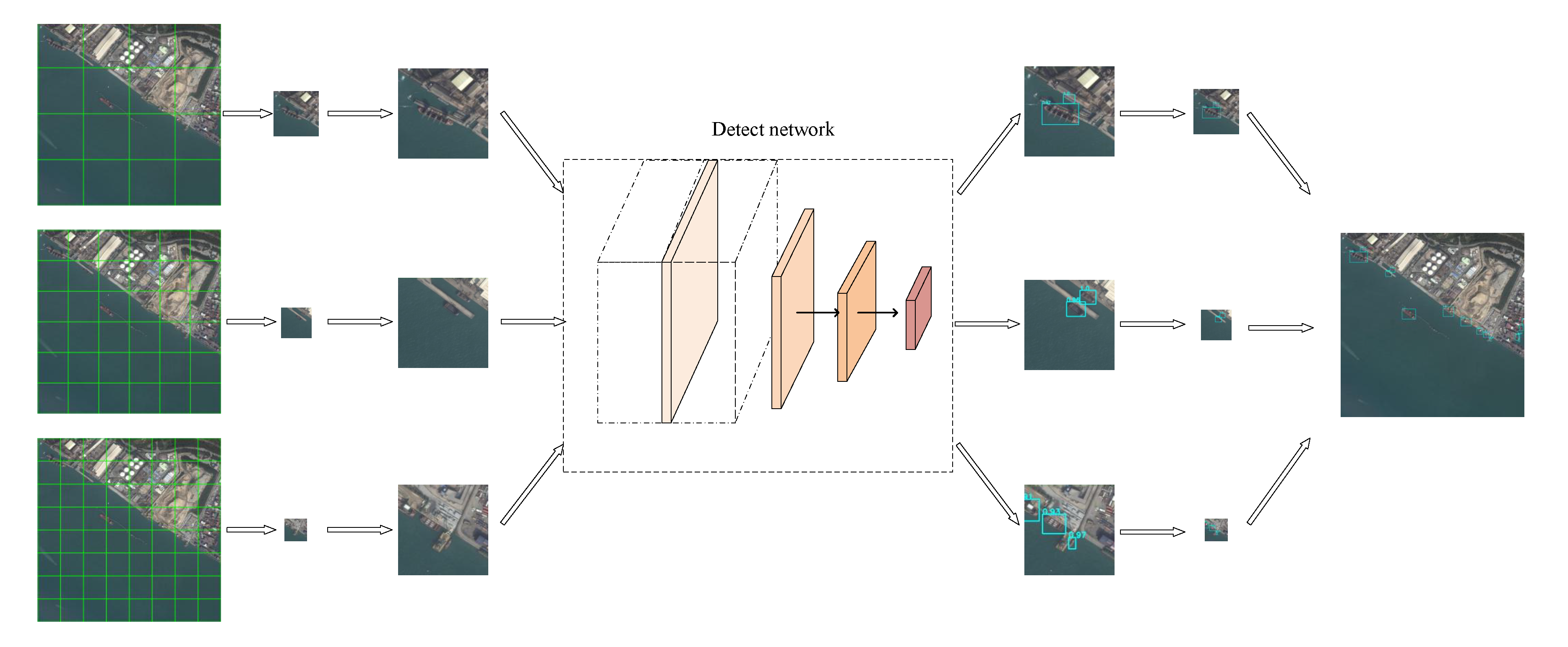
All mentioned above is the method using a single cutting size to cut and detect the testing optical remote sensing image. However, the scale distribution range of ships is wide. The size of small ship is only dozens of pixels, while the size of large ships is tens of thousands of pixels. It is difficult to determine the cutting size to ensure that ships at all scales can be accurately predicted. If the cutting size is small, many large ships will be cut off, which leads to miss detection. If the cutting size is large, many small ships will look smaller, which are difficult to detect. We propose a multi-scale detection strategy shown in Figure 6 to solve this dilemma.
The multi-scale detection strategy is that multiple cutting sizes are used to cut the testing optical remote sensing image into multiple different scales image slices in the test process. The testing optical remote sensing image is detected with multiple cutting sizes to achieve different degrees of refinement detection. And the detection results at each cutting size are combined to make the ship detection in optical remote sensing image more detailed and accurate.
In the experiment, we do a lot of tests and statistical analysis on the data set used in the experiments, and we find that the maximum length of the ship in the data does not exceed 200 pixels, the maximum width does not exceed 60 pixels, the minimum length is greater than 30 pixels, and the minimum width is greater than 10 pixels. Finally, the image slices can achieve satisfactory results when we choose the three cutting scales, 300 × 300 , 400 × 400 and 500 × 500 respectively. And then image slices of each scale are detected separately. The detection results at multiple cutting sizes are combined and most of the redundant bounding boxes are deleted by non-maximal suppression (NMS), then we obtain the final detection results.

2.3. Elimination of Cutting Effect

Because the optical remote sensing images need to be cut during the detection process, many ships are easy to be cut off. This results in some bounding boxes which are output by the network only containing a portion of the ship. We adopt two strategies to eliminate the effect of cutting.
(1) We slice the image by overlap cutting. The overlap cutting is a strategy to ensure each ship appears completely at least once in all cutting image slices. This strategy produces overlapping slices by moving stride smaller than the slice size. For example, when the slice size is 300*300, the stride must be less than 300, and the produced slices certainly have overlapping parts. Moreover, different cutting scales are used in the test process. The ship which is cut off at one scale may completely appear at another scale. These bounding boxes detected from each image slice are mapped back to the original image according to the cutting position, which ensure that at least one of the bounding boxes of the same ship can completely contain the ship. The overlap cutting size used in experiment is 100 and the stride is 100.
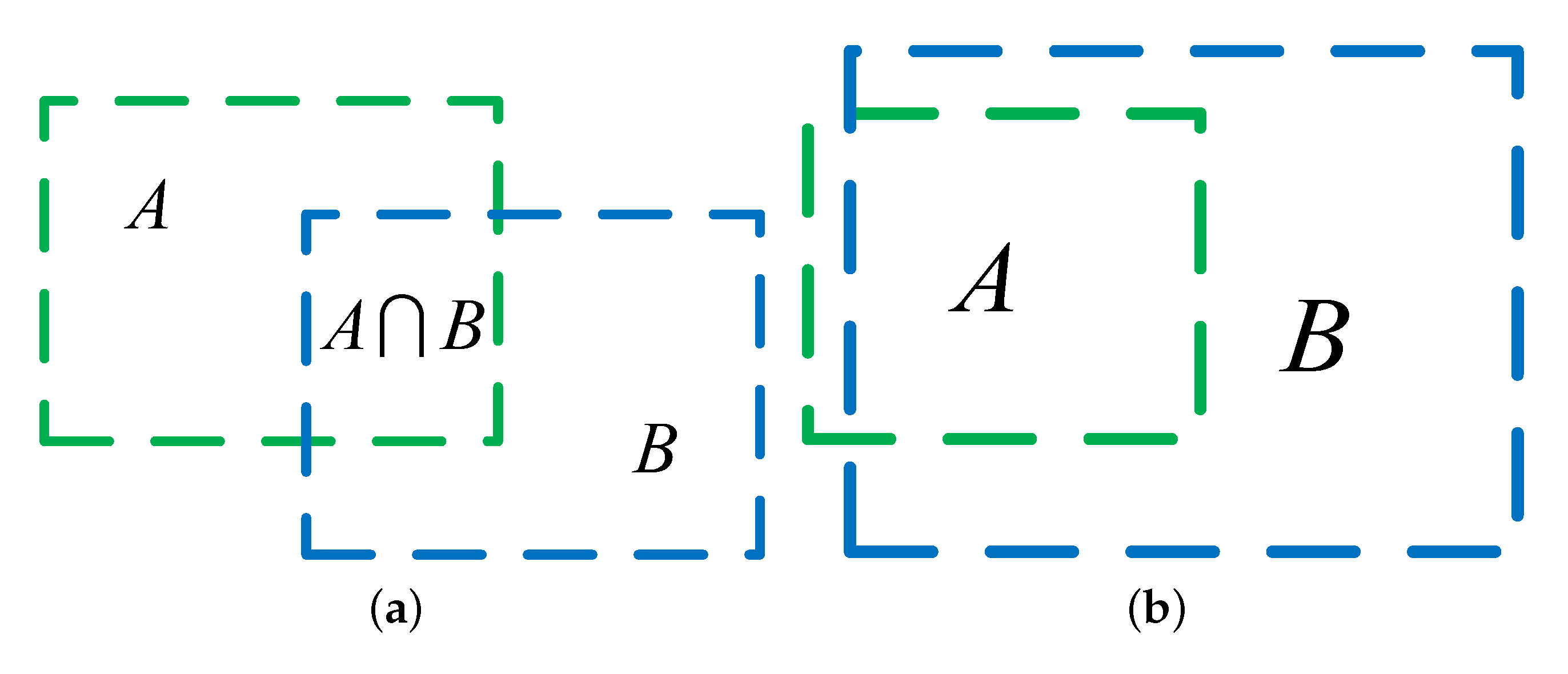
(2) Suppose there are two bounding boxes A and B, shown in Figure 7a. The original NMS method calculates the Intersection over Union (IoU) of the two bounding boxes and compares it with the threshold to decide whether to delete the bounding box with lower confidence. However, optical remote sensing image ship detection is special. As shown in Figure 7b, it is assumed that the bounding box A only contains a part of a ship, and the bounding box B completely contains the same ship, so most of the area A is contained in B. But according to the above calculation method, the IOU between A and B may not exceed the threshold, so the bounding box A is retained and becomes a redundant bounding box.
In order to solve this situation, a new metric named IOA (intersection over area) is used in the NMS to determine whether to delete the bounding box. We define IOA between box A and box B as:
I O A = a r e a ( A B ) a r e a ( B )
Here, assuming that the confidence of B is lower than A (if the confidence of the two boxes is equal, then box B is the smaller one.) and a r e a ( A B ) refers to the area of the overlap between box A and box B.
During the test, we first perform non-maximum suppression on all detection results, which calculates the value of IOU between overlapping bounding boxes (the threshold is 0.5) to remove some redundant bounding boxes. For the remaining bounding boxes, the IOA between the overlapping bounding boxes are calculated. If the IOA between the two bounding boxes exceeds the threshold which is set to 0.8 in the experiments, the bounding box with lower confidence is removed. The remaining bounding boxes are the final detection results.

2.4. The Feature Extraction Structure

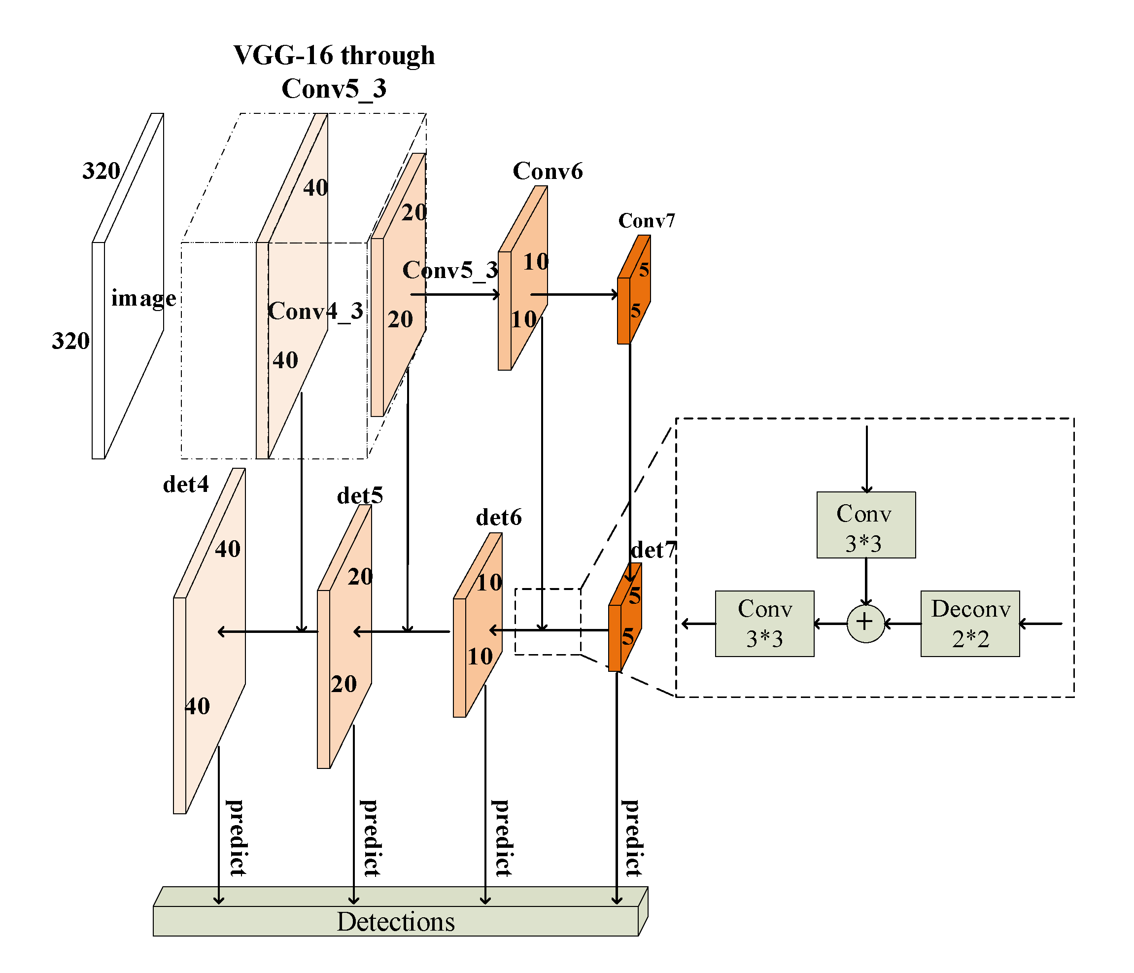
Using deep convolutional neural networks for target detection have an important problem. It is that the feature map output by the convolutional layer becomes smaller as the network deepens, and the information of the small target is also lost. This causes low detection accuracy for small target. Considering that shallow feature maps have higher resolution and deep feature maps contain more semantic information, we used FPN [43] to solve this problem. This structure can fuse features of different layers and independently predict object position of each feature layer. Therefore, the CF-SDN not only can preserve the information of small ship, but also have more semantic information. The input of the network is an image slice which is cut from optical remote sensing images, and the output is the predicted bounding boxes and the corresponding confidences. The feature extraction structure of the CF-SDN is shown in the Figure 8.
We select the first 13 convolutional layers and the first 4 max pooling layers of VGG-16 which is pre-trained with ImageNet dataset [44] as the basic network, and add 2 convolutional layers ( c o n v 6 and c o n v 7 ) at the end of the network. The two convolutional layers ( c o n v 6 and c o n v 7 ) reduce the resolution of the feature map to half in sequence. With the deepening of the network, the features are continuously sampled by the max pooling layer, and the resolution of the output feature map get smaller, but the semantic information is more abundant. This is similar to the bottom-up process in FPN networks(A deep convnet computes an inherent multi-scale and pyramidal shape feature hierarchy). We select four different resolution feature maps that output from c o n v 4 _ 3 , c o n v 5 _ 3 , c o n v 6 and c o n v 7 , as shown in Figure 8. The strides of the selected feature maps are 8, 16, 32 and 64. The input size of this network is 320 × 320 pixels and the resolutions of the selected feature map are 40 × 40 ( c o n v 4 _ 3 ), 20 × 20 ( c o n v 5 _ 3 ), 10 × 10 ( c o n v 6 ) and 5 × 5 ( c o n v 7 ).
We set four detection layers in the network, and generate four feature maps of corresponding size through the selected feature maps. Then these feature maps are used as the input of four detection layers respectively. The deepest feature map ( 5 × 5 ) output by c o n v 7 is directly considered as the feature map of the last detection layer input, which is named det7. The feature maps used as inputs of the remaining detection layers are generated sequentially from the back to front in a lateral connections manner. The dotted line in the Figure 8 demonstrates the lateral connections manner. The deconvolution layer doubles the resolution of the deep feature map, while the convolution layer only changes the channel number of the feature map without changing the resolution. Feature maps are fused by element addition, and a 3 × 3 convolutional layer is added to decrease the aliasing effect caused by up-sampling. The fusion feature map serves as the input of the detection layer.

2.5. The Distribution of Anchors

In this subsection, we design the distribution of anchors at each detection layer. Anchors [28] are a set of reference boxes at each feature map cell, which tile the feature map in a convolutional manner. At each feature map cell, we predict the offsets relative to the anchor shapes in the cell and the confidence that indicate the presence of ship in each of those boxes. In optical remote sensing images, the scale distribution of ships is discrete, and ships usually have diverse aspect ratio depending on different orientations. So anchors with multiple sizes and aspect ratios are set at each detection layer to increase the number of matched anchors.
Feature maps from different detection layer have different resolutions and receptive field sizes introduce two types of receptive fields in CNN [45,46], one is the theoretical receptive field which indicates the input region that theoretically affects the value of this unit, the other is the effective receptive field which indicates the input region has effective influence on the output value. Zhang et al. [47] points out that the effective receptive field is smaller than the theoretical receptive field, and anchors should be significantly smaller than theoretical receptive field in order to match the effective receptive field. At the same time, the article states that the stride size of a detection layer determines the interval of its anchor on the input image.
As listed in the second and third column of Table 1, the stride size and the size of theoretical receptive field at each detection layer are fixed. Considering that the anchor size set for each layer should be smaller than the calculated theoretical receptive field, we design the anchor size of each detection layer as shown in the fourth column of Table 1. The anchors of each detect layer have two scales and five aspect ratios. The aspect ratios are set to { 1 3 , 1 2 , 1 , 2 , 3 } , so there are 2 × 5 = 10 anchors at each feature map cell on each detection layer.

2.6. The Coarse-to-Fine Detection Strategy

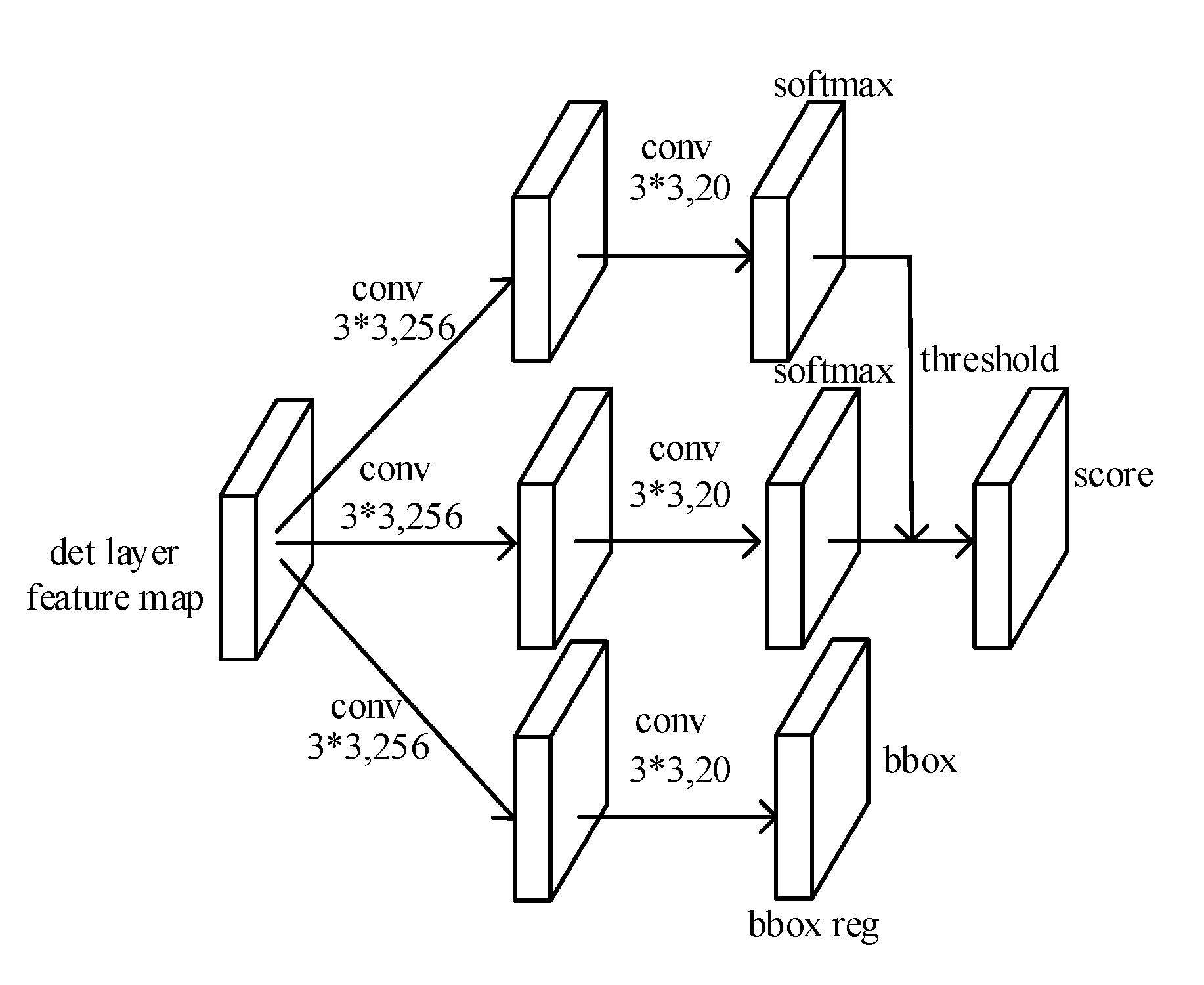
The structure of the detection layer is shown in Figure 9. We set up three parallel branches at each detection layer, two for classification and the other for bounding box regression. In Figure 9, the branches from top to bottom are coarse classification network, fine classification network and bounding box regression network, respectively. At each feature map cell, the bounding box regression network predicts the offsets relative to the anchor shapes in the cell, and the coarse classification network predicts the confidence which indicates the presence of ship in each of those boxes. This is a coarse detection process which obtains some bounding boxes with confidences. Then, the image block contained in the bounding box which has a confidence higher than the threshold (set to 0.1) is further classified (ship or background) by the fine classification network to obtain the final detection result. This is a fine detection process.

2.6.1. Loss Function

Aiming at the structure of the detection layer, the multi-task loss L are used to jointly optimize model parameters:
L = α 1 N c l s 1 i L c l s ( p i , p i * ) + β 1 N r e g i p i * L r e g ( t i , t i * ) + γ 1 N c l s 2 j L c l s ( p j , p j * )
In Equation (2) i is the index of an anchor from the coarse classification network and the bounding box regression network in a batch, and p i is the predicted probability that the anchor i is a ship. If the anchor is positive, the ground truth label p i * is 1, and p i * is 0 conversely. t i is a vector representing the 4 parameterized coordinates of the predicted bounding box, and t i * is that of the ground-truth box associated with a positive anchor. The term p i * L r e g means the regression loss is activated only for positive anchors and disabled otherwise. j is the index of an anchor from the fine classification network in a mini-batch, and the meaning of p j and p j * is similar to p i and p i * . The three terms are normalized by N c l s 1 , N r e g and N c l s 2 and weighted by the balancing parameter α , β and γ . N c l s 1 represents the number of positive and negative anchors from the coarse classification network in the batch. N r e g represents the number of positive anchors from the bounding box regression network in the batch, and N c l s 2 represents the number of positive and negative anchors from the fine classification network in the batch. In our experiment, we set α = β = γ = 1 3 .
In Equation (2) the classification loss L c l s is the log loss from the coarse classification network:
L c l s ( p i , p i * ) = - l o g [ p i * p i + ( 1 - p i ) ( 1 - p i * ) ]
the regression loss L r e g is the smooth L1 loss from the bounding box regression network:
L r e g ( t i , t i * ) = R ( t i - t i * )
R is smooth L1 function:
s m o o t h L 1 ( x ) = 0 . 5 x 2 i f x < 1 , x - 0 . 5 o t h e r w i s e

2.6.2. Training Phase

In the training phase, these three branches are trained at the same time. A binary class label is set for each anchor in each branch.
(1) For coarse classification network and bounding box regression network, the anchors assigned positive label must satisfy one of the following two conditions: (i) match a ground truth box with the highest Intersection-over-Union (IoU) overlap. (ii) match a ground-truth box with an IoU overlap higher than 0.5. The anchors which have IoU overlap lower than 0.3 for all ground-truth boxes are assigned as negative label. The SoftMax layer outputs the confidences of each anchor at each cell on the feature map. Anchors whose confidence higher than 0.1 are selected as the train samples of the fine classification network.
(2) For fine classification network, the anchors selected from the previous step are further given positive and negative label. Here, the IoU overlap threshold for selecting the positive anchor is raised from 0.5 to 0.6. The larger threshold means that the positive anchor selected is closer to the ground truth box, which makes the classification more precise. Since the number of negative samples in remote sensing images is much larger than the number of positive samples, we randomly select negative samples to ensure that the ratio between positive and negative samples in each mini-batch is 1:3. If the number of positive samples is 0, the number of negative samples is set to 256.

2.6.3. Testing Phase

In the testing phase, firstly the bounding box regression network outputs the coordinate offsets to each anchor at each feature map cell. Then we adjust the position of each anchor by the box regression strategy and to get the bounding boxes. The outputs of the two classification networks are the confidence scores s1 and s2 corresponding to each bounding box. The confidence scores encode the probability of the ship appearing in the bounding box. First, if s1 output from the coarse classification network is lower than 0.1, the corresponding bounding box is removed. Then the confidence corresponding to the remaining bounding box is determined as the product of s1 and s2. The bounding box with the confidence larger than 0.2 is selected. Finally, non-maximum suppression (NMS) is applied to get final detection results.

3. Experiments and Results

In this section, the details of the experiments are described and the performances of the proposed method are studied. First, we introduce the data set used in the experiment. Then we introduce evaluation metrics used in the experiments. Finally, we conduct multiple sets of experiments to evaluate the performance of our methods and compare it with three excellent detection methods.

3.1. Data Set

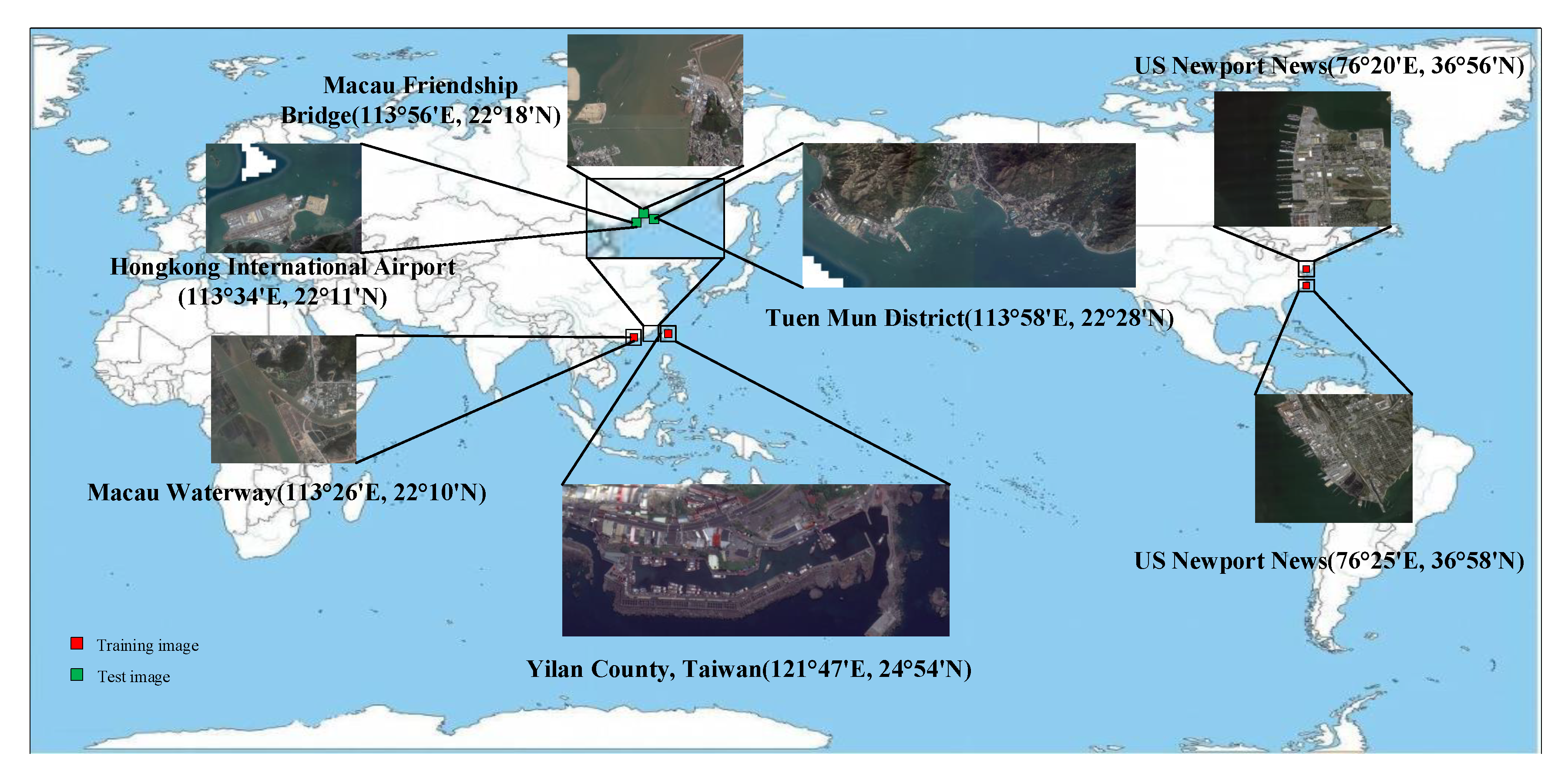
Due to the lack of public data sets intended for ship detection in optical remote sensing image, we collected seven typical and representative images from different geographic conditions in Google Earth. The resolution of these images is 0.5 meter per pixel. The number of ships contained in each image range from dozens to hundreds and the ship size varies from 10 × 10 pixels to 400 × 400 pixels. Among these images, we selected 4 images for training and 3 images were remained for testing. The position of each ship in training images were labeled, including the coordinates of the center point, length and width of the ship. The data set we used is shown in Figure 10. Table 2 introduces the three images IMAGE1, IMAGE2, and IMAGE3 of the testing set.
For training set images, the center of each ship was regarded as the center of image slice and some image slices were cut out as the train samples with the size of 300 × 300 , 400 × 400 , and 500 × 500 . Data augmentation was achieved through translation, rotation, image brightness, contrast changes and so on. After data augmentation, 30000 image slices with different sizes composed the training data set for CF-SDN. Each ship is completely contained in at least an image slice and the corresponding position information constituted the training label set.

3.2. Evaluations Metrics

The precision-recall curve (PRC) and average precision (AP) are used to quantitatively evaluate the performance of an object detection system.

3.2.1. Precision-Recall Curve

The precision-recall curve reflects the trend in precision and recall. The precision rate represents the proportion of the real target in the predicted target, and the recall rate represents the proportion of the correctly detected targets in the actual real targets. The precision and recall metrics are computed as follows:
p r e c i s i o n = N t p N t p + N f p
r e c a l l = N t p N t p + N f n
Here, N t p represents the number of true positives, which indicates the number of the correctly detected targets. N f p represents the number of false positives, which indicates the number of the error detected targets(misjudge the background as a target). N f n represents the number of false negatives, which indicates the number of miss detected targets. If the IoU between the predicted bounding box and the ground truth bounding box exceeds 0.5, the detection is regarded as true positive, otherwise, as a false positive. If there are multiple predicted bounding boxes overlap the same ground truth bounding box, then only one is considered as true positive, while others are considered as false positive.
The higher precision rate and recall rate, the better detection performance. But the precision rate is usually balanced against the recall rate. When the recall rate increases, the precision rate will decrease accordingly. Therefore, we calculate the average precision of the P-R curve to reflect the detection performance.

3.2.2. Average Precision

The average precision is the area under the precision-recall curve. Here, the average precision is obtained by calculating the average value of the corresponding precision when the recall rate changes from 0 to 1. In this paper, the average precision is calculated by the method used in the PASCAL VOC Challenge, which calculates the average precision by taking the mean of the precision rate of the points at all different recall rates on the P-R curve.

3.3. Implementation Details

Our experiments are implemented in Caffe, in a hardware environment consisting of HP-Z840 Workstation with an TITAN X12-GB GPU.
In the training of CF-SDN, the layers from VGG-16 are initialized by pre-training a model for ImageNet classification [48], which is a common technique used in deep neural networks. All other new layers are initialized by drawing weights from a zero-mean Gaussian distribution with standard deviation 0.01. The whole network is trained end-to-end by back propagation algorithm and SGD. The initial learning rate is set to 0.001 and we use it for 30k iterations; then we continue training for 30k iterations with 0.0005. The batch size is set to 20, and the total number of positive anchors and negative anchors in a batch is 256. The momentum is set to 0.9 and the weight decay is set to 0.0005.

3.4. Experimental Results and Analysis

3.4.1. Performance on the Testing Data Set

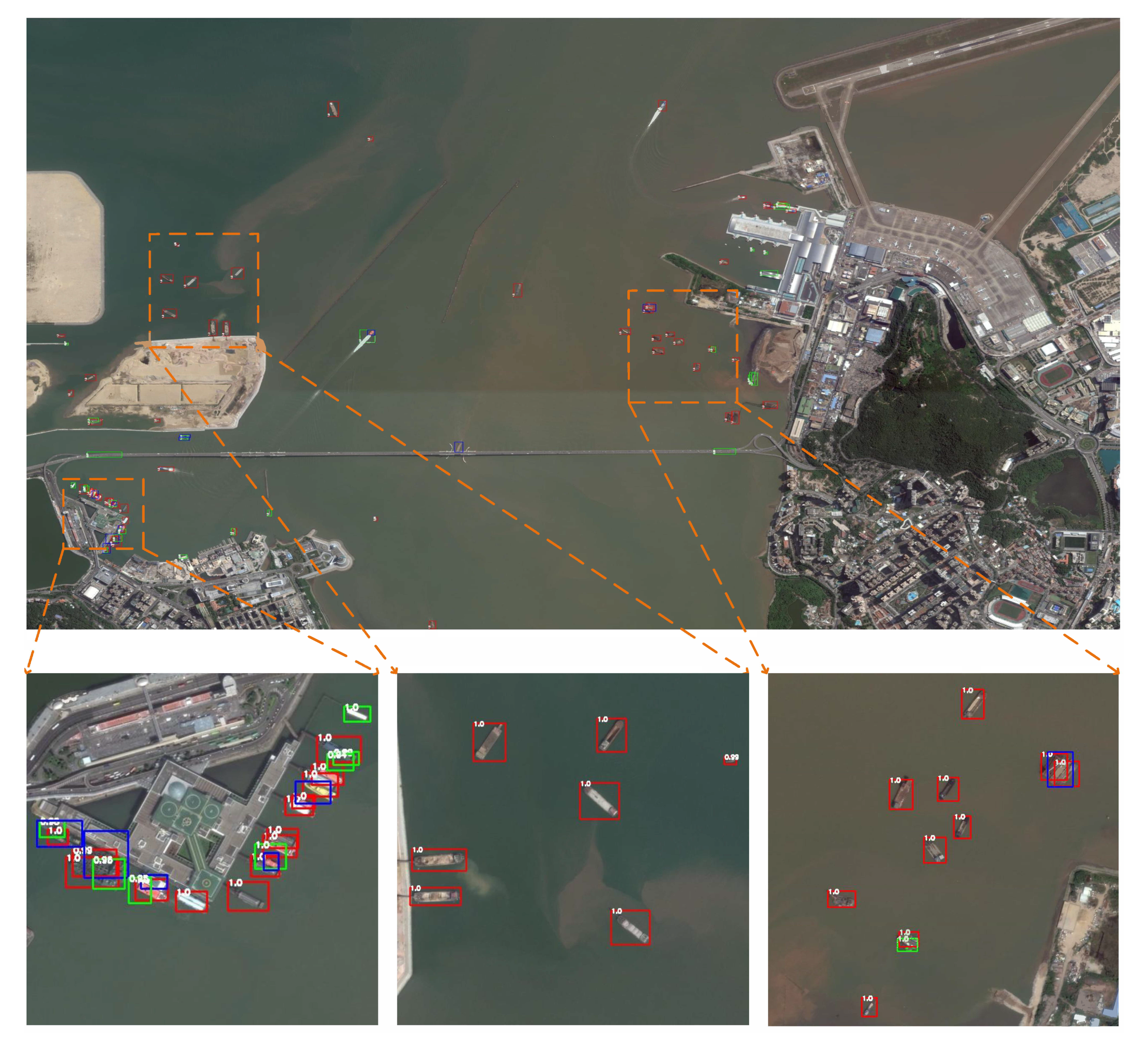
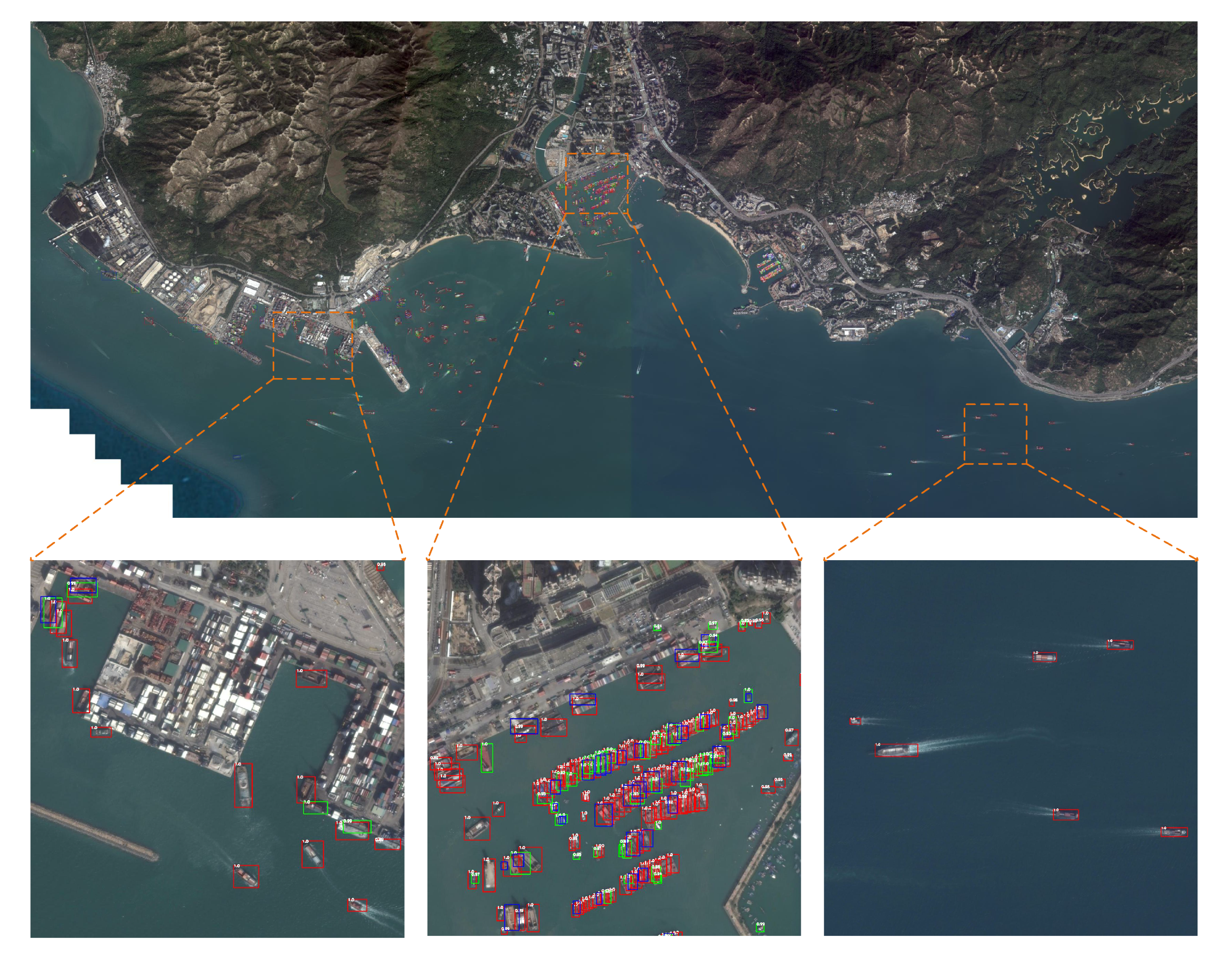
Using the trained CF-SDN, we perform ship detection on the testing data set which contains three optical remote sensing images with different scenes. The sea-land separation algorithm is used to obtain a binary image of the testing image, which is used to remove the image slices that only contain land. The multi-scale detection strategy is used to achieve different degrees of refinement detection. Figure 11, Figure 12 and Figure 13 shows the detection results of CF-SDN on IMAGE1, IMAGE2 and IMAGE3 respectively, in which the true positives, false positives and false negatives are indicated by red, green and blue rectangles. The top left corner of the rectangle shows the confidence. Due to the large size of the testing image, we only take some representative areas to show the details.
As shown in Figure 11, the proposed method exhibits good detection performance for small size ships. Despite some ships on the sea are fuzzy which caused by cloud occlusion and wave interference, the proposed method has successfully detected most of these ships. As shown in Figure 12 and Figure 13, the proposed method has accurately located the scattered ships on the sea. Many ships on the land boundary also can be well detected, though they are easily be confused with the land features. For the dense ships in the port, as shown in Figure 13, our method can also detect most of the ships.

3.4.2. Comparison with other detection algorithms

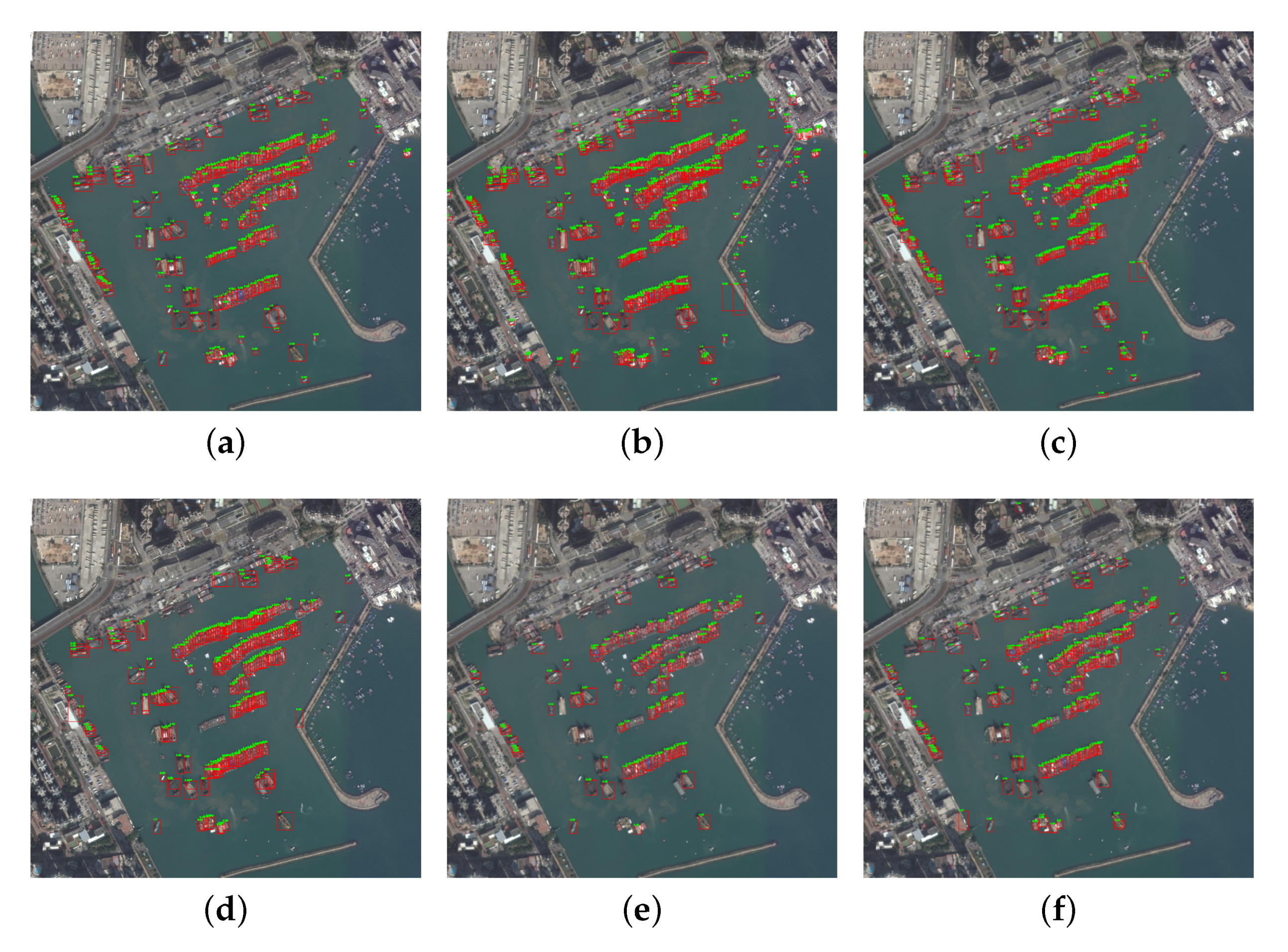
In order to quantitatively demonstrate the superiority of our approach, we compared it with the other object detection algorithms. We choose R-CNN [33], Faster R-CNN [28], SSD [37] and the latest ship detection algorithms [49] as the comparison algorithm. R-CNN is an object detection model based on deep convolutional neural network and has been widely used in object detection of remote sensing images. Faster R-CNN is the representative two-stage object detection model and is improved from R-CNN. SSD is the representative one-stage object detection model, which is the same as CF-SDN and achieves an end-to-end mapping directly from image pixels to bounding box coordinates. The latest ship detection algorithm is a R-CNN based ship detection algorithm. Figure 14 is shown the specific example from six different methods.
In addition, to further validate the effectiveness of the proposed feature extraction structure and the coarse-to-fine detection strategy, we compare the proposed CF-SDN with CF-SDN without fine classification. In this experiment, C-SDN represents the CF-SDN without fine classification network, which has the same feature extraction structure as CF-SDN, but only contains a coarse classification network and a bounding box regression network at the detection layer. CF-SDN represents the complete CF-SDN, which adopts the coarse-to-fine detection strategy in detection, and predicts the boundary box that may contain ships through a coarse classification network and a bounding box regression network, and further finely classifies the detection results through a fine classification network.
For all test methods, the sea-land separation algorithm was implemented to remove the image slice that only contains land. We used the overlap cutting to slice the images the cutting size used in test is 400 (the overlap cutting size is 100 and the stride is 100). In addition, the detection results of the whole testing images are processed by NMS, and the IOA threshold is set to 0.5.
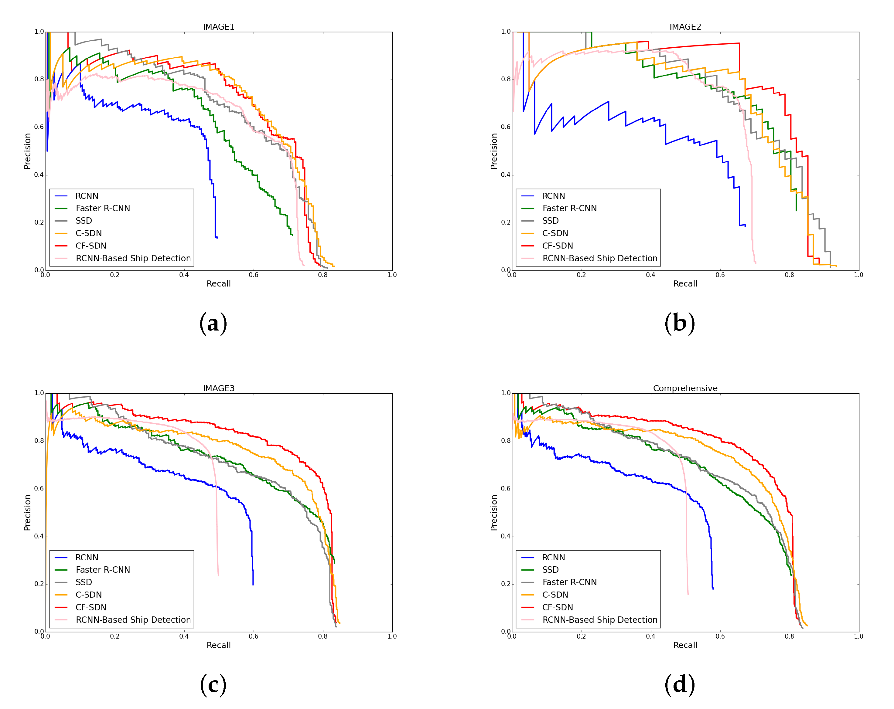
Table 3 and Table 4 and Figure 15 show the quantitative comparison results of these methods on testing data set. As can be seen, the proposed CF-SDN exceed all other methods for all images in terms of AP. Compared with R-CNN, SSD, Faster R-CNN, C-SDN and R-CNN Based Ship Detection, the proposed CF-SDN acquires 27.3%, 9.2%, 4.8%, 2.7%, 22.4% performance gains in terms of AP on entire data set, respectively. Among them, the performance of C-SDN is second only to CF-SDN. Compared with R-CNN, SSD, Faster R-CNN and R-CNN Based Ship Detection, the CF-SDN without fine classification (C-SDN) acquires 24.6%, 6.5%, 2.1%, 21.7% performance gains in terms of AP on entire data set, respectively. This benefits from the proposed feature extraction structure which fuses different hierarchical features to improve the representation of features. Through the comparion between the C-SDN and CF-SDN, we can find the superiority of the coarse-to-fine detection strategy. Many false alarms are removed and the average precision is improved by the further fine classification.

3.4.3. Sea-Land Separation to Improve the Detection Accuracy

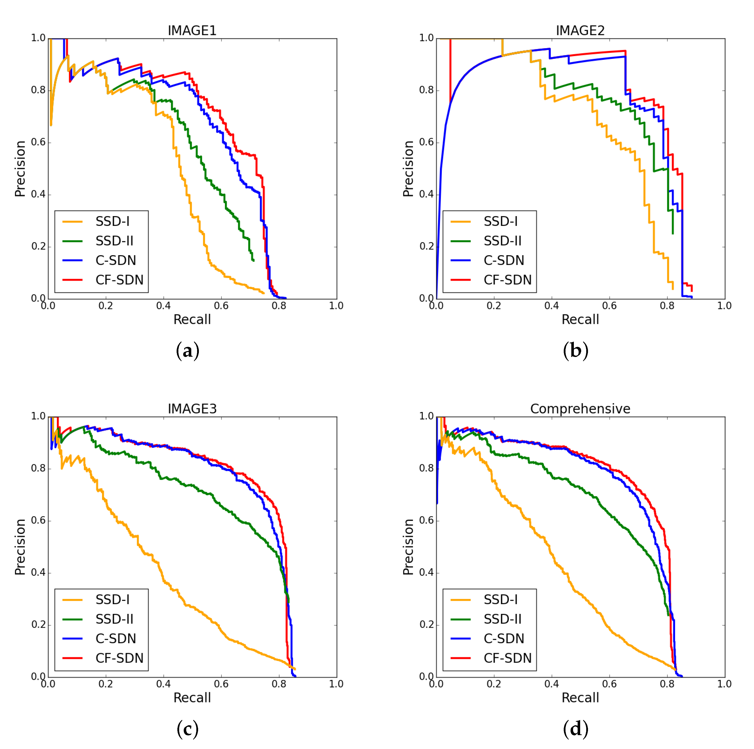
In order to validate the effectiveness of the sea-land separation algorithm, we compared the detection results with and without sea-land separation during the test. We choose SSD and CF-SDN as the detection model. SSD-I and C-SDN indicate that the sea-land separation method was not used during the test. SSD-II and CF-SDN indicate that the proposed sea-land separation method is used to remove the areas which only contain land during the test. The cutting size is 400 (the overlap is 100). The detection result of the whole testing image is processed by NMS, and the IoU threshold is set to 0.5.
Table 5 shows the quantitative comparison results of the experiments. Table 6 shows the time spent in two different phases during the test. It can be observed that SSD-II acquires 19.6% performance gains in terms of AP in entire data set compared with SSD-I, while CF-SDN acquires 2.1% performance gains compared with C-SDN. As shown in Figure 16, the method that use sea-land separation has achieved higher accuracy when the recall rate is almost equal. This demonstrates that the sea-land separation can avoid some false alarms and improve the detection accuracy. The detection performance of SSD is more affected by sea-land separation than that of CF-SDN, which confirms that CF-SDN can extract features better and generate fewer false alarms.

3.4.4. Multi-Scale Detection Strategy Improves Performance

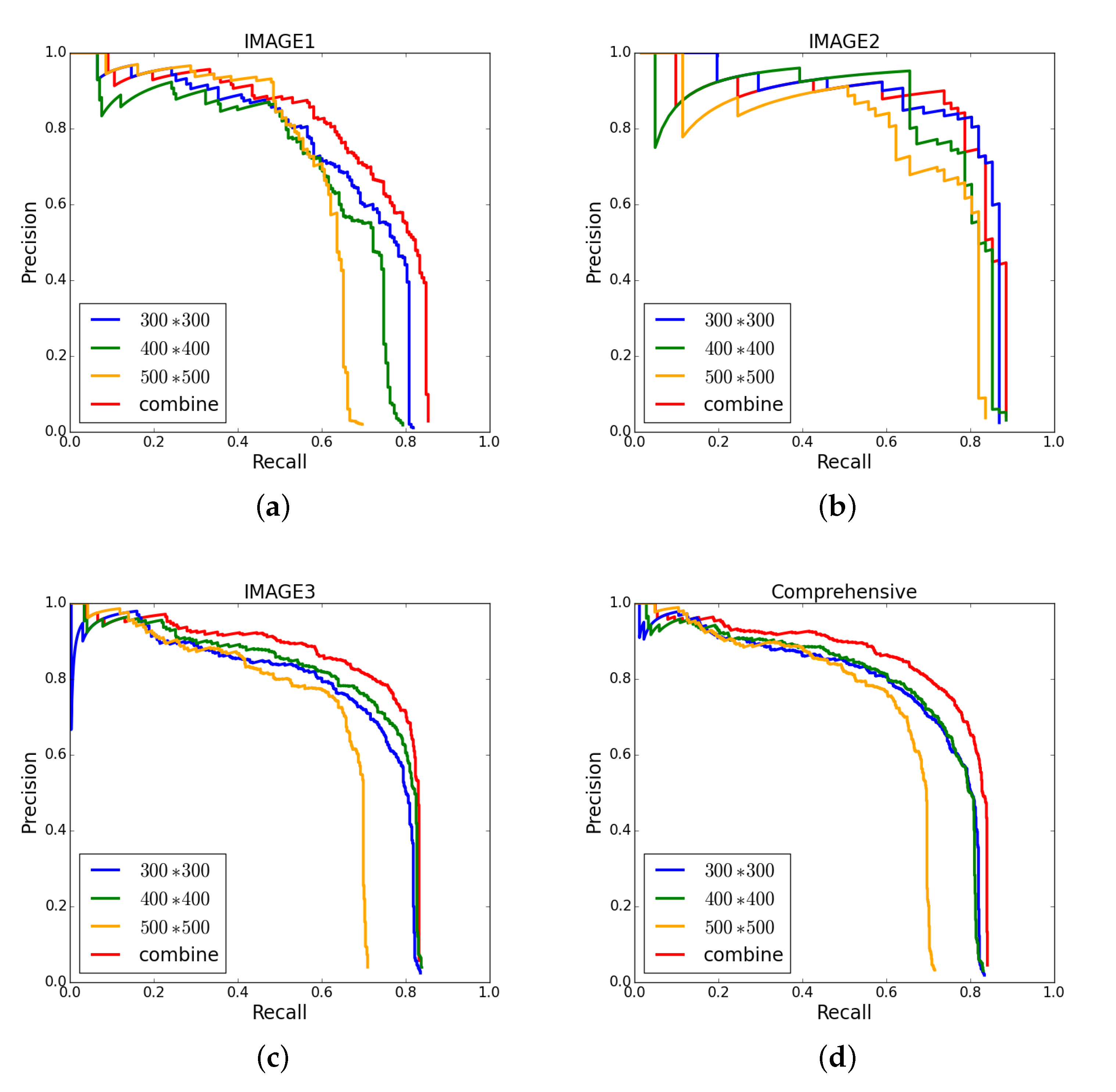
In order to validate the effectiveness of the multi-scale detection strategy, we compare the detection performance of using single cutting size and using multi-scale detection strategy during the test. For the experiment that using single cutting size, we adopt three different cutting sizes of 300 × 300 , 400 × 400 and 500 × 500 respectively. For the experiment that using multi-scale detection strategy, we combine the detection results of three single cutting size and use NMS to remove some redundant bounding boxes. The detection model used in these experiments is the CF-SDN, and both of them use the sea-land separation algorithm to remove the area that only contains land.
Table 7 and Figure 17 show the quantitative comparison results of using each single cutting sizes and using the multi-scale detection strategy. As can be seen from them, the highest detection accuracy is obtained by using the multi-scale detection strategy. When we only adopt a single cutting size, the cutting scale of 400 × 400 demonstrates the best detection performance on the testing data set. Compared with the single detection scale of 300, 400, 500, the combined result acquired 4.4%, 3.9%, 13.8% performance gains in terms of AP in entire data set. Combined with the detection results at different cutting sizes, the multi-scale detection strategy shows the outstanding advantages. The combination of multiple detection with different refinement degree effectively improves the accuracy and the recall of ship detection.

4. Conclusions

This paper presents a coarse-to-fine ship detection network (CF-SDN) which includes a sea-land separation algorithm, a coarse-to-fine ship detection network and a multi-scale detection strategy. The sea-land separation algorithm can avoid false alarms on land. The coarse-to-fine ship detection network do not need to use the region proposal algorithm and directly achieves an end-to-end mapping directly from image pixels to bounding boxes with confidences. The multi-scale detection strategy can achieve ship detection with different degrees of refinement. It effectively improves the accuracy and speed of ship detection.
Experimental results on optical remote sensing data set show that the proposed method outperforms other excellent detection algorithms and achieves good detection performance on the data set including some small-sized ships. For the dense ships near the port, our method can locate most of the ships well, although produce a little false alarms and miss detections at the same time. The main reason for the missing detection is that many bounding boxes with high overlap are removed by NMS. In fact, the overlaps between the ground truth of dense ships is very high. Therefore, our future work will focus on the two aspects: (1) The orientation angle information is taken into account when determining the position of the ship, which can effectively reduce the overlap between the bounding boxes of the dense ships. (2) Combined with the characteristics of remote sensing images, the select strategy of positive and negative samples are considered in the network to improve the classification and location ability of the detection network.

Author Contributions

Y.W. and W.Z. conceived and designed the experiments; X.C. and Z.B. performed the experiments; Q.G. and X.C. analyzed the data; W.M., M.G. and Q.M. contributed materials; Z.B. wrote the paper. Y.W. and W.M. supervised the study and reviewed this paper. All authors have read and agreed to the published version of the manuscript.

Funding

This work was supported in part by National Natural Science Foundation of China (No. 61702392).

Acknowledgments

The authors would like to thank the anonymous reviewers for their very competent comments and helpful suggestions.

Conflicts of Interest

The authors declare no conflict of interest.

References

  1. Zhu, C.; Zhou, H.; Wang, R.; Guo, J. A Novel Hierarchical Method of Ship Detection from Spaceborne Optical Image Based on Shape and Texture Features. IEEE Trans. Geosci. Remote Sens. 2010, 48, 3446–3456. [Google Scholar] [CrossRef]
  2. Lang, F.; Yang, J.; Yan, S.; Qin, F. Superpixel Segmentation of Polarimetric Synthetic Aperture Radar (SAR) Images Based on Generalized Mean Shift. Remote Sens. 2018, 10, 1592. [Google Scholar] [CrossRef] [Green Version]
  3. Ciecholewski, M. River Channel Segmentation in Polarimetric SAR Images: Watershed Transform Combined with Average Contrast Maximisation. Expert Syst. Appl. 2017, 82, 196–215. [Google Scholar] [CrossRef]
  4. Braga, A.M.; Marques, R.C.; Rodrigues, F.A.; Medeiros, F.N. A Median Regularized Level Set for Hierarchical Segmentation of SAR Images. IEEE Geosci. Remote Sens. Lett. 2017, 14, 1171–1175. [Google Scholar] [CrossRef]
  5. Jin, R.; Yin, J.; Zhou, W.; Yang, J. Level Set Segmentation Algorithm for High-resolution Polarimetric SAR Images Based on a Heterogeneous Clutter Model. IEEE J. Sel. Top. Appl. Earth Obs. Remote Sens. 2017, 10, 4565–4579. [Google Scholar] [CrossRef]
  6. Schwegmann, C.P.; Kleynhans, W.; Salmon, B.P.; Mdakane, L.W.; Meyer, R.G. Very deep learning for ship discrimination in synthetic aperture radar imagery. In Proceedings of the 2016 IEEE International Geoscience and remote-sensing Symposium (IGARSS), Beijing, China, 10–15 July 2016; Volume 10, pp. 104–107. [Google Scholar]
  7. Bentes, C.; Frost, A.; Velotto, D.; Tings, B. Ship-iceberg Discrimination with Convolutional Neural Networks in High Resolution SAR Images. In Proceedings of the 11th European Conference on Synthetic Aperture Radar, Hamburg, Germany, 6–9 June 2016; Volume 6, pp. 1–4. [Google Scholar]
  8. Zhao, B.; Zhong, Y.; Zhang, L. A Spectral–structural Bag-of-features Scene Classifier for Very High Spatial Resolution remote-sensing Imagery. ISPRS J. Photogramm. Remote Sens. 2016, 116, 73–85. [Google Scholar] [CrossRef]
  9. Yang, G.; Li, B.; Ji, S.; Gao, F.; Xu, Q. Ship Detection from Optical Satellite Images Based on Sea Surface Analysis. IEEE Geosci. Remote Sens. Lett. 2013, 11, 641–645. [Google Scholar] [CrossRef]
  10. Bi, F.; Zhu, B.; Gao, L.; Bian, M. A Visual Search Inspired Computational Model for Ship Detection in Optical Satellite Images. IEEE Geosci. Remote Sens. Lett. 2012, 9, 749–753. [Google Scholar]
  11. Corbane, C.; Najman, L.; Pecoul, E.; Demagistri, L.; Petit, M. A Complete Processing Chain for Ship Detection Using Optical Satellite Imagery. Int. J. Remote Sens. 2010, 31, 5837–5854. [Google Scholar] [CrossRef]
  12. Soofbaf, S.; Sahebi, M.; Mojaradi, B. A Sliding Window-based Joint Sparse Representation (SWJSR) Method for Hyperspectral Anomaly Detection. Remote Sens. 2018, 10, 434. [Google Scholar] [CrossRef] [Green Version]
  13. Qi, S.; Ma, J.; Lin, J.; Li, Y.; Tian, J. Unsupervised Ship Detection Based on Saliency and S-HOG Descriptor from Optical Satellite Images. IEEE Geosci. Remote Sens. Lett. 2015, 12, 1451–1455. [Google Scholar]
  14. Ding, Z.; Yu, Y.; Wang, B.; Zhang, L. An Approach for Visual Attention Based on Biquaternion and Its Application for Ship Detection in Multispectral Imagery. Neurocomputing 2012, 76, 9–17. [Google Scholar] [CrossRef]
  15. Yang, F.; Xu, Q.; Li, B. Ship Detection from Optical Satellite Images Based on Saliency Segmentation and Structure-LBP Feature. IEEE Geosci. Remote Sens. Lett. 2017, 14, 602–606. [Google Scholar] [CrossRef]
  16. Uijlings, J.R.; Van De Sande, K.E.; Gevers, T.; Smeulders, A.W. Selective Search for Object Recognition. Int. J. Comput. Vis. 2013, 104, 154–171. [Google Scholar] [CrossRef] [Green Version]
  17. Miyamoto, H.; Uehara, K.; Murakawa, M.; Sakanashi, H.; Nasato, H.; Kouyama, T.; Nakamura, R. Object Detection in Satellite Imagery Using 2-Step Convolutional Neural Networks. In Proceedings of the IEEE International Geoscience and remote-sensing Symposium, Valencia, Spain, 22–27 July 2018; pp. 1268–1271. [Google Scholar]
  18. Chang, H.H.; Wu, G.L.; Chiang, M.H. Remote-sensing Image Registration Based on Modified SIFT and Feature Slope Grouping. IEEE Geosci. Remote Sens. Lett. 2019, 16, 1363–1367. [Google Scholar] [CrossRef]
  19. Dong, C.; Liu, J.; Xu, F.; Liu, C. Ship Detection from Optical remote-sensing Images Using Multi-Scale Analysis and Fourier HOG Descriptor. Remote Sens. 2019, 11, 1529. [Google Scholar] [CrossRef] [Green Version]
  20. Li, Z.; Yang, D.; Chen, Z. Multi-layer Sparse Coding Based Ship Detection for remote-sensing Images. In Proceedings of the IEEE International Conference on Information Reuse and Integration, San Francisco, CA, USA, 13–15 August 2015; pp. 122–125. [Google Scholar]
  21. Haigang, S.; Zhina, S. A Novel Ship Detection Method for Large-scale Optical Satellite Images Based on Visual LBP Feature and Visual Attention Model. In Proceedings of the International Archives of Photogrammetry, remote-sensing and Spatial Information Sciences, Prague, Czech Republic, 12–19 July 2016; Volume 41, pp. 917–921. [Google Scholar]
  22. Yang, F.; Xu, Q.; Gao, F.; Hu, L. Ship Detection from Optical Satellite Images Based on Visual Search Mechanism. In Proceedings of the IEEE International Geoscience and remote-sensing Symposium (IGARSS), Milan, Italy, 26–31 July 2015; pp. 3679–3682. [Google Scholar]
  23. Zou, Z.; Shi, Z. Ship Detection in Spaceborne Optical Image with SVD Networks. IEEE Trans. Geosci. Remote Sens. 2016, 54, 5832–5845. [Google Scholar] [CrossRef]
  24. Shi, Z.; Yu, X.; Jiang, Z.; Li, B. Ship Detection in High-resolution Optical Imagery Based on Anomaly Detector and Local Shape Feature. IEEE Trans. Geosci. Remote Sens. 2013, 52, 4511–4523. [Google Scholar]
  25. Yao, Y.; Jiang, Z.; Zhang, H.; Zhao, D.; Cai, B. Ship Detection in Optical remote-sensing Images Based on Deep Convolutional Neural Networks. J. Appl. Remote Sens. 2017, 11, 042611. [Google Scholar] [CrossRef]
  26. Krizhevsky, A.; Sutskever, I.; Hinton, G.E. Imagenet Classification with Deep Convolutional Neural Networks. In Advances in Neural Information Processing Systems; NIPS: Denver, CO, USA, 2012; pp. 1097–1105. [Google Scholar]
  27. Redmon, J.; Divvala, S.; Girshick, R.; Farhadi, A. You Only Look Once: Unified, Real-time Object Detection. In Proceedings of the IEEE Conference on Computer Vision and Pattern Recognition, Las Vegas, NV, USA, 27–30 June 2016; pp. 779–788. [Google Scholar]
  28. Ren, S.; He, K.; Girshick, R.; Sun, J. Faster R-CNN: Towards Real-Time Object Detection with Region Proposal Networks. IEEE Trans. Pattern Anal. Mach. Intell. 2017, 39, 1137–1149. [Google Scholar] [CrossRef] [Green Version]
  29. Long, J.; Shelhamer, E.; Darrell, T. Fully Convolutional Networks for Semantic Segmentation. In Proceedings of the IEEE Conference on Computer Vision and Pattern Recognition, Boston, MA, USA, 7–12 June 2015; pp. 3431–3440. [Google Scholar]
  30. Wu, Y.; Ma, W.; Gong, M.; Li, H.; Jiao, L. Novel Fuzzy Active Contour Model with Kernel Metric for Image Segmentation. Appl. Soft Comput. 2015, 34, 301–311. [Google Scholar] [CrossRef]
  31. Wu, Y.; Ma, W.; Gong, M.; Su, L.; Jiao, L. A Novel Point-matching Algorithm Based on Fast Sample Consensus for Image Registration. IEEE Geosci. Remote Sens. Lett. 2014, 12, 43–47. [Google Scholar] [CrossRef]
  32. Wu, Y.; Ma, W.; Miao, Q.; Wang, S. Multimodal Continuous Ant Colony Optimization for Multisensor Remote Sensing Image Registration with Local Search. Swarm Evol. Comput. 2017, 47, 89–95. [Google Scholar] [CrossRef]
  33. Girshick, R.; Donahue, J.; Darrell, T.; Malik, J. Rich Feature Hierarchies for Accurate Object Detection and Semantic Segmentation. In Proceedings of the IEEE Conference on Computer Vision and Pattern Recognition, Columbus, OH, USA, 23–28 June 2014; pp. 580–587. [Google Scholar]
  34. Girshick, R. Fast R-CNN. In Proceedings of the IEEE International Conference on Computer Vision, Santiago, Chile, 7–13 December 2015; pp. 1440–1448. [Google Scholar]
  35. Ren, Y.; Zhu, C.; Xiao, S. Small Object Detection in Optical remote-sensing Images Via Modified Faster R-CNN. Appl. Sci. 2018, 8, 813. [Google Scholar] [CrossRef] [Green Version]
  36. Gallego, A.J.; Pertusa, A.; Gil, P. Automatic Ship Classification from Optical Aerial Images with Convolutional Neural Networks. Remote Sens. 2018, 10, 511. [Google Scholar] [CrossRef] [Green Version]
  37. Liu, W.; Anguelov, D.; Erhan, D.; Szegedy, C.; Reed, S.; Fu, C.Y.; Berg, A.C. SSD: Single Shot Multibox Detector. In Proceedings of the European Conference on Computer Vision, Amsterdam, The Netherlands, 11–14 October 2016; pp. 21–37. [Google Scholar]
  38. Zhang, R.; Yao, J.; Zhang, K.; Feng, C.; Zhang, J. S-CNN-Based Ship Detection from High-resolution remote-sensing Image. Int. Arch. Photogramm. Remote Sens. Spat. Inf. Sci. 2016, 41, 917–921. [Google Scholar]
  39. Hou, X.; Xu, Q.; Ji, Y. Ship Detection from Optical remote-sensing Image based on Size-Adapted CNN. In Proceedings of the Fifth International Workshop on Earth Observation and Remote Sensing Applications (EORSA), Xi’an, China, 18–20 June 2018; pp. 1–5. [Google Scholar]
  40. Wu, F.; Zhou, Z.; Wang, B.; Ma, J. Inshore Ship Detection Based on Convolutional Neural Network in Optical Satellite Images. IEEE J. Sel. Top. Appl. Earth Obs. Remote Sens. 2018, 11, 4005–4015. [Google Scholar] [CrossRef]
  41. Cheng, G.; Han, J.; Zhou, P.; Xu, D. Learning Rotation-invariant and Fisher Discriminative Convolutional Neural Networks for Object Detection. IEEE Trans. Image Process. 2018, 28, 265–278. [Google Scholar] [CrossRef]
  42. Ma, L.; Soomro, N.Q.; Shen, J.; Chen, L.; Mai, Z.; Wang, G. Hierarchical sea–land Segmentation for Panchromatic remote-sensing Imagery. Math. Probl. Eng. 2017, 2017, 1–8. [Google Scholar] [CrossRef]
  43. Lin, T.Y.; Dollár, P.; Girshick, R.; He, K.; Hariharan, B.; Belongie, S. Feature Pyramid Networks for Object Detection. In Proceedings of the IEEE Conference on Computer Vision and Pattern Recognition, Honolulu, HI, USA, 21–26 July 2017; pp. 2117–2125. [Google Scholar]
  44. Simonyan, K.; Zisserman, A. Very Deep Convolutional Networks for Large-scale Image Recognition. arXiv 2014, arXiv:1409.1556. [Google Scholar]
  45. He, K.; Zhang, X.; Ren, S.; Sun, J. Spatial Pyramid Pooling in Deep Convolutional Networks for Visual Recognition. IEEE Trans. Pattern Anal. Mach. Intell. 2015, 37, 1904–1916. [Google Scholar] [CrossRef] [PubMed] [Green Version]
  46. Luo, W.; Li, Y.; Urtasun, R.; Zemel, R. Understanding the Effective Receptive Field in Deep Convolutional Neural Networks. In Advances in Neural Information Processing Systems; NIPS: Denver, CO, USA, 2016; pp. 4898–4906. [Google Scholar]
  47. Zhang, S.; Zhu, X.; Lei, Z.; Shi, H.; Wang, X.; Li, S.Z. S3FD: Single Shot Scale-invariant Face Detector. In Proceedings of the IEEE International Conference on Computer Vision, Venice, Italy, 22–29 October 2017; pp. 192–201. [Google Scholar]
  48. Russakovsky, O.; Deng, J.; Su, H.; Krause, J.; Satheesh, S.; Ma, S.; Huang, Z.; Karpathy, A.; Khosla, A.; Bernstein, M.; et al. Imagenet large-scale Visual Recognition Challenge. Int. J. Comput. Vis. 2015, 115, 211–252. [Google Scholar] [CrossRef] [Green Version]
  49. Zhang, S.; Wu, R.; Xu, K.; Wang, J.; Sun, W. R-CNN-Based Ship Detection from High Resolution Remote-sensing Imagery. Remote Sens. 2019, 11, 631. [Google Scholar] [CrossRef] [Green Version]
Figure 1. Flow diagram of the overall detection process.
Remotesensing 12 00246 g001
Figure 2. Flow diagram of the proposed sea-land separation algorithm.
Remotesensing 12 00246 g002
Figure 3. (a) The testing optical remote-sensing image IMAGE3. (b) The sea–land separation result corresponding to IMAGE3. It is a binary image, where the value of the position corresponding to the sea (or water) area is 0 (it is shown in black in the figure), and the position corresponding to the land region is 1(it is shown in white in the figure).
Remotesensing 12 00246 g003
Figure 4. The intermediate results of one typical image slice in the sea-land separation process. The intermediate results of one typical image slice in the sea–land separation process. (a) The original image. (b) The edge detection result of the original image. (c) The threshold segmentation result of the original image. (d) The result after logical OR operation. (e) The result after preliminary morphological filtering. (f) The final sea–land separation result of the testing image.
Remotesensing 12 00246 g004
Figure 5. The top part are 3 remote sensing images slices, and the bottom part are the corresponding binary image slices. (1b) The mean value of the binary image slice is 0.52, which is smaller than the threshold, so the image slice in (1a) should be sent to the ship detection network. (2b) The mean value of the binary image slice is 1.0, which means that the image slice in (2a) only contains land, and can be skipped directly. (3b) The mean value of the binary image slice is 0, which means that the image slice in (3a) only contains water.
Remotesensing 12 00246 g005
Figure 6. Flow diagram of the proposed multi-scale Detection.
Remotesensing 12 00246 g006
Figure 7. Two bounding boxes with overlapping areas.
Remotesensing 12 00246 g007
Figure 8. The feature extraction structure of the coarse-to-fine ship detection network.
Remotesensing 12 00246 g008
Figure 9. The structure of the detection layer.
Remotesensing 12 00246 g009
Figure 10. The data set we used
Remotesensing 12 00246 g010
Figure 11. The detection results of IMAGE1. The true positives, false positives and false negatives are indicated by red, green and blue rectangles. The top left corner of the rectangle shows the confidence.
Remotesensing 12 00246 g011
Figure 12. The detection results of IMAGE2. The true positives, false positives and false negatives are indicated by red, green and blue rectangles. The top left corner of the rectangle shows the confidence.
Remotesensing 12 00246 g012
Figure 13. The detection results of IMAGE3. The true positives, false positives and false negatives are indicated by red, green and blue rectangles. The top left corner of the rectangle shows the confidence.
Remotesensing 12 00246 g013
Figure 14. The specific example from six different methods. (a) The CF-SDN detection result. (b) The C-SDN detection result. (c) The Faster-RCNN detection result. (d) The SSD detection result. (e) The RCNN detection result. (f) The RCNN-based ship detection result.
Remotesensing 12 00246 g014
Figure 15. Performance comparison of the six methods on the testing set in terms of the P-R Curves. (a) Comparison of detection performance on IMAGE1. (b) Comparison of detection performance on IMAGE2. (c) Comparison of detection performance on IMAGE3. (d) Comparison of detection performance on the whole testing data set.
Remotesensing 12 00246 g015
Figure 16. Performance comparison of with and without sea-land separation on the testing set in terms of the P-R Curves. (a) Comparison of detection performance on IMAGE1. (b) Comparison of detection performance on IMAGE2. (c) Comparison of detection performance on IMAGE3. (d) Comparison of detection performance on the whole testing data set.
Remotesensing 12 00246 g016
Figure 17. Performance comparison of using each single cutting size ( 300 × 300 , 400 × 400 and 500 × 500 ) and using the multi-scale detection strategy (combined) on the testing set in terms of the P-R Curves. (a) Comparison of detection performance on IMAGE1. (b) Comparison of detection performance on IMAGE2. (c) Comparison of detection performance on IMAGE3. (d) Comparison of detection performance on the whole testing data set.
Remotesensing 12 00246 g017
Table 1. The distribution of the anchors.
Detect LayerStrideTheoretical Receptive Field SizeAnchor Size
conv4_38 92 2 { 32 2 , 64 2 }
conv5_316 196 2 { 64 2 , 96 2 }
conv632 404 2 { 128 2 , 160 2 }
conv764 404 2 { 192 2 , 224 2 }
Table 2. The information of the testing images.
Image SizeNumbers of ShipsMain Feature of Ships
IMAGE17948 × 11,289190small
IMAGE25726 × 426767dense
IMAGE310,064 × 23,168560small and dense
Table 3. Performance comparison of the six methods on the testing set in terms of AP.
IMAGE1IMAGE2IMAGE3Comprehensive
R-CNN0.3890.4420.4750.415
SSD0.5040.6910.6250.596
Faster R-CNN0.5900.6950.6450.640
R-CNN Based Ship Detection0.5490.5810.4110.464
C-SDN0.6070.7060.6680.661
CF-SDN0.6100.7420.7060.688
Table 4. Performance comparison of the five methods on the testing set in terms of time(unit: second).
R-CNNSSDFaster R-CNNR-CNN Based Ship DetectionCF-SDN
IMAGE142.43219.58429.37631.46913.661
IMAGE211.2325.1847.7769.1594.218
IMAGE365.20830.09647.65256.32626.752
Total119.87254.86484.80499.6944.631
Table 5. Performance comparison of with sea-land separation on the testing set and without sea-land separation on the testing set in terms of AP.
SSD-ISSD-IIC-SDNCF-SDN
IMAGE10.4340.5040.5860.610
IMAGE20.6210.6910.7200.742
IMAGE30.3700.6250.6900.706
Comprehensive0.4000.5960.6670.688
Table 6. Time spent at different phases during the test(unit: second).
IMAGE1IMAGE2IMAGE3Total
CF-SDN13.6614.21826.75244.631
Threshold segmentation20.2645.96953.79780.03
Edge detection3.9970.94010.24915.366
Morphological operation2.8580.8047.76411.426
Excluding the small region7.8433.41619.49630.755
Table 7. Performance comparison of using each single cutting size and using the multi-scale detection strategy (combined) on the testing set in terms of AP.
300 × 300400 × 400500 × 500Combined
IMAGE10.6680.6100.5790.705
IMAGE20.7570.7420.7100.745
IMAGE30.6830.7060.5900.735
Comprehensive0.6830.6880.5890.727