A Spatially Transferable Drought Hazard and Drought Risk Modeling Approach Based on Remote Sensing Data

Abstract

Drought adversely affects vegetation conditions and agricultural production and consequently the food security and livelihood situation of the often most vulnerable communities. In spite of recent advances in modeling drought risk and impact, coherent and explicit information on drought hazard, vulnerability and risk is still lacking over wider areas. In this study, a spatially explicit drought hazard, vulnerability, and risk modeling framework was investigated for agricultural land, grassland and shrubland areas. The developed drought hazard model operates on a higher spatial resolution than most available drought models while also being scalable to other regions. Initially, a logistic regression model was developed to predict drought hazard for rangelands and croplands in the USA. The drought hazard model was cross-verified for the USA using the United States Drought Monitor (USDM). The comparison of the model with the USDM showed a good spatiotemporal agreement, using visual interpretation. Subsequently, the explicit and accurate USA model was transferred and calibrated for South Africa and Zimbabwe, where drought vulnerability and drought risk were assessed in combination with drought hazard. The drought hazard model used time series crop yields data from the Food and Agriculture Organization Corporate Statistical Database (FAOSTAT) and biophysical predictors from satellite remote sensing (SPI, NDVI, NDII, LST, albedo). A McFadden’s Pseudo R² value of 0.17 for the South African model indicated a good model fit. The plausibility of the drought hazard model results in southern Africa was evaluated by using regional climate patterns, published drought reports and a visual comparison to a global drought risk model and food security classification data. Drought risk and vulnerability were assessed for southern Africa and could also be spatially explicit mapped showing, for example, lower drought vulnerability and risk over irrigated areas. The innovative aspect of the presented drought hazard model is that it can be applied to other countries at a global scale, since it only uses globally available data sets and therefore can be easily modified to account for country-specific characteristics. At the same time, it can capture regional drought conditions through a higher resolution than other existing global drought hazard models. This model addressed the gap between global drought models, that cannot spatially and temporally explicitly capture regional drought effects, and sub-regional drought models that may be spatially explicit but not spatially transferable. Since we used globally available and spatially consistent data sets (both as predictors and response variables), the approach of this study can potentially be used globally to enhance existing modelling routines, drought intervention strategies and preparedness measures.

1. Introduction

Drought is a recurring, extreme, climatic event [1,2] that is generally defined as an extended period with abnormal low rainfall relative to the statistical multi-year average. Furthermore, droughts can be categorized into meteorological, hydrological, agricultural and socioeconomic droughts. This study focuses on agricultural droughts that appear when rainfall deficits lead to impacts on crops that cause yield losses [3]. According to the Intergovernmental Panel on Climate Change (IPCC), drought is set to increase globally in both frequency and severity due to climate change [4]. Drought frequency and severity increased notably in the previous decades [5], while drought risk is amplified by numerous factors such as population growth, environmental degradation, industrial development and fragmented governance in water and resource management [6]. Monitoring drought hazard and impact is highly critical due to the widespread effects of drought on various sectors of the agro-ecological system [7], the potential for enormous damage to the economy, society, and the environment [8,9,10,11]. For humans, agriculture is the most vulnerable sector impacted by drought [12].

Spatially explicit drought monitoring can ensure drought preparedness and help to provide preventive measures in particular vulnerable areas. Remote sensing has the ability to measure biophysical vegetation properties over larger areas, making it an effective way to assess the impact of drought on terrestrial ecosystems [13]. For more than 30 years, remote sensing technology allows to cover a large spatial footprint with near-continuous data availability [14], and benefits analyses of agricultural droughts [15]. In previous studies, multiple earth observation approaches for agricultural droughts have been developed. For example, a high-resolution soil moisture index (HDMSI) was correlated with rainfall data and crop yields over the Korean peninsula and showed good results for monitoring meteorological and agricultural droughts [16]. A Drought Severity Index (DSI) was computed for China to analyze drought trends and correlations with crop yields in the past, which allows monitoring agricultural droughts in space and time [17]. Bayissa et al. [18] created a combined Drought Indicator for Ethiopia (CDI-E) and correlated it with rainfall and crop yield data. The CDI-E showed good correlation results with the rainfall data, but the correlation with crop yield data showed to be highly area-dependent. Zhang et al. [19] analyzed droughts from multiple perspectives from 1981 to 2013 in India and established a relationship between droughts and crop yield anomalies. While this is a comprehensive multi-perspective approach, the analysis was conducted for a determined period of time and to our knowledge, has not been developed for near-real time monitoring. Furthermore, only wheat was used as a crop type for crop type anomalies, while we focus on total country yield that inherently accounts for multiple crop type. Sur et al. [20] developed the agricultural dry condition index (ADCI) based on MODIS satellite data in South Korea by combining weighted indices on soil moisture, vegetation health and land surface temperature. The results showed a good correlation with crop yield data from potatoes and soybeans, which showed that the ADCI is capable of monitoring droughts in East Asia. Qu et al. [21] also used MODIS satellite data to derive indicators on vegetation health over the Horn of Africa (HOA) and monitored extreme droughts by analyzing trends of rainfall and vegetation health data. Additionally, the Vegetation Health Index (VHI) showed a high correlation with rainfall data over the 2015–2016 drought, but was not compared to agricultural yield data. Other research analyzed drought hazard by using remote sensing derived indicators on vegetation health (NDVI, NDII) [22], rainfall anomalies (SPI), LST [23,24] and albedo [2,25]. We followed these research approaches, but additionally combined these explicit (pixel-based) drought occurrence measures with globally available yields and socioeconomic data to better capture drought hazard, vulnerability and risk. Moreover, these previous studies have either not been tested in other geographic areas or did not show a robust correlation with crop yields over the whole study area, which limits a wider application of these approaches. In contrast to these regional analyses, some global drought models are available at lower spatial resolution which are often lacking precise regional information like for example the Global Drought Observatory [26] or Climate Engine data [27].

Producing spatially explicit information on drought hazard, vulnerability and risk has thus multiple challenges. Whereas global models do not allow for characterization of regional drought events due to low spatial resolution, regional models are often not transferable to other countries or regions.

In the present study, a satellite-based drought hazard model for agricultural and rangeland at a spatial resolution of 0.01° using independent socioeconomic time series data as reference data was developed. Additionally, a simplified drought risk indicator was calculated through combining drought hazard and vulnerability. Pertaining to drought hazard modeling, this study exploits the unprecedented potential of a longer observation period to statistically identify individual or several drought years for robust model parametrization and model drought hazard, given the availability of nearly 18 years of biophysical time-series from MODIS currently (2001–2019). We aimed to produce a drought modeling framework reflecting regional conditions while also potentially being globally transferable since the model only bases on globally available data for parametrization and modeling. With this model we addressed the gap between global models, that work with a low spatial resolution and cannot capture regional droughts, and local and regional drought models that either do not use globally available consistent data or have not been tested in other geographical regions. Our drought model works on a moderate spatial resolution that can capture regional droughts and is potentially spatial transferable due to the use of globally available data (i.e., the FAO crop stats yields data). In order to test the transferability of the hazard modeling framework, it was applied in three countries and cross-evaluated with other reference data such as the United States Drought Monitor (USDM) in the USA, a global drought model, food security classification data as well as published drought reports.

2. Materials and Methods

The overall approach entailed to first develop the drought hazard model for the Missouri Basin in the USA using a statistical logistic regression model based on time series data of remote sensing-based predictors. The results were then evaluated through a comparison with the USDM. Subsequently, the model was transferred and applied to Zimbabwe and South Africa where the model results were verified with reports in newspapers and regional climate patterns. The developed model for southern Africa was additionally compared to the Global Drought Observatory (GDO) and to food security classification data from the Famine Early Warning Systems Network (FEWS NET) and subsequently discussed. This will show how our model benefits compared to global drought models and why it is spatially transferable. Lastly, drought vulnerability was assessed for South Africa and Zimbabwe based on data on population and livestock density, the gross domestic product (GDP) and farming systems (rain fed or irrigated). Drought hazard and drought vulnerability were then combined to determine drought risk for Zimbabwe and South Africa, respectively (more in Section 2.3). In creating a spatial modelling framework that uses socio-ecological data relevant to risk and vulnerability (i.e., yields) as well as spatially explicit yet wide-areas’ remote sensing predictors, drought effects and impacts of droughts can be explicitly and feasible predicted.

2.1. Study Area

The study areas encompassed cropland and rangeland areas within dry and mild temperate agro-meteorological biomes in the United States of America (USA), South Africa and Zimbabwe [28]. The American site was limited to the Missouri Basin, an area with widespread cropland and rangeland. In comparison to other agricultural areas in the USA such as the ‘Corn Belt’, the Missouri Basin is a less examined area regarding droughts. The Missouri Basin was also chosen as being a data-rich study site with an established drought monitoring system (the U.S. Drought Monitor), which ensured that the model could be developed and evaluated with good quality reference data. South Africa represents a country with widespread, diverse agriculture (commercial and subsistence) and data availability on vulnerability at scales finer than administrative boundaries. Zimbabwe, on the other hand, can be considered a data-poor country with only limited data available on administrative scales and widespread small scale and subsistence farming.

2.2. Geo-Data

Existing land use data for the USA and southern Africa (National Land Cover Database (NLDC) for the USA, Climate Change Initiative Landcover—S2 prototype land cover of Africa (CCI)) was aggregated to mask out irrelevant land use and land cover classes (

Table 1. Summary of the data used in this study.

Data	Product	Spatial Resolution	Period	Spatial Coverage	Data Source
Land use classification
Land use	NLCD	30 m	2011	USA	[30]
Land use	CCI	20 m	2016	Africa	[31]
Definition of drought periods
Crop yield	FAOSTAT	National statistics	2001–2016	Global	[29]
Predictors for logistic regression model
Precipitation	CHIRPS	0.05°	1981–2018	50°S–50°N	[32]
Surface reflectance	MOD09A1	500 m	2000–today	Global	[33]
LST	MOD11A2	1 km	2000–today	Global	[34]
Albedo	MOD43A3	500 m	2000–today	Global	[35]
Data for drought vulnerability and drought risk analysis
Population density	GPWv4	30 arc–sec	2015	Global	[36]
Gross domestic product	GDP_PPP_30arcsec_v2	30 arc–sec	2015	Global	[37]
Farming systems	Farming Systems	30 m	2017	Zimbabwe	[38]
Livestock density	-	~0.08°	2010	Global	[39]

). Only agricultural land, grass- and bushland were considered in the analysis. To identify historical drought years and non-drought years, crop yield data from the Food and Agriculture Organization of the United Nations [29] was used. Within the three study areas, the FAO yield data for the crop types maize, green maize, soybeans, wheat, and sorghum was analyzed. Subsequently, MODIS and CHIRPS (Climate Hazards Group InfraRed Precipitation with Station data) data were used to produce predictors for the logistic regression modelling drought probabilities. In order to assess drought vulnerability and drought risk as a combination of drought probability and vulnerability, gridded data for population density (product: Gridded Population of the World v4 (GPWv4)), the gross domestic product (GDP) (product: GDP_PPP_30arcsec_v2), farming systems (irrigated or non-irrigated) and livestock density was furthermore used as predictors for both the drought risk and drought vulnerability. Each of these products was resampled to a harmonized spatial resolution of 0.01° before including it in the analysis. The loss of information through resampling is considered neglectable, since drought is a regional or larger-scale phenomenon and drought information is needed for the whole region but not for single agricultural fields.

2.3. Methodology

The input data for the drought hazard analysis (bold box), including land use data, SPI, and MODIS-derived index anomalies, were processed to obtain standardized anomalies as input variables for the logistic regression model (Figure 1). Subsequently, the drought and non-drought years were extracted and used as training data for the hazard model. During the model optimization autocorrelation and multicollinearity was tested as well as the relevance of each individual predictor variable. Relationships between the predictor variables and their importance for the model outcome can change regionally and therefore have to be assessed. After model optimization, the input predictors for the modeling were determined and pixel-level drought hazard probabilities were predicted. The drought hazard analysis was first carried out in the Missouri Basin. After being evaluated by a comparison with the USDM, the model was transferred to southern Africa. Subsequently, a drought vulnerability index was generated by combining relevant indicators, which was then used together with the drought probability to assess drought risk (dashed box) in southern Africa. The individual steps are described in detail below.

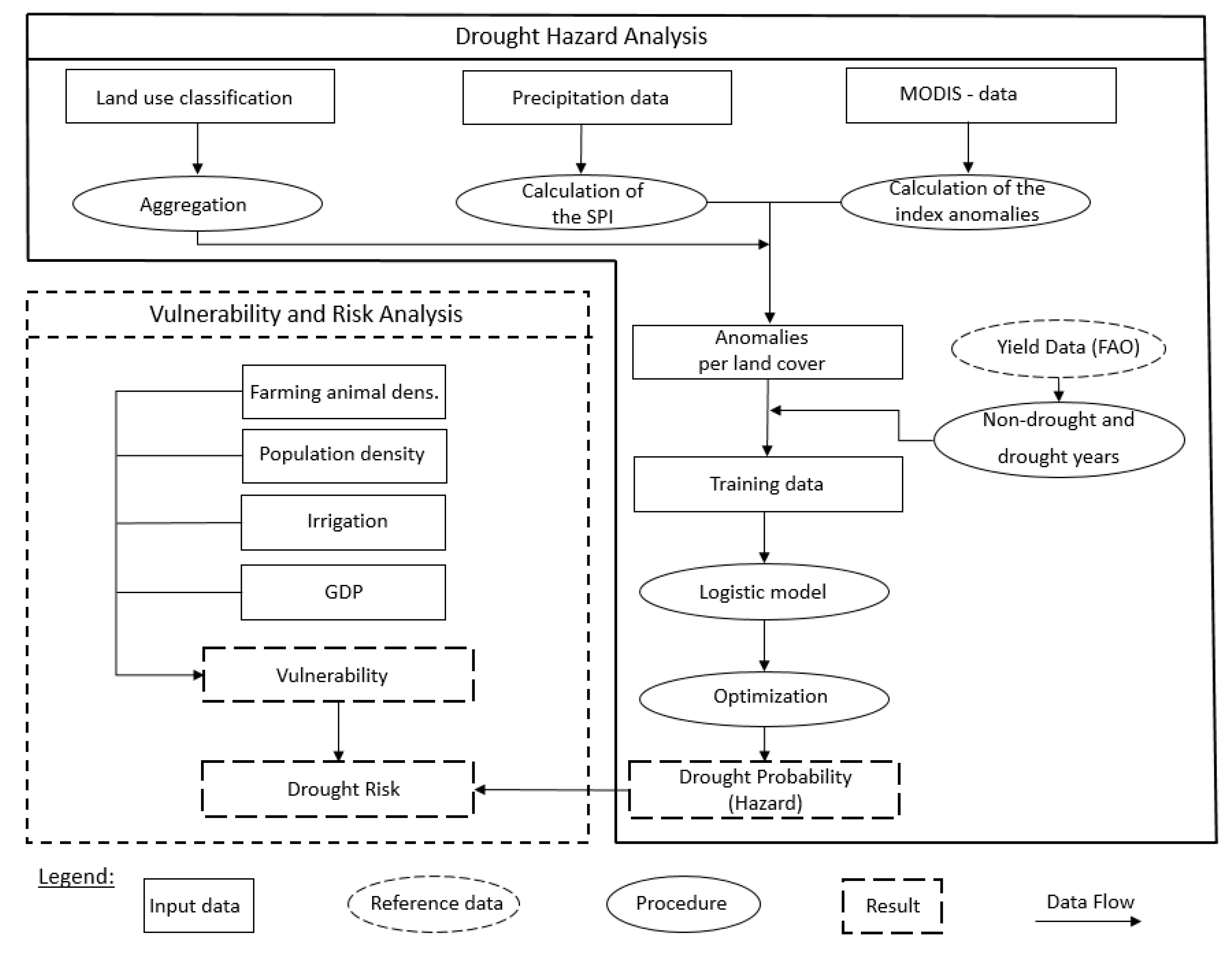
2.3.1. Drought Hazard Analysis

(1) Processing and Calculation of the Model Predictors

The precipitation data was used to produce the Standardized Precipitation Index (SPI), with the methodology from Mckee et al. [40]. The study at hand used the three-monthly SPI. For each month, rainfall data from the present month and the two previous months was accumulated from 1981 to 2017 before the SPI was calculated.

The MODIS data was processed differently for each product. The 8-day composites of the MOD09A1 product were corrected with the quality state flags to remove cloudy pixels. Subsequently, the Normalized Difference Vegetation Index (NDVI) [41] and the Normalized Difference Infrared Index (NDII) [22] were produced from the cloud masked MODIS bands between 2001 and 2017 at its original spatial resolution of 500 m. The indices were processed by calculating their monthly maxima and thus further reducing cloud influence [42]. The 8-day composites of the MOD11A2 product, on the other hand, were not corrected for clouds since the land surface temperature (LST) was only produced for cloud-free pixels [43]. Monthly maxima were also calculated for the LST. The 16-day composite MOD43A3 albedo product was selected on the 15th of each month and was assumed to be the monthly mean. From the MODIS albedo product, the mean of all three albedo bands (visual, near infrared, short wave infrared) was calculated and used as an input variable in this study.

In addition, index anomalies were produced to develop a normalized and spatially invariant measure that reduces the influence of spatially varying vegetation and land cover types. This was done for all MODIS-based indices used as model predictors (NDVI, NDII, LST, mean albedo). The anomalies were calculated as the deviation of the long-term mean standardized with the standard deviation (“z-score”) [22]:

$$Z_{kxy}=\frac{\left(D{I}_{kxy}-{\alpha }_{kx}\right)}{{\sigma }_{kx}},$$

(1)

Z_kxy represents the anomaly value for kernel k during the time span x, which was 2001–2017 in this study, for a given month y. DI_kxy stands for the drought index value for kernel k during the time span x in month y and α_kx und σ_kx represent the mean and standard deviation of kernel k over the time span x. The index anomalies were then used as predictors for the logistic regression model.

(2) Identification of Drought Periods

After the vegetation and rainfall index anomalies were derived, they were masked with the aggregated land use classification (Figure 1). Subsequently, drought and non-drought periods were determined within the growing periods of the main crops maize, green maize, sorghum, soybean, and wheat. For the USA, the growing season was assumed to last from May to September and for southern Africa from November to March. Drought periods were identified as drought seasons or drought years, using a segmented regression of the FAO’s annual yield data [29]. Long term shifts in the total yield are possible for example due to advances in technologization, widespread use of fertilizers or the implementation of irrigation. To consider these shifts in the modeling framework, the regression divided the time series into several segments and assigned a stable regression relationship to each segment [44]. Considering a standardized linear regression model

$$y_i=x_i\ast {\beta }_i+u_i\left(i=1,\dots ,n\right),$$

(2)

where y_i represents the estimate of the linear relationship of the response to x_i that includes the yield observations sorted by time i after applying ordinary least squares to the linear regression model. β_i represents the linear parameter estimates and u_i the constant. Assuming that there are m breakpoints, this model changes to

$$y_i=x_i\ast {\beta }_j+u_i\left(i=i_{j-1}+1,\dots ,i_j,j=1,\dots ,m+1\right),$$

(3)

where j represents the segment index. Zeileis et al. [44] developed an algorithm in “R”, a software environment for statistical computing, to automatically determine these breakpoints, which was used in this study. It was assumed that a segment would last a minimum of four years. This limits the total number of breakpoints for each crop type in each study area to three, given the assessed time period spans 2001 to 2017. Muggeo [45] transcribed the segmented regression model as a function in R that could be applied to the data using the breakpoints defined from the breakpoint analysis. In each study area, the residuals of the model for each crop type were subsequently determined individually and then accumulated. The five crops used in this study stand as representatives for the total agricultural yield in the three study areas. The standard deviation was calculated from the summed residuals in each region. The growing periods where residuals fell below one negative standard deviation were defined as drought years or periods. Non-drought years were periods in which the residuals exceeded one positive standard deviation. Any growing periods with values with a standard deviation between −1 and 1 were not considered, in order to ensure clean and distinctive training classes for the model. As a result, the drought years identified for model parametrization were only those years where a large-scale drought caused yield deficits and which affected the entire country during each respective growing period. A potential effect of yield losses caused by floods, pests or diseases (other than drought effects) in the training data was minimized by considering not only one crop type to determine drought, but rather five crop types. Since national yearly yield statistics for five crop types were used to identify a drought year, potential effects from small scale yield losses of non-drought causes on the training data are minimized. The drought and non-drought periods identified between 2001 and 2010 served as training data for the logistic regression model described in the following section.

(3) Logistic Regression Model

Binary logistic modeling has been successfully proven in numerous studies using remote sensing variables as predictors. Such models are also known to render robust variable relevancies, when correlation among variables is accounted for [46,47].

For the identified drought and non-drought years, monthly anomaly data from the NDVI, NDII, LST, albedo and 3-month SPI data were extracted for the relevant land use classes in the 2001–2010 training period for all months of the growing season. 2011 to 2017 was used to test the model. The anomalies were resampled to a spatial resolution of 0.01° and used as predictors for the logistic regression model (Figure 1). Thus, each pixel classified as agricultural, grass or bushland was defined as either a drought or a non-drought observation within the entire study area over the entire respective crop growing season. A random sample of 100,000 pixels (=observations) was taken per class (drought or non-drought) as training data.

Subsequently, the five input indices were tested for autocorrelation and multicollinearity using a Pearson correlation matrix and the condition index. Dormann et al. [48] suggest that a threshold of 0.7 in the pairwise Pearson correlation matrix indicates variables that strongly influence the model. For the condition index, values that exceed a value of 30 are considered critical and indicate strong multicollinearity [48]. Only variables that exhibited no multicollinearity according to the Pearson correlation and the condition index were included in the model as predictors. A logistic model was used to predict a binary classification of the dependent variable y (drought or non-drought). The probability produced by the logistic model with values between 0 and 1 were considered to be drought hazard. The calculation of the probability values p(X), that are translated into drought hazard, are defined using the logistic function [49]:

$$p\left(X\right)=\frac{e^{\beta 0+\beta 1X}}{1+e^{\beta 0+\beta 1X}},$$

(4)

with a linear regression function as basis [49]:

$$p\left(X\right)={\beta }_0+{\beta }_{1}X$$

(5)

After setting up the model, the z and p values of the individual predictors were analyzed. High z values (>|+/−2|) indicate a decisive influence of the variable on the modeling results. This finding can be confirmed with significant p values (<0.01) [49].

To evaluate the goodness of fit for the logistic regression model McFadden’s Pseudo R² was used [50]:

$$R_{MF}^2=1-\frac{l_M}{l_0},$$

(6)

l_M represents the log-likelihood of the estimated model and l₀ the log-likelihood of the zero model, which consists of only one constant. Values greater than 0 indicate predictive qualities of the model, while 1 reflects a perfect predictive power [50]. The values of McFadden’s Pseudo R² are generally much lower than those of the R² of general linear regression models. Values between 0.2 and 0.4 indicate an excellent model fit for McFadden’s Pseudo R² [51].

(4) Verification of the model results

In addition to the statistical evaluation described above, the model was also checked for plausibility. The Missouri Basin study area in the USA was the only site, where an operational drought model (USDM) was available. The USDM is recognized as an advanced tool for drought monitoring in science (e.g., [12]). The data is produced by the National Drought Mitigation Center of the University of Nebraska-Lincoln, the United States Department of Agriculture, and the National Oceanic and Atmospheric Administration and is available on the USDM’s homepage (http://droughtmonitor.unl.edu/Data/Datadownload/ComprehensiveStatistics.aspx). A visual comparison between the USDM maps and those produced by the logistic regression model provided a qualitative assessment of the model’s plausibility.

Due to the lack of spatial drought information besides global drought models, the verification in South Africa and Zimbabwe was based on newspaper reports and reports from aid agencies published in the World Wide Web (e.g., BBC News) about time periods and areas affected by drought. In addition, model results were compared against occurrence information of El Niño events, as teleconnections of the El Niño phenomenon are known to cause drought in southern Africa [52]. By comparing the data to the teleconnections caused by the El Niño and the drought reports, the model plausibility was assessed for Zimbabwe and South Africa. Finally, the model output was also compared to the Global Drought Observatory provided by the Joint Research Center (JRC) with the key input variables derived from meteorological, soil moisture and vegetation greenness data for drought hazard, population data and baseline water stress for drought exposure and social, economic and infrastructural factors like the level of well-being of individuals for vulnerability. Additionally, we used food security classification data from the Famine Early Warning Systems Network (FEWS NET) for Zimbabwe as a cross-verification source for the drought hazard model.

2.3.2. Vulnerability and Risk Analysis

A simplified drought risk analysis was performed by calculating a drought risk indicator, where risk is the product of vulnerability and hazard [53]. Drought hazard is defined as the probability of a drought occurring, which was calculated by the logistic regression model, while the vulnerability is a relative measure that indicates the degree to which a system is susceptible to damage from the onset of the harmful phenomenon (e.g., drought) [54].

The factors influencing the drought vulnerability in this study were the proportion of irrigated land, the gross domestic product per area, the population density and the density of grazing animals (cattle, sheep, goats). Areas with a higher gross domestic product indicate a lower drought vulnerability. Population density above 300 inhabitants per km² [55], urban areas and pixels immediately adjacent to urban areas were excluded from the analysis since we were only looking at crop- and rangeland. Each individual variable was normalized for each study area as follows:

$$y_i=\frac{x_i-x_{min}}{x_{max}-x_{min}},$$

(7)

whereby y_i is the focused standardized value, x_i is the observed value and x_min and x_max are the minimum and maximum of all observation values, respectively. Once the mean is calculated for these standardized variables, the drought vulnerability index (DVI) can be calculated using the following equation:

$$DV{I}_i=\frac{(1-I{L}_i)+\left(1-GD{P}_i\right)+P{D}_i+GA{D}_i}{4},$$

(8)

where IL, GDP, PD and GAD represent the mean of irrigated land, gross domestic product, population density and grazing animal density, respectively. The DVI represents the drought vulnerability and was used as a relative, spatial comparison to identify vulnerable areas. The different input variables for DVI can also be differently weighted if necessary. Drought risk was also just used as a relative measure assessed by the multiplication of DVI and drought hazard. This is due to the fact, that drought vulnerability and drought risk are highly complex and cannot be investigated in detail by including every aspect affecting them within this study. A future combination of the drought hazard model with other existing methods and models on drought vulnerability is possible.

3. Results

3.1. Drought Hazard Analysis in the USA, South Africa and Zimbabwe

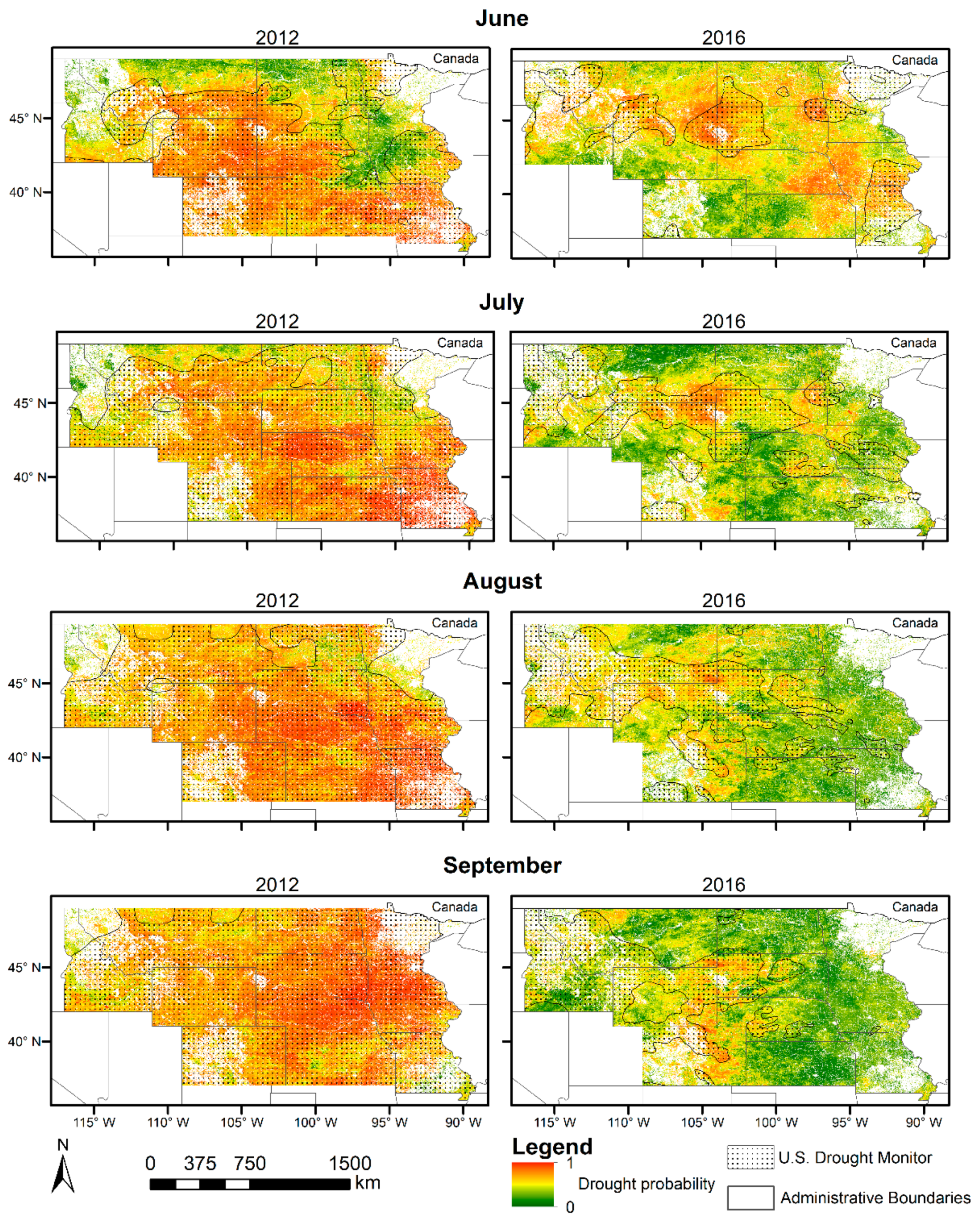
3.1.1. Drought Hazard in the Missouri Basin (USA)

As stated, the development of the logistic modeling and the construction of the method was first performed in the USA before they were transferred and adapted to South Africa and Zimbabwe. The segmented regression (see Section 2.3.1) showed that 2002 was the only drought year detected in the USA for the training data period from 2001 to 2010, and that 2004 and 2009 were non-drought years. The pairwise autocorrelation (

Table 2. Pairwise Pearson correlation of the model input variables for the model in the USA.

	SPI3	NDII	NDVI	Albedo
NDII	0.41	-	-	-
NDVI	0.45	0.71	-	-
Albedo	−0.3	−0.07	−0.24	-
LST	−0.56	−0.53	−0.49	0.22

) showed a critical Pearson correlation coefficient of 0.71 between the NDVI and NDII. Due to a slightly higher value in the explained variance for the highest condition index (

Table 3. Decomposed variances of the condition index for the model in the USA (only values >0.3 are shown).

Condition Index	Albedo	LST	NDII	NDVI	SPI3
1	-	-	-	-	-
1.75	-	-	-	-	-
3.15	0.49	0.57	-	-	-
4.23	-	-	-	-	0.96
10.66	-	-	0.93	0.94	-

) the NDVI was excluded as an input variable for the model.

The summary of the model output (

Table 4. Summary of the logistic regression model for the USA.

	Coefficient	z-Value
(constant)	−0.20	−35.6
Albedo	0.13	22.6
LST	0.43	66.6
NDII	−0.83	−111.7
SPI3	−0.12	−17.6

) shows z-values higher than |2| for all predictors with a confidence level of 99%, indicating that all variables have a significant influence and should be included in the logistic regression model. Moreover, McFadden’s Pseudo R² was found to be 0.16, which suggests a good fit.

2012 was identified as a drought year for the model application after the training data period (Figure 2). The maps of the calculated probabilities for 2012 showed increasing drought intensity while the affected area was also growing, finally covering almost the entire area of the Missouri Basin except for the southeast and northwest parts in September. In 2016, drought probabilities decreased over the course of the growing season. Towards the end of the crop cultivation period, high drought probabilities can only be seen in smaller areas in the center and south of the Missouri Basin. On the contrary, low drought probabilities, i.e., normal conditions for agricultural land, grass- and shrubland, were spread over most of the study area. Although not identical, both the model results and the US Drought Monitor indicate large areas affected by drought in 2012 that spatially match. Differences between the two drought models were more pronounced in the 2016 non-drought year.

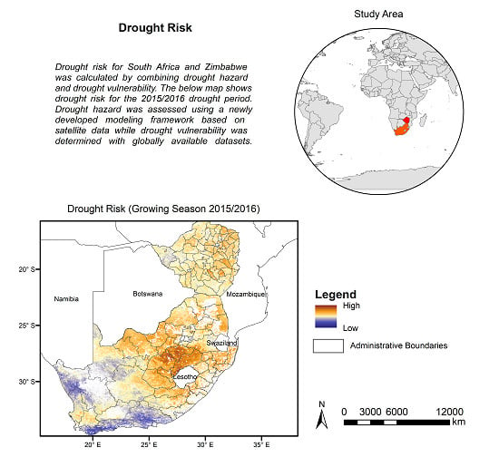
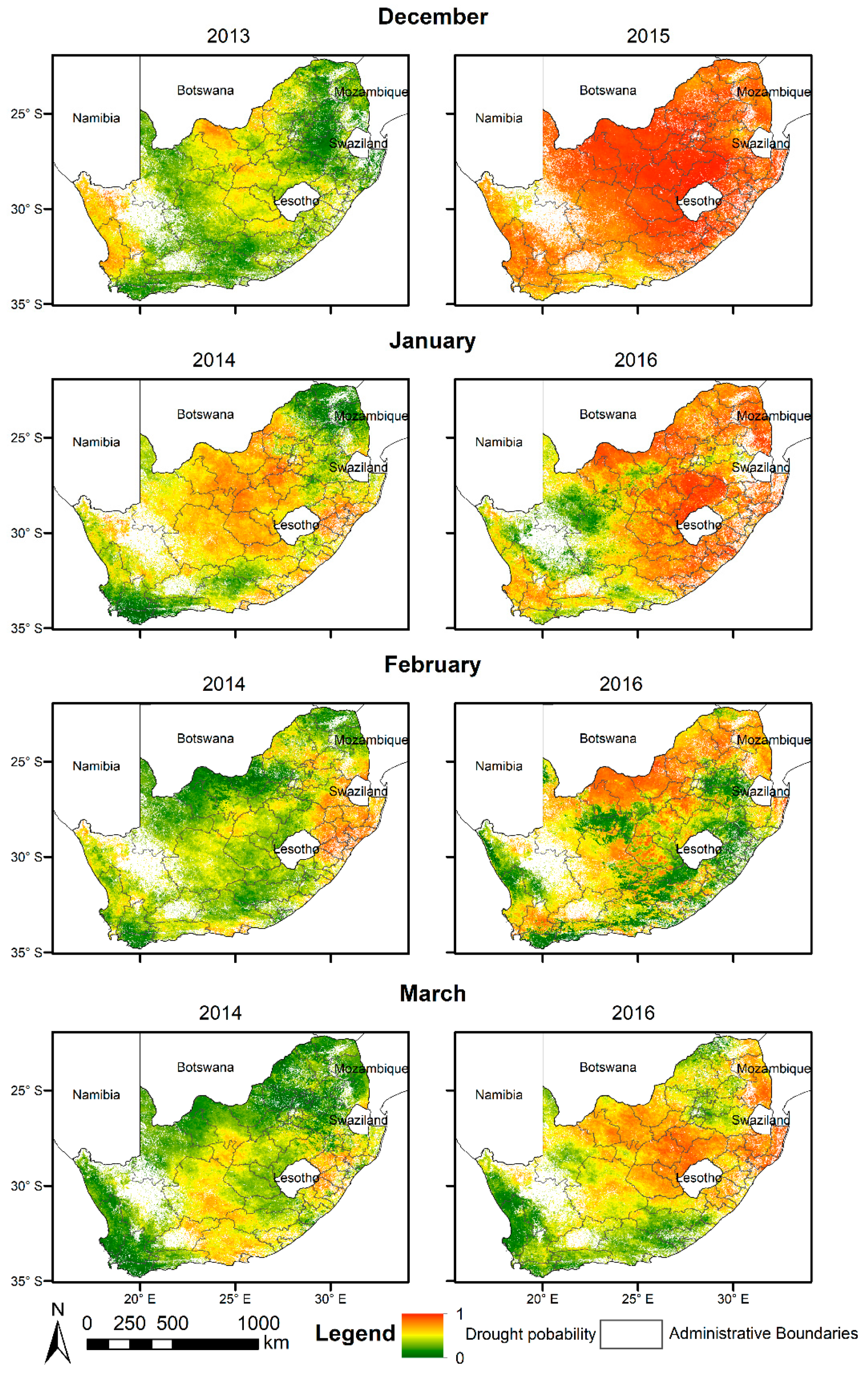
3.1.2. Applicability of the Developed Hazard Model for South Africa

The analysis over South Africa identified 2007 as a drought year and the years 2002 and 2009 as non-drought years over a time period from 2001 to 2010. The pairwise autocorrelation in South Africa does not show any Pearson correlation values higher than 0.7 and the Condition Index is also well below the critical value. As such, all variables were used to model drought probabilities in South Africa. As with the model results for the USA, all predictors showed z-values greater than |2| on a significance level of 99% (

Table 5. Summary of the logistic regression model for South Africa.

	Coefficient	z-Value
(constant)	−0.17	−31.5
Albedo	0.25	40.0
LST	0.48	59.8
NDII	−0.35	−40.2
NDVI	0.61	70.0
SPI3	−0.93	−118.1

). The model for South Africa also showed a good model fit, with a McFadden’s Pseudo R² value of 0.17.

In order to exemplarily compare the hazard model prediction for a drought and a non-drought year for South Africa, the 2013/2014 growing period (hereinafter referred to as 2014) was chosen as the non-drought period and 2015/2016 (hereinafter referred to as 2016) as the drought period (Figure 3). A comparison of the individual months clearly showed that high drought probability areas were more widespread and frequent in 2016. In the non-drought year, higher probabilities were only found in the center of the country in January 2014. Low to medium probability ranges were distributed over the entire growing season. During the drought period, one can see that high drought probabilities were prevalent over most of the country in December 2015, followed by a decrease over the subsequent months. In February 2016, artefacts caused by errors in the MODIS cloud mask can be seen in the center and south of South Africa.

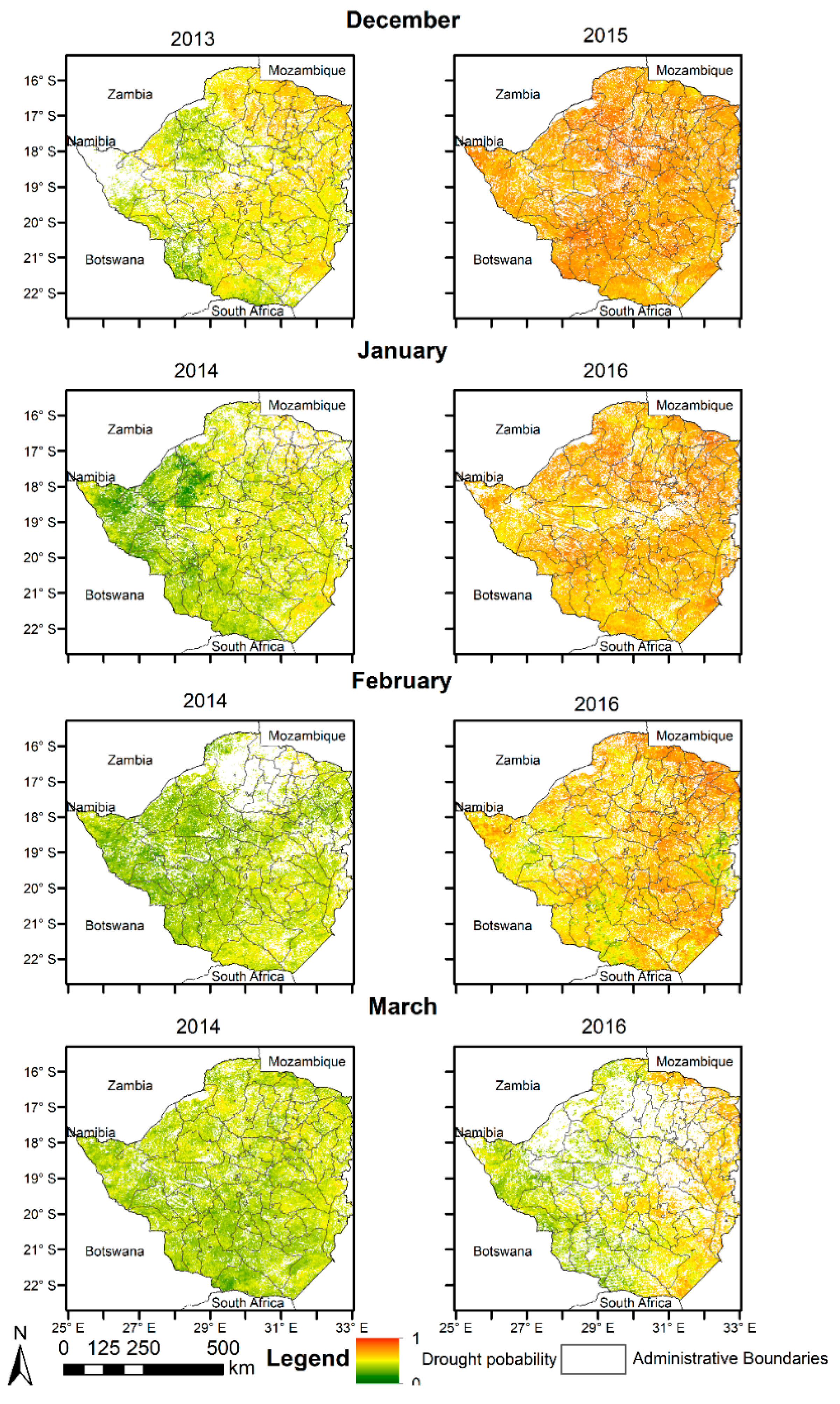
3.1.3. Applicability of the Developed Hazard Model in Zimbabwe

In Zimbabwe, 2003, 2005 and 2008 were identified as drought years, while 2004 and 2006 were identified as non-drought years. Neither the pairwise autocorrelation nor the Condition Index showed critical values and all predictors had a high and significant impact on the model results according to their z-values (

Table 6. Summary of the logistic regression model in Zimbabwe.

	Coefficient	z-Value
(constant)	−0.03	−6.3
Albedo	0.19	−35.4
LST	0.07	−10.1
NDII	−0.46	−67.4
NDVI	0.10	18.2
SPI3	−0.38	−57.3

). In contrast to the results for South Africa and the USA, the Pseudo R² values obtained for Zimbabwe was 0.06, which indicates a moderate predictive quality.

The drought probabilities calculated for the 2013/2014 (non-drought) and 2015/2016 (drought) growing periods in Zimbabwe reveal differing climatic conditions (Figure 4). Similar to the conditions seen in South Africa, the latter period is a drought year while the model clearly identified 2014 as a non-drought year. In general, drought probability in Zimbabwe was higher in 2016 than in 2014 and the probabilities decreased over the growing periods of both years.

3.1.4. Evaluation of the Logistic Regression Model for South Africa and Zimbabwe

The advanced monitoring system of the USDM is not available in other countries like South Africa or Zimbabwe. Therefore, both, newspaper articles and drought reports, as well as data on the past El Niño event in 2015/2016 were used for evaluation. The known teleconnections of El Niño are hot and dry conditions between December and February in the southeastern part of Africa [56]. The Oceanic Nino Index (ONI) registered a strong El Niño event during the 2015/2016 season [57] and its effect can be seen in the model results of South Africa and Zimbabwe. The drought probabilities predicted by the logistic regression model were highest during this event, as seen prominently in the North and East of South Africa. In Zimbabwe it seems, that all areas were equally affected in the same period. A decrease in drought probabilities was also observed at the beginning of 2016 in both countries which complies with ONI’s reported maximum at the end of 2015, followed by a steadily decreasing trend thereafter.

Newspapers also reported on the 2015/2016 drought in South Africa. According to BBC News [58] and Al Jazeera [59], all provinces in the East of the country like Free State, KwaZulu-Natal and Limpopo, were severely affected. These reports were consistent with the known teleconnections of an El Niño event. The hazard model results for South Africa corroborates both the reports and the climate patterns in these regions (Figure 3). The conditions in Free State and KwaZulu-Natal also lasted longer than in other regions, which is consistent with the newspaper reports claiming that these two provinces were the most affected. News24 [60] also reported extreme drought on the South African West Coast in January 2016, along with a high fire risk. This coincides with the high drought probabilities predicted for the end of 2015 and the beginning of 2016. Overall, the newspaper reports on the 2015/2016 drought and the El Niño data during the same period provide qualitative evidence that the model results resemble true conditions on the ground.

In Zimbabwe, BBC News [61] and ReliefWeb [62] both reported prevailing drought conditions in the months prior to February 2016. They cited various provinces and regions that were particularly affected, such as Hwange, Masvingo or Matabeleland South and Matabeleland North, concluding that most of the country was affected by drought. The modeled drought probability maps predicted herein corroborate this, showing high drought probabilities across the country over the same period. The results of the drought hazard model for February 2016 were also compared to FEWS NET food security classification data and drought risk data from the Global Drought Observatory (Figure 5). The visual comparison shows high drought hazard patterns across the country going along with middle to high food insecurity and middle to high drought risk. The visual agreement within this cross-verification shows the plausibility of the drought hazard model.

In the observation period from 2011 to 2017, there were only reports for one wide spread drought event (2015–2016). Accordingly, the other years were considered as years with no widespread drought in both countries. Overall, the model output proved to be well suited to predict drought probabilities for agro-ecological landscapes in southern Africa.

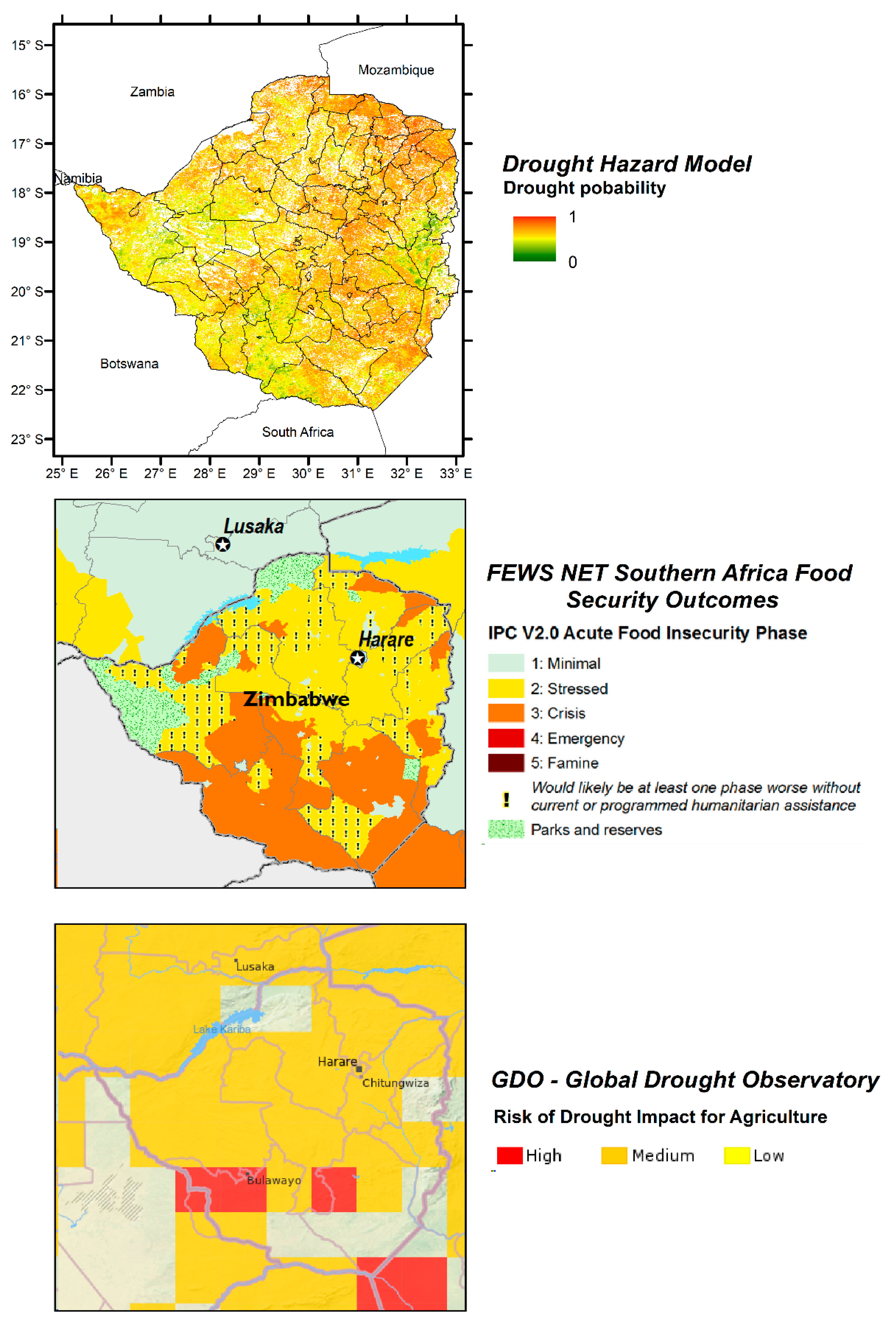
3.1.5. Comparison between the Drought Hazard Model and the Global Drought Observatory of the Joint Research Center (JRC)

Currently, there is no known approach that utilizes remote sensing variables to predict drought hazard and has been validated against a state-of-the art drought monitoring system. A method to predict drought hazard, vulnerability and risk in data scares areas like Zimbabwe is also missing. However, the model presented does share similarities with the GDO’s Risk of Drought Impacts for Agriculture (RDrI-Agri) product which combines drought hazard, vulnerability and exposure [26].

The comparison with the RDrI-Agri was done visually (see Figure 5 for an example) since the difference in the spatial resolution thus not allow for a pixel by pixel analysis. Both datasets predicted similar results for the 2013/2014 and the 2015/2016 growing seasons in South Africa and Zimbabwe. The 2013/2014 season showed low RDrI-Agri and low modeled hazard values while the 2015/2016 season displayed high RDrI-Agri and high hazard values. For 2016 there was, however, a slight discrepancy in drought risk and hazard intensity values that may be due to the differences in input model variables and areas under consideration.

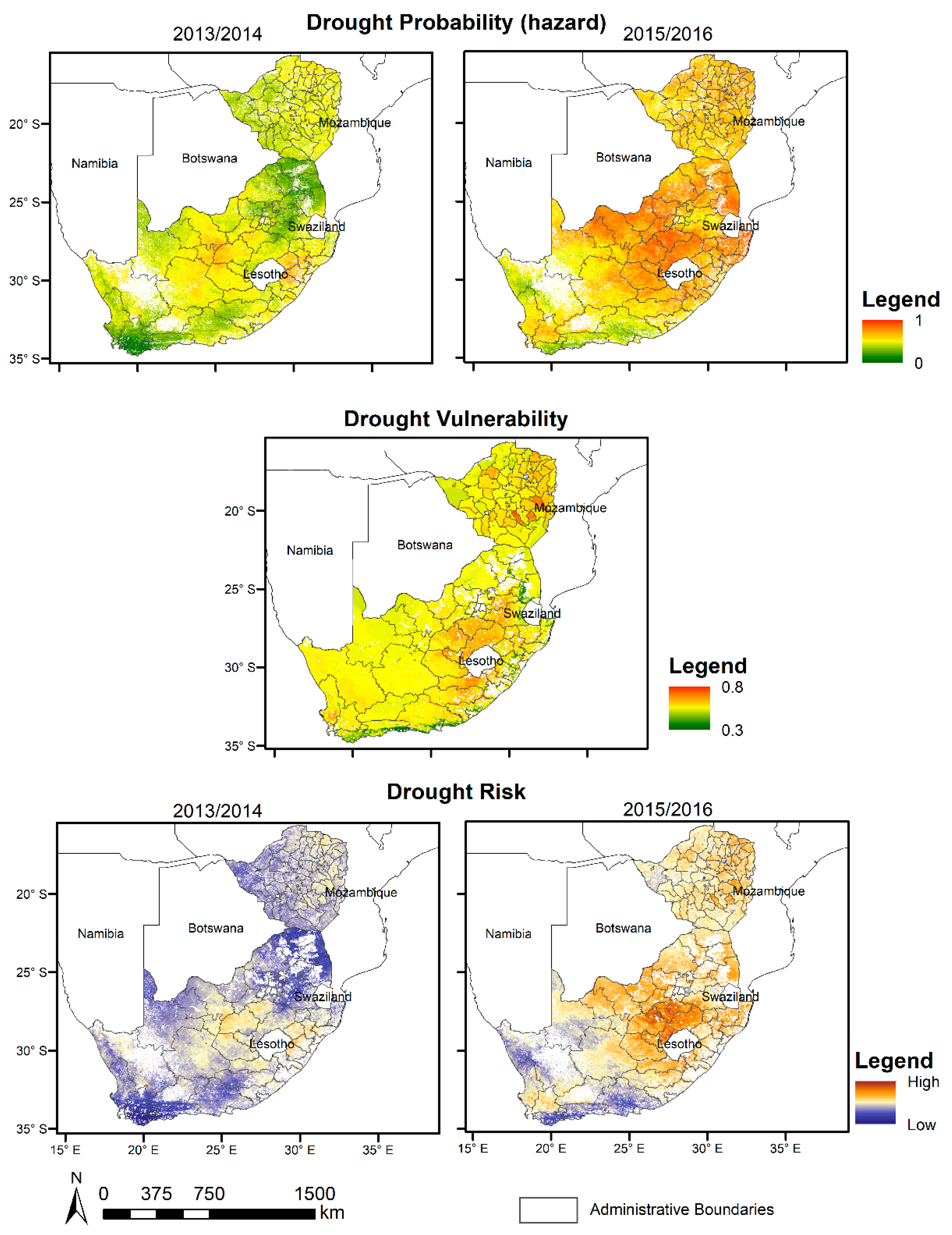
3.2. Drought Vulnerability and Risk Analysis in South Africa and Zimbabwe

Figure 5 shows low drought vulnerabilities along the southern coast of Africa and parts of eastern South Africa, as well as in western Zimbabwe. The southeastern part of Zimbabwe also showed some isolated areas with lower drought vulnerabilities over the observation period which could be due to irrigated croplands. The most vulnerable regions were Free State and KwaZulu-Natal in South Africa and the provinces around Masvingo like Chivi and Buhera in Zimbabwe.

A comparison of the two growing periods for South Africa and Zimbabwe showed clear differences in drought risk. In 2013/2014, low drought risk values were visible over larger areas in South Africa and Zimbabwe while the vulnerability was constant over the full observation period. On the contrary, for the drought within 2015/2016, a greater drought risk could be predicted over a larger area. The most vulnerable regions in both countries are also clearly discernable in the risk maps for both years.

4. Discussion

The model produced spatially explicit information on drought hazard, drought vulnerability and drought risk that performed well according to the quantitative and plausibility checks.

In the comparison with the Global Drought Observatory, there were some discrepancies in the intensity of drought risk and drought hazard which could be due to the diverging methods used. In the RDrI-Agri model, the risk of drought impact on agriculture is predicted while the model presented here predicts drought hazard probabilities on agricultural and rangeland. This presented model also runs on a spatial resolution of 0.01° which is more detailed than the RDrI-Agri model’s 1°. On the other hand, the RDrI-Agri model offers a higher temporal resolution, producing maps every 10 days instead of each month. The drought risk product presented here, could not be compared to the RDrI-Agri model because our drought risk model result only considers crop growing seasons’. Due to the complexity of drought effects and impacts, validation of drought models is difficult in general. The presented quantitative figures of model’s McFadden’s Pseudo R², p values, however, demonstrated the the plausibility of the results. Hagenlochner et al. [54] stated that less than 20% of their reviewed drought studies have conducted any form of validation or evaluation of their results. Considering that lack of validation methods and the lack of reference data we used a variety of available information and data to cross-verify our results. Even though this could not be done in a quantitative way, this alternative cross-verification approach showed to be effective for model plausibility checks.

The spatial transferability of our approach is generally possible since we are using globally available FAO yield response data (as response variables) combined with globally available remote sensing data as predictors. However, the method should be used with care for regions where strong and large-scale yield anomalies are caused by factors different from drought. The logistic regression model that was developed (trained) for the Missouri Basin, could be successfully applied to South Africa and Zimbabwe, thus further demonstrating the transferability of the hazard modeling approach. The application of the model should run at country level, since the FAO yield data is only available at this spatial unit. It is also important to mention that the model itself needs to be country-specifically calibrated and set up when being transferred but always based on the same input data. When setting up the model, multicollinearity should also be checked and minimized during the model optimization process. The final model equation can also contain different variable relevancies depending on the country or region. The need for a country-specific set up becomes apparent when comparing drought and non-drought years using the FAO stats yield data. When considering the three countries USA, Zimbabwe and South Africa, the same crops could be used for the analysis due to their similar agricultural use and responses to water stress in the three countries. However, this may not be the case in other areas, such as Asia, where different reference crops should be selected that better mimic water stress responds. Kogan [63] analyzed the relationship between vegetation health and crop yields in different countries around the world and found, that yield modeling with the help of the vegetation health indices differs regionally for different crops. Thus, regarding the global applicability of our modeling framework, geographical location, climate zone and crop type differences must be considered, specifically when selecting drought and non-drought years in the time line reference yields data. The segmented regression, which mainly accounts for effects of technological advances on yields, can be simply transferred to other crop yields data or other regions. Due to regional differences in climate and plant characteristics, the herein considered variables Albedo, LST, NDII, NDVI and SPI3 vary in importance in terms of their relevance to drought hazard. This results in different model equations for every region when applying the model after a country-specific set-up. The changing relevance of the input variables per country also relates to the autocorrelation and the z-values of the model variables. In South Africa and Zimbabwe, for example, no critical values were found in the pairwise autocorrelation in contrast to the USA. This is due to regional deviating plant characteristics leading to changes in the indices and their interplay [64]. For example, the SPI3 with a z-value of 17.6 is significantly less influential for the model in the USA than it is in South Africa (118.1) and Zimbabwe (57.3). One possible explanation is that the dependence of plants on precipitation could be more distinct in South Africa and Zimbabwe due to, for instance, the lower spatial coverage of irrigation croplands in these two countries [38]. This becomes clearer when looking at the importance of the NDII in the model of the three countries. Di Wu et al. [12] stated that the NDII in its analysis is sensitive to the detection of droughts over irrigated fields. In a country like the USA, where a large part of the agricultural area is under irrigation [12], this index thus plays a decisive role in modeling the probability of drought. The comparison of the z values for the NDII suggests a similar trend. In the USA this was 111.7 and was thus significantly higher than the values of 40.2 and 67.4 in South Africa and Zimbabwe, respectively. Concluding this section, the model showed to be spatially transferable while also capturing regional drought relevant impacts and effects and thus providing spatially more precise information compared to global drought models.

In contrast to existing country statistics on income, poverty or food availability, the vulnerability analysis presented here is simplified but spatially explicit while helping to support drought preparedness or water resource management of more vulnerable regions or communities [26]. As apparent in Figure 6, the administrative units at which level population, GPD and animal density data are reported for Zimbabwe and South Africa, are clearly visible in the vulnerability analysis results. These data that are aggregated information at administrative unit level, can cause under- or overestimation of drought risk in some areas. For instance, in the Kruger National Park (KNP) in northeastern South Africa on the border to Mozambique, this becomes apparent. Within the KNP, high per pixel vulnerability scores are predicted although the Kruger Park can be considered a ‘no vulnerability’ area with regard to GDP, population, livestock or irrigation. Moreover, if one compares South Africa and Zimbabwe, the spatial patterns in Zimbabwe are more easily delineated than in South Africa (Figure 5). This is probably due to the fact that spatially explicit data availability in South Africa regarding to population density, GDP and livestock density is generally much better than in Zimbabwe.

To support drought preparedness and interventions, the vulnerability and simplified risk modeling framework allows for spatial comparisons between regions and can be most useful to identify drought prone regions that are in danger of damages or economic losses [65]. Ebi & Bowen [66] noted that the increase in drought exposure is accompanied by a decline in the Human Development Index. This suggests the need for an approach that allows for a comparison of vulnerability and risk between countries. A disadvantage of this analysis approach is essentially that no absolute degree of vulnerability and risk can be determined. Other studies on regional vulnerability incorporate a wide spectrum of variables to determine drought vulnerability and thus better reflect the absolute drought vulnerability. Vulnerability dimensions are mentioned by Hagenlochner et al. [54] in their review article on drought assessment. The main obstacle is the availability of global spatially explicit data sets. Since only a few useful data sets are available for some countries in this form, water supply and availability could not be included. In our models, the separate analysis of grazing animals offers additional variable weighting possibilities. All input index variables can be weighted differently and the vulnerability index can be easily extended with new data sets that may be available in the future. This allows a better understanding of the region-specific significance of the individual factors for agriculture and pasture management and a more appropriate calculation of drought vulnerability and risk. In this context, it was demonstrated that the simplified analysis of vulnerability and risk can be feasibly calculated at the country level.

5. Conclusions

This paper presented a satellite data-driven logistic regression model that can model drought hazard for agriculture, grass- and shrubland biomes while being spatially transferable. The model showed a good spatial agreement with the U.S. Drought Monitor when compared in the Missouri study site in both drought and non-drought years. The subsequent evaluation in South Africa and Zimbabwe with the help of drought reports and data on the last major El Niño event in 2015/2016 proved the predictive quality of the model. Considering the goodness of fit for the logistic regression model, McFadden’s Pseudo R² showed a good predictive quality for the USA and for South Africa, but only a moderate predictive quality for Zimbabwe. However, not only quantitative measurements are in need to assess the model performance, but also qualitative analyses regarding plausibility of results. The comparison to the Global Drought Observatory developed by the JRC and to the food security classification data provided by FEWS NET also showed a good match with the results obtained herein.

Overall, the logistic regression model shown here combines the advantage of global models with their global applicability with the strengths of regional models that allow for assessing drought hazard at a regional level through improved spatial resolution. This might require changing various input variables, weights and crop types affected by drought depending on different characteristics of the area. Although it has shown its potential for global transferability, further research on the suitability of the model to predict drought hazard in other geographic regions needs to be done. The drought hazard model can also be seen as a first step towards near real-time drought hazard monitoring since it is exclusively based on near real-time satellite data and thus reflects current conditions. This study could demonstrate a consistent way of analyzing drought hazard, risk and vulnerability within a country. In order to advance this methodology, new global and spatially explicit time series data is needed to support and provide a more comprehensive vulnerability analysis.

References

1. Wilhite, D.A. (Ed.) Drought: A Global Assessment, 2nd ed.; Routledge: London, UK, 2000; ISBN 9780415168335. [Google Scholar]
2. Sivakumar, M.V.K.; Motha, R.P.; Wilhite, D.A.; Wood, D.A. Agricultural Drought Indices. In Proceedings of the WMO/UNISDR Expert Group Meeting on Agricultural Drought Indices, Murcia, Spain, 2–4 June 2010. [Google Scholar]
3. UN-Spider. Drought. 2019. Available online: http://www.un-spider.org/risks-and-disasters/natural-hazards/drought (accessed on 3 December 2019).
4. IPCC (Ed.) Summary for Policymakers. In Climate Change 2013: The Physical Science Basis. Contribution of Working Group I to the Fifth Assessment Report of the Intergovernmental Panel on Climate Change; Cambridge University Press: Cambridge, UK, 2013. [Google Scholar]
5. Pachauri, R K.; Mayer, L. (Eds.) Climate Change 2014, Synthesis Report; Intergovernmental Panel on Climate Change: Geneva, Switzerland, 2015; ISBN 978-92-9169-143-2. [Google Scholar]
6. Wilhite, D.A. (Ed.) Preparing for Drought: A Methodology. In Drought: A Global Assessment, 2nd ed.; Routledge: London, UK, 2000; pp. 89–104. ISBN 9780415168335. [Google Scholar]
7. Owrangi, M.A.; Adamowski, J.; Rahnemaei, M.; Mohammadzadeh, A.; Sharifan, R.A. Drought Monitoring Methodology Based on AVHRR Images and SPOT Vegetation Maps. JWARP 2011, 3, 325–334. [Google Scholar] [CrossRef] [Green Version]
8. Wu, J.; Zhou, L.; Liu, M.; Zhang, J.; Leng, S.; Diao, C. Establishing and assessing the Integrated Surface Drought Index (ISDI) for agricultural drought monitoring in mid-eastern China. Int. J. Appl. Earth Obs. Geoinf. 2012, 23, 397–410. [Google Scholar] [CrossRef]
9. Zhou, L.; Wu, J.; Zhang, J.; Leng, S.; Liu, M.; Zhang, J.; Zhao, L.; Zhang, F.; Shi, Y. The Integrated Surface Drought Index (ISDI) as an Indicator for Agricultural Drought Monitoring: Theory, Validation, and Application in Mid-Eastern China. IEEE J. Sel. Top. Appl. Earth Obs. Remote Sens. 2013, 6, 1254–1262. [Google Scholar] [CrossRef]
10. Gulácsi, A.; Kovács, F. Drought Monitoring With Spectral Indices Calculated From Modis Satellite Images in Hungary. J. Environ. Geogr. 2015, 8. [Google Scholar] [CrossRef] [Green Version]
11. Zhuo, W.; Huang, J.; Zhang, X.; Sun, H.; Zhu, D.; Su, W.; Zhang, C.; Liu, Z. Comparison of five drought indices for agricultural drought monitoring and impacts on winter wheat yields analysis. In Proceedings of the 2016 Fifth International Conference on Agro-Geoinformatics (Agro-Geoinformatics), Tianjin, China, 18–20 July 2016; pp. 1–6. [Google Scholar] [CrossRef]
12. Di, W.; Qu, J.J.; Hao, X. Agricultural drought monitoring using MODIS-based drought indices over the USA Corn Belt. Int. J. Remote Sens. 2015, 36, 5403–5425. [Google Scholar] [CrossRef]
13. Zhang, Y.; Peng, C.; Li, W.; Fang, X.; Zhang, T.; Zhu, Q.; Chen, H.; Zhao, P. Monitoring and estimating drought-induced impacts on forest structure, growth, function, and ecosystem services using remote-sensing data: Recent progress and future challenges. Environ. Rev. 2013, 21, 103–115. [Google Scholar] [CrossRef]
14. Hazaymeh, K.; Hassan, Q.K. Remote sensing of agricultural drought monitoring: A state of art review. AIMS Environ. Sci. 2016, 3, 604–630. [Google Scholar] [CrossRef]
15. Peng, C.; Deng, M.; Di, L. Relationships between Remote-Sensing-Based Agricultural Drought Indicators and Root Zone Soil Moisture: A Comparative Study of Iowa. IEEE J. Sel. Top. Appl. Earth Obs. Remote Sens. 2014, 7, 4572–4580. [Google Scholar] [CrossRef]
16. Park, S.; Im, J.; Park, S.; Rhee, J. Drought monitoring using high resolution soil moisture through multi-sensor satellite data fusion over the Korean peninsula. Agric. For. Meteorol. 2017, 237–238, 257–269. [Google Scholar] [CrossRef]
17. Zhang, Q.; Yu, H.; Sun, P.; Singh, V.P.; Shi, P. Multisource data based agricultural drought monitoring and agricultural loss in China. Glob. Planet. Chang. 2019, 172, 298–306. [Google Scholar] [CrossRef]
18. Bayissa, Y.A.; Tadesse, T.; Svoboda, M.; Wardlow, B.; Poulsen, C.; Swigart, J.; van Andel, S.J. Developing a satellite-based combined drought indicator to monitor agricultural drought: A case study for Ethiopia. GIScience Remote Sens. 2019, 56, 718–748. [Google Scholar] [CrossRef]
19. Zhang, X.; Obringer, R.; Wei, C.; Chen, N.; Niyogi, D. Droughts in India from 1981 to 2013 and Implications to Wheat Production. Sci. Rep. 2017, 7, 44552. [Google Scholar] [CrossRef] [PubMed] [Green Version]
20. Sur, C.; Park, S.-Y.; Kim, T.-W.; Lee, J.-H. Remote Sensing-based Agricultural Drought Monitoring using Hydrometeorological Variables. KSCE J. Civ. Eng. 2019, 23, 5244–5256. [Google Scholar] [CrossRef]
21. Qu, C.; Hao, X.; Qu, J.J. Monitoring Extreme Agricultural Drought over the Horn of Africa (HOA) Using Remote Sensing Measurements. Remote Sens. 2019, 11, 902. [Google Scholar] [CrossRef] [Green Version]
22. Caccamo, G.; Chisholm, L.A.; Bradstock, R.A.; Puotinen, M.L. Assessing the sensitivity of MODIS to monitor drought in high biomass ecosystems. Remote Sens. Environ. 2011, 115, 2626–2639. [Google Scholar] [CrossRef]
23. Chang, C.-T.; Wang, H.-C.; Huang, C.-Y. Assessment of MODIS-derived indices (2001–2013) to drought across Taiwan’s forests. Int. J. Biometeorol. 2017, 1–14. [Google Scholar] [CrossRef] [PubMed]
24. Wan, Z.; Wang, P.; Li, X. Using MODIS Land Surface Temperature and Normalized Difference Vegetation Index products for monitoring drought in the southern Great Plains, USA. Int. J. Remote Sens. 2004, 25, 61–72. [Google Scholar] [CrossRef]
25. Wang, S.; Davidson, A.; Latifovic, R.; Trishchenko, A. The impact of drought on land surface albedo. Am. Geophys. Union 2004, 85. [Google Scholar]
26. Vogt, J.V.; Naumann, G.; Masante, D.; Spinoni, J.; Cammalleri, C.; Erian, W.; Pischke, F.; Pulwarty, R.; Barbosa, P. Drought Risk Assessment. A Conceptual Framework; Publications Office of the European Union: Luxembourg, 2018; ISBN 978-92-79-97469-4. [Google Scholar]
27. Huntington, J.L.; Hegewisch, K.C.; Daudert, B.; Morton, C.G.; Abatzoglou, J.T.; McEvoy, D.J.; Erickson, T. Climate Engine: Cloud Computing and Visualization of Climate and Remote Sensing Data for Advanced Natural Resource Monitoring and Process Understanding. Bull. Am. Meteorol. Soc. 2017, 98, 2397–2410. [Google Scholar] [CrossRef]
28. Chen, D.; Chen, H.W. Using the Köppen classification to quantify climate variation and change: An example for 1901–2010. Environ. Dev. 2013, 6, 69–79. [Google Scholar] [CrossRef]
29. FAO. Faostat. 2019. Available online: http://www.fao.org/faostat/en/#data (accessed on 10 January 2019).
30. Homer, C.; Dewitz, J.; Yang, L.; Jin, S.; Danielson, P.; Xian, G.; Coulston, J.; Herold, N.; Wickham, J.; Megown, K. Completion of the 2011 National Land Cover Database for the Conterminous United States—Representing a Decade of Land Cover Change Information. Photogramm. Eng. Remote Sens. 2015, 81, 345–354. [Google Scholar]
31. ESA Climate Change Initiative—Land Cover project 2017. CCI Land Cover—S2 Prototype Land Cover 20M Map of Africa. 2016. Available online: http://2016africalandcover20m.esrin.esa.int/ (accessed on 14 March 2019).
32. Funk, C.; Peterson, P.; Landsfeld, M.; Pedreros, D.; Verdin, J.; Shukla, S.; Husak, G.; Rowland, J.; Harrison, L.; Hoell, A.; et al. The climate hazards infrared precipitation with stations—A new environmental record for monitoring extremes. Sci. Data 2015, 2, 150066. [Google Scholar] [CrossRef] [PubMed] [Green Version]
33. Vermote, E.F.; Roger, J.C.; Ray, J.P. MODIS Surface Reflectance User’s Guide—Collection 6. 2018. Available online: http://modis-sr.ltdri.org/guide/MOD09_UserGuide_v1.4.pdf (accessed on 20 April 2018).
34. Wan, Z.; Hook, S.; Hulley, G. MOD11A2 MODIS/Terra Land Surface Temperature/Emissivity 8-Day L3 Global 1 km SIN Grid V006 [Data]; NASA EOSDIS Land Processes DAAC; U.S. Geological Survey: Reston, VA, USA, 2015. [CrossRef]
35. Schaaf, C.; Wang, Z. MCD43A3 MODIS/Terra + Aqua BRDF/Albedo Daily L3 Global—500 m V006; NASA EOSDIS Land Processes DAAC; U.S. Geological Survey: Reston, VA, USA, 2015. [CrossRef]
36. CIESIN. Gridded Population of the World, Version 4 (GPWv4): Population Density, Revision 10. Available online: https://catalog.data.gov/dataset/gridded-population-of-the-world-version-4-gpwv4-population-density-revision-10 (accessed on 10 January 2019).
37. Kummu, M.; Taka, M.; Guillaume, J.H.A. Gridded global datasets for Gross Domestic Product and Human Development Index over 1990–2015. Sci. Data 2018, 5, 180004. [Google Scholar] [CrossRef] [Green Version]
38. Landmann, T.; Eidmann, D.; Cornish, N.; Franke, J.; Siebert, S. Optimizing harmonics from Landsat time series data: The case of mapping rainfed and irrigated agriculture in Zimbabwe. Remote Sens. Lett. 2019, 10, 1038–1046. [Google Scholar] [CrossRef]
39. Gilbert, M.; Nicolas, G.; Cinardi, G.; van Boeckel, T.P.; Vanwambeke, S.O.; Wint, G.R.W.; Robinson, T.P. Global distribution data for cattle, buffaloes, horses, sheep, goats, pigs, chickens and ducks in 2010. Sci. Data 2018, 5, 180227. [Google Scholar] [CrossRef] [Green Version]
40. Mckee, T.B.; Doesken, N.J.; Kleist, J. The Relationship of Drought Frequency and Duration to Time Scales. Eighth Conf. Appl. Climatol. 1993, 22, 179–184. [Google Scholar]
41. Rouse, J.W.; Hass, R.H.; Schell, J.A.; Deering, D.W. Monitoring Vegetation Systems in the Great Plains with ERTS. In Proceedings of the 3rd Earth Resources Technology Satellite-1 Symposium, Greenbelt, MD, USA, 10–14 December 1973; pp. 309–317. [Google Scholar]
42. Huete, A.; Didan, K.; Miura, T.; Rodriguez, E.P.; Gao, X.; Ferreira, L.G. Overview of the radiometric and biophysical performance of the MODIS vegetation indices. Remote Sens. Environ. 2002, 83, 195–213. [Google Scholar] [CrossRef]
43. Wan, Z. MODIS Land Surface Temperature Products Users’ Guide: Collection-6. 2019. Available online: https://icess.eri.ucsb.edu/modis/LstUsrGuide/MODIS_LST_products_Users_guide_Collection-6.pdf (accessed on 26 March 2019).
44. Zeileis, A.; Kleiber, C.; Krämer, W.; Hornik, K. Testing and dating of structural changes in practice. Comput. Stat. Data Anal. 2003, 44, 109–123. [Google Scholar] [CrossRef] [Green Version]
45. Muggeo, V.M.R. Segmented: An R package to fit regression models with broken-line relationships. R News 2008, 8, 20–25. [Google Scholar]
46. Abdel-Rahman, E.; Landmann, T.; Kyalo, R.; Ong’amo, G.; Mwalusepo, S.; Sulieman, S.; Le Ru, B. Predicting stem borer density in maize using RapidEye and generalized linear models. Int. J. Appl. Earth Obs. Geoinf. 2017, 57, 61–74. [Google Scholar] [CrossRef]
47. Mosomtai, G.; Evander, M.; Sandström, P.; Ahlm, C.; Sang, R.; Hassan, O.A.; Affognon, H.; Landmann, T. Association of ecological factors with Rift Valley fever occurrence and mapping of risk zones in Kenya. Int. J. Infect. Dis. 2016, 46, 49–55. [Google Scholar] [CrossRef] [PubMed] [Green Version]
48. Dormann, C.F.; Elith, J.; Bacher, S.; Buchmann, C.; Carl, G.; Carré, G.; Marquéz, J.R.G.; Gruber, B.; Lafourcade, B.; Leitão, P.J.; et al. Collinearity: A review of methods to deal with it and a simulation study evaluating their performance. Ecography 2013, 36, 27–46. [Google Scholar] [CrossRef]
49. James, G.; Witten, D.; Hastie, T.; Tibshirani, R. An Introduction to Statistical Learning. With Applications in R, 6th ed.; Springer: New York, NY, USA, 2015; ISBN 978-1-4614-7137-0. [Google Scholar]
50. Veall, M.R.; Zimmermann, K.F. Pseudo-R² Measures for Some Common Limited Dependent Variable Models. J. Econ. Surv. 1996, 10, 241–259. [Google Scholar] [CrossRef] [Green Version]
51. McFadden, D. Quantitative Methods for Analyzing Travel Behavior of Individuals: Some Recent Developments; Institute of Transportation Studies, University of California: Berkeley, CA, USA, 1977. [Google Scholar]
52. Baldenhofer, K.G. Das ENSO-Phänomen: Der El Niño von 2015/16. 2015. Available online: http://www.enso.info/anhang/El_Nino_2015_16.pdf (accessed on 10 January 2019).
53. Zhong, S.; Wang, C.; Yang, Y.; Huang, Q. Risk assessment of drought in Yun-Gui-Guang of China jointly using the Standardized Precipitation Index and vulnerability curves. Geomat. Nat. Hazards Risk 2018, 9, 892–918. [Google Scholar] [CrossRef]
54. Hagenlocher, M.; Meza, I.; Anderson, C.C.; Min, A.; Renaud, F.G.; Walz, Y.; Siebert, S.; Sebesvari, Z. Drought vulnerability and risk assessments: State of the art, persistent gaps, and research agenda. Environ. Res. Lett. 2019, 14, 83002. [Google Scholar] [CrossRef]
55. Dijkstra, L.; Poelman, H. Regional Working Papter 2014: A harmonised definition of cities and rural areas: The new degree of urbanisation. In European Commission’s Directorate General (DG) for Regional and Urban Policy: Working Papers; European Commission: Brussels, Belgium, 2014; pp. 1–24. [Google Scholar]
56. NOAA Climate Government. El Niño Climate Impacts. 2019. Available online: https://www.climate.gov/news-features/featured-images/global-impacts-el-ni%C3%B1o-and-la-ni%C3%B1a (accessed on 14 March 2019).
57. Baldenhofer, K.G. Das ENSO-Phänomen: ENSO-Lexikon. 2019. Available online: http://www.enso.info/enso-lexikon/index.html (accessed on 23 January 2019).
58. BBC News. South Africa Grapples with Worst Drought in 30 Years. 2019. Available online: https://www.bbc.com/news/world-africa-34884135 (accessed on 23 January 2019).
59. Al, J. South Africa in Midst of ‘Epic Drought’. 2019. Available online: https://www.aljazeera.com/news/2015/11/south-africa-midst-epic-drought-151104070934236.html (accessed on 23 January 2019).
60. News24. Extreme Drought Persists Across SA. 2019. Available online: https://www.news24.com/SouthAfrica/News/extreme-drought-persists-across-sa-20160117 (accessed on 23 January 2019).
61. BBC News. Zimbabwe’s Robert Mugabe Declares Drought Disaster. 2019. Available online: https://www.bbc.com/news/world-africa-35500820 (accessed on 23 January 2019).
62. ReliefWeb. Zimbabwe: 2016–2017 Drought Disaster Domestic and International Appeal for Assistance. 2019. Available online: https://reliefweb.int/report/zimbabwe/zimbabwe-2016-2017-drought-disaster-domestic-and-international-appeal-assistance (accessed on 23 January 2019).
63. Kogan, F. Remote Sensing for Food Security; Springer International Publishing: Cham, Switzerland, 2019; ISBN 978-3-319-96255-9. [Google Scholar]
64. Onyia, N.; Balzter, H.; Berrio, J.-C. Normalized Difference Vegetation Vigour Index: A New Remote Sensing Approach to Biodiversity Monitoring in Oil Polluted Regions. Remote Sens. 2018, 10, 897. [Google Scholar] [CrossRef] [Green Version]
65. Wilhelmi, O.V.; Wilhite, D.A. Assessing Vulnerability to Agricultural Drought: A Nebraska Case Study. Nat. Hazards 2002, 25, 37–58. [Google Scholar] [CrossRef]
66. Ebi, K.L.; Bowen, K. Extreme events as sources of health vulnerability: Drought as an example. Weather Clim. Extrem. 2016, 11, 95–102. [Google Scholar] [CrossRef] [Green Version]
Figure 1. Workflow of the drought hazard, vulnerability and risk analysis.
Remotesensing 12 00237 g001
Figure 2. Modeled drought hazard in the Missouri Basin (USA) compared to the U.S. Drought Monitor (dotted polygons) for agricultural, grass- and shrubland in a drought (2012, left) and non-drought year (2016, right).
Remotesensing 12 00237 g002
Figure 3. Modeled drought hazard in South Africa for agricultural, grass- and shrubland in a non-drought year (2013/2014, left) and a drought year (2015/2016, right).
Remotesensing 12 00237 g003
Figure 4. Modeled drought hazard in Zimbabwe for agricultural, grass- and shrubland in a non-drought year (2013/2014, left) and a drought year (2015/2016, right).
Remotesensing 12 00237 g004
Figure 5. Comparison of the drought hazard model results (top) with food security classification data from FEWS NET (http://shapefiles.fews.net.s3.amazonaws.com/HFIC/SA/southern-africa201602_CS.png) (center) and the Global Drought Observatory (https://edo.jrc.ec.europa.eu/gdo/php/index.php?id=2001) (bottom) for the month February in 2016.
Remotesensing 12 00237 g005
Figure 6. Drought hazard, vulnerability and risk for South Africa and Zimbabwe for the growing seasons December to March 2013/14 and 2015/16. Drought hazard is only presented for crop-, grass- and shrubland, drought vulnerability excludes urban areas and drought risk is presented for crop-, grass- and shrubland additionally excluding urban areas.
Remotesensing 12 00237 g006