Prediction of Winter Wheat Yield Based on Multi-Source Data and Machine Learning in China


Abstract
1. Introduction
2. Materials and Methods
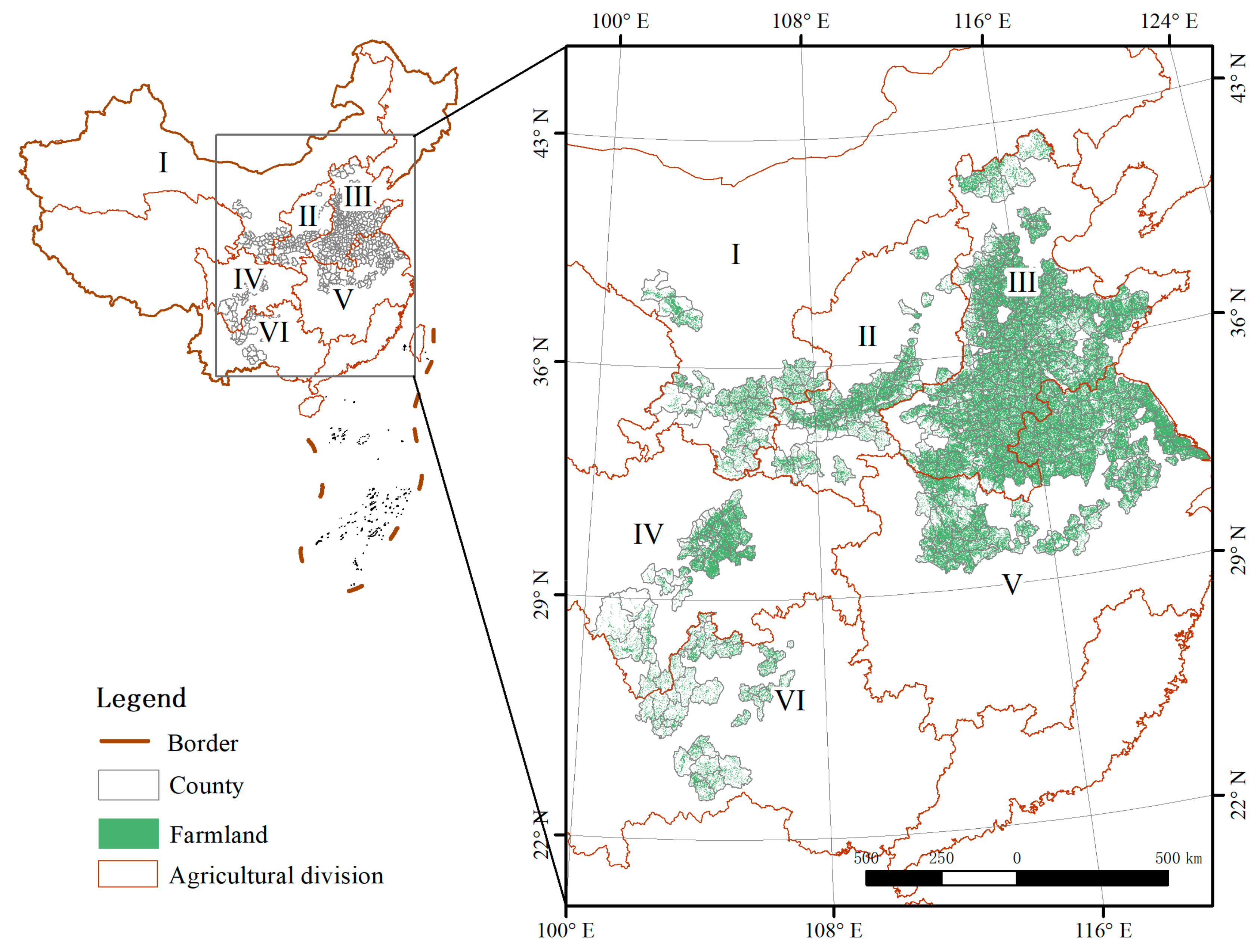
2.1. Study Area
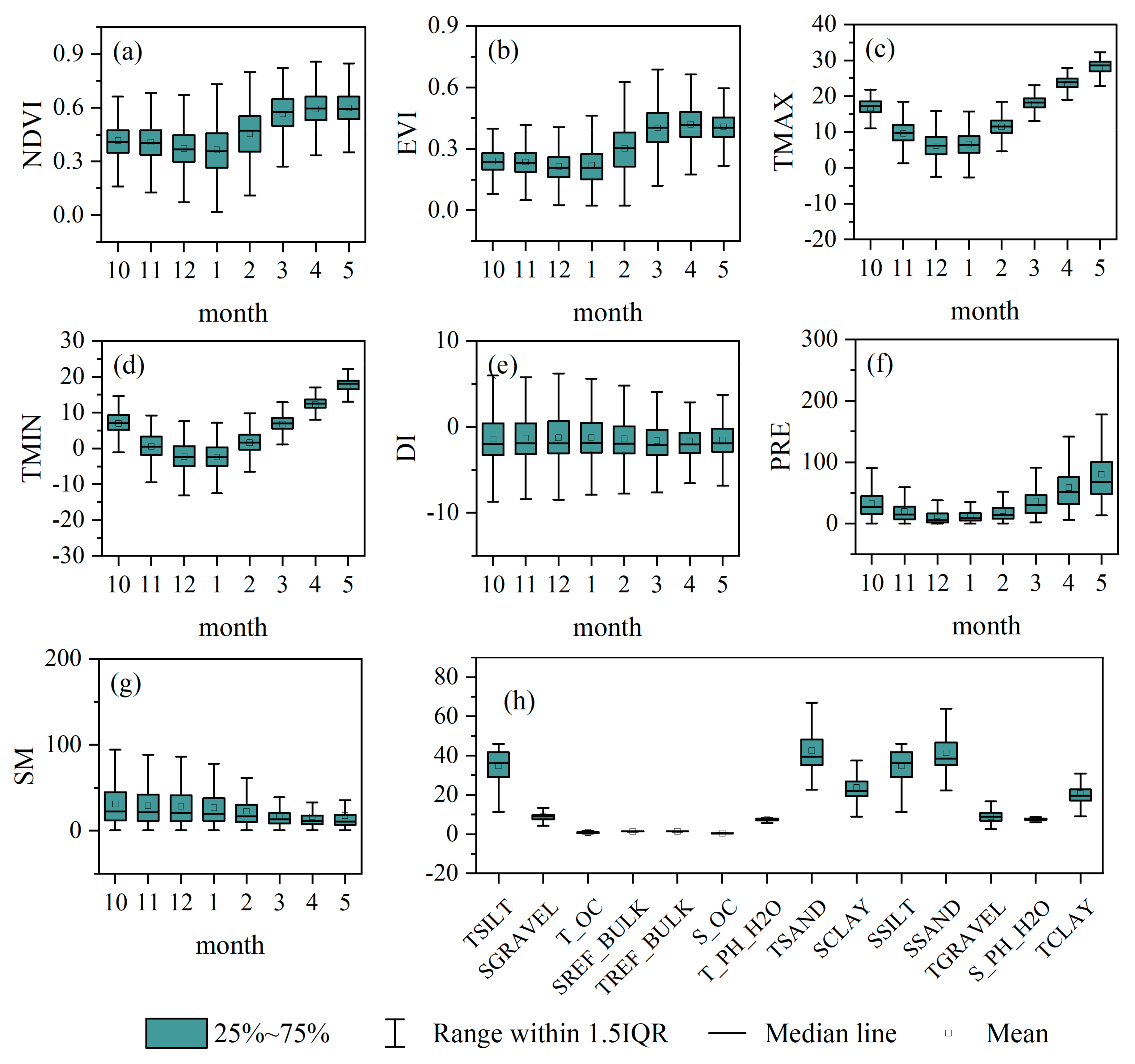
2.2. Data Sources
2.2.1. Remote Sensing Data
2.2.2. Climate Data
2.2.3. Soil Data
2.2.4. Wheat Yield Data and Planting Area
2.3. Identify the Better Time Window for the Training Settings of Wheat
2.4. Machine-Learning Methods for Estimating Crop Yield
2.4.1. K-Nearest Neighbor Regression
2.4.2. Neural Network (NN)
2.4.3. Decision Tree (DT)
2.4.4. Support Vector Machine (SVM)
2.4.5. Gaussian Process Regression (GPR)
2.4.6. Random Forest (RF)
2.4.7. Ensembles of Learning Machines
2.5. Model Evaluation
3. Results
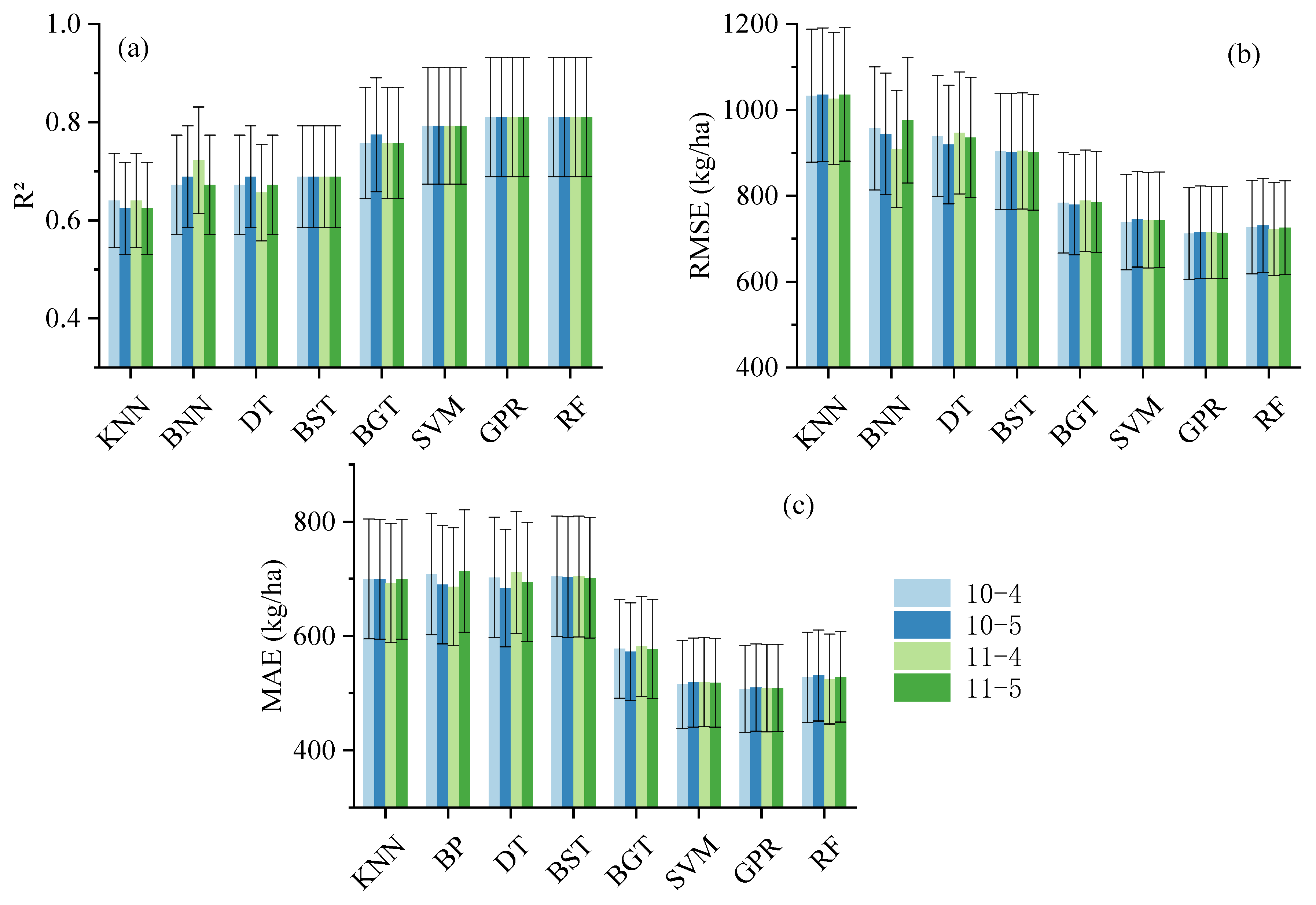
3.1. Comparison of Training Accuracy of Winter Wheat Yield Prediction Models in Different Time Windows
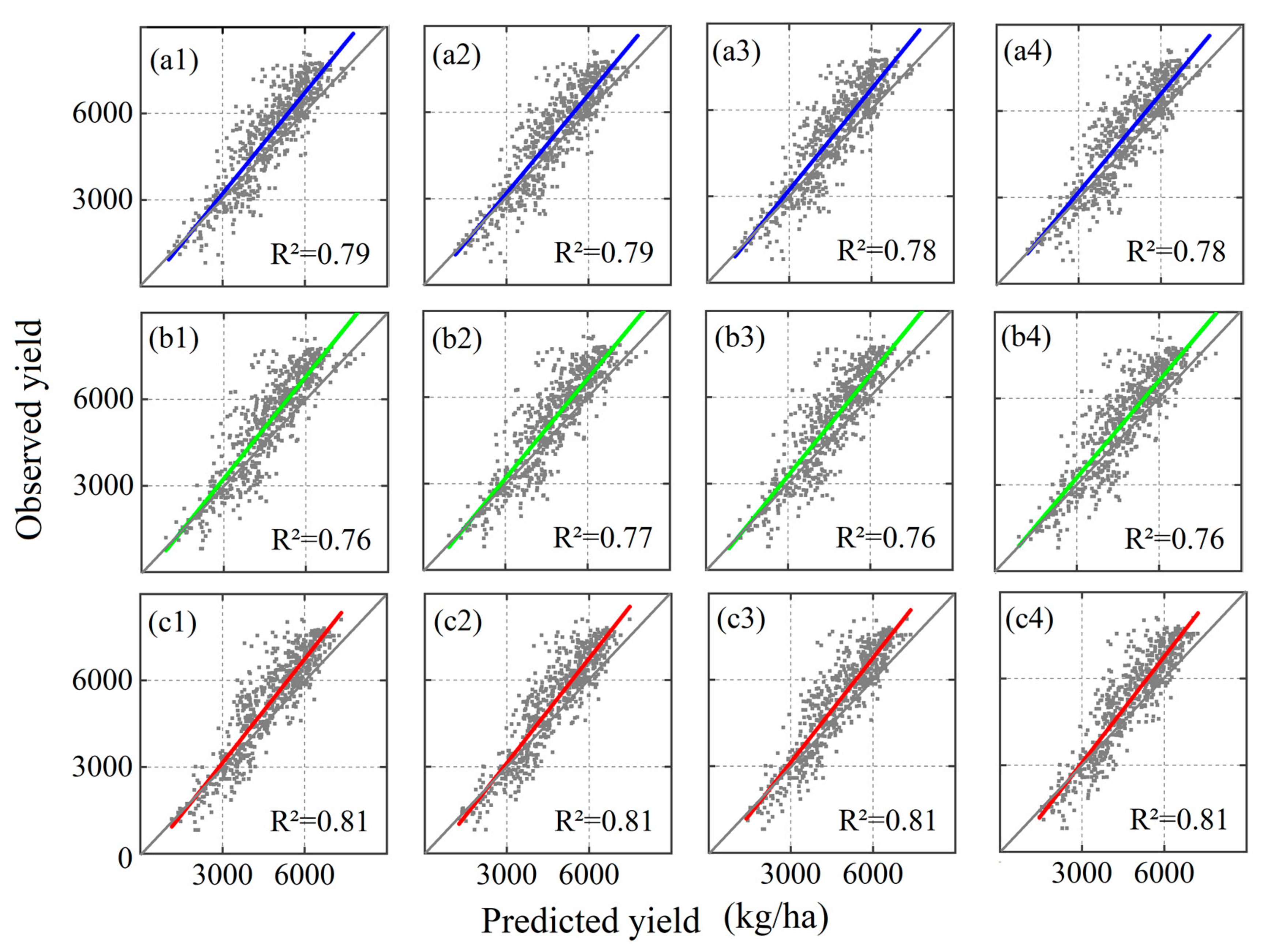
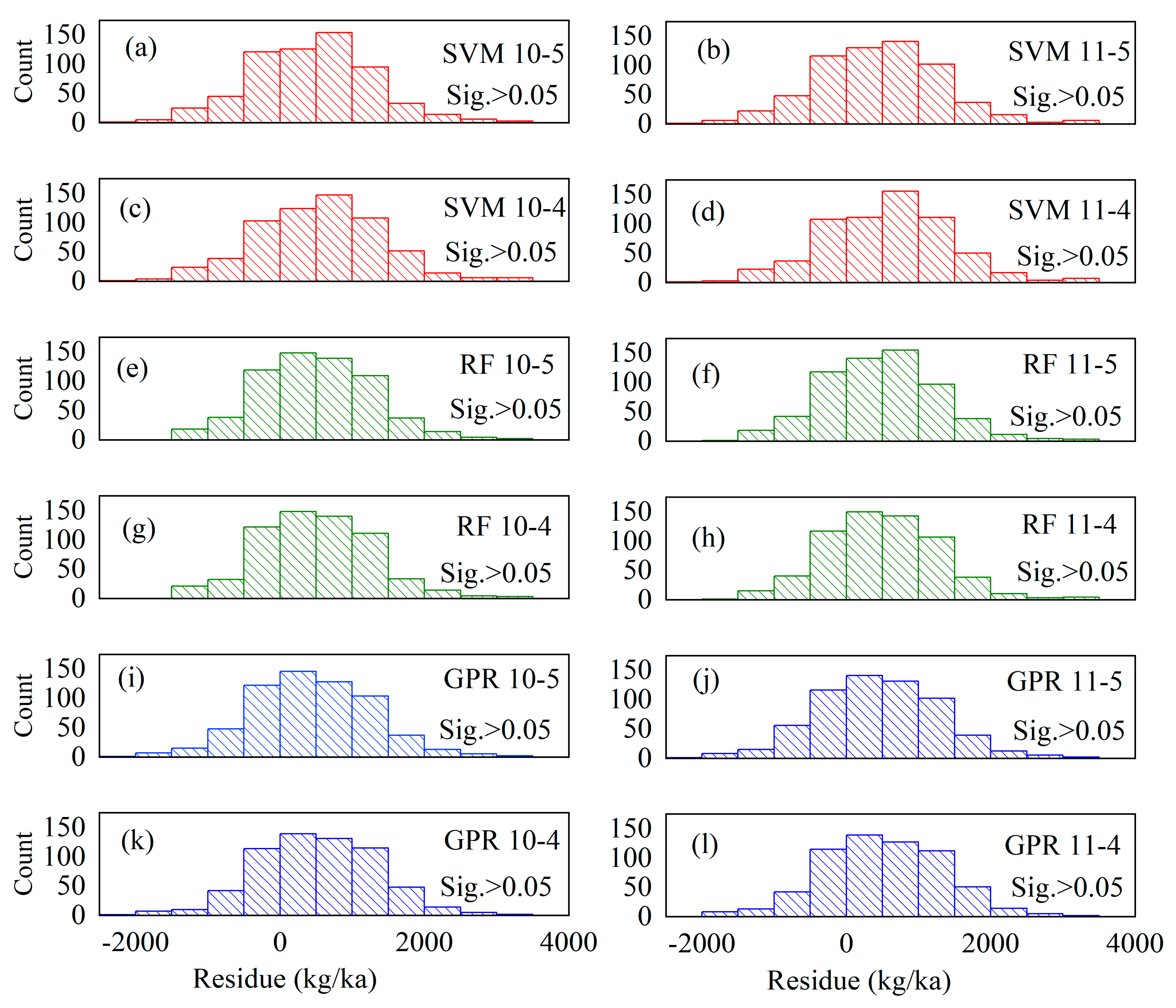
3.2. Winter Wheat Yield Predictions
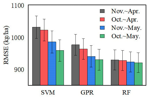
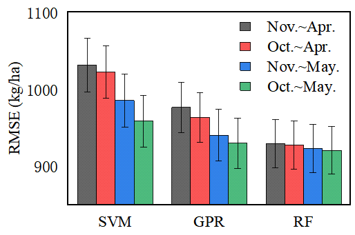
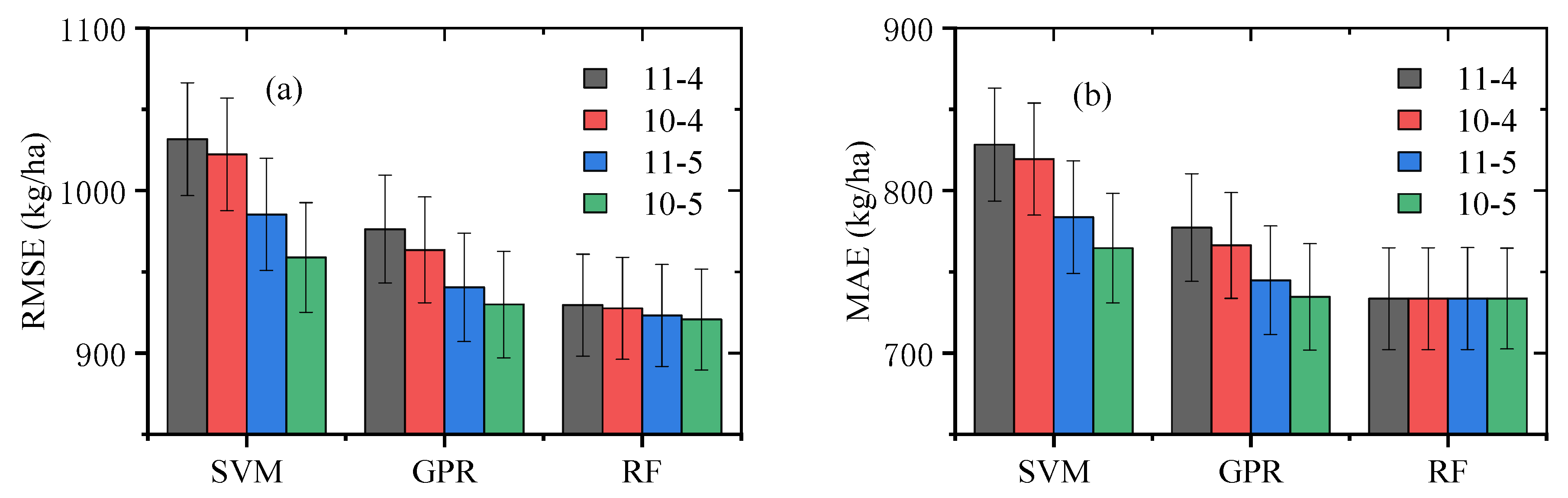
3.3. Impacts of Selecting Time Windows on Prediction Accuracy
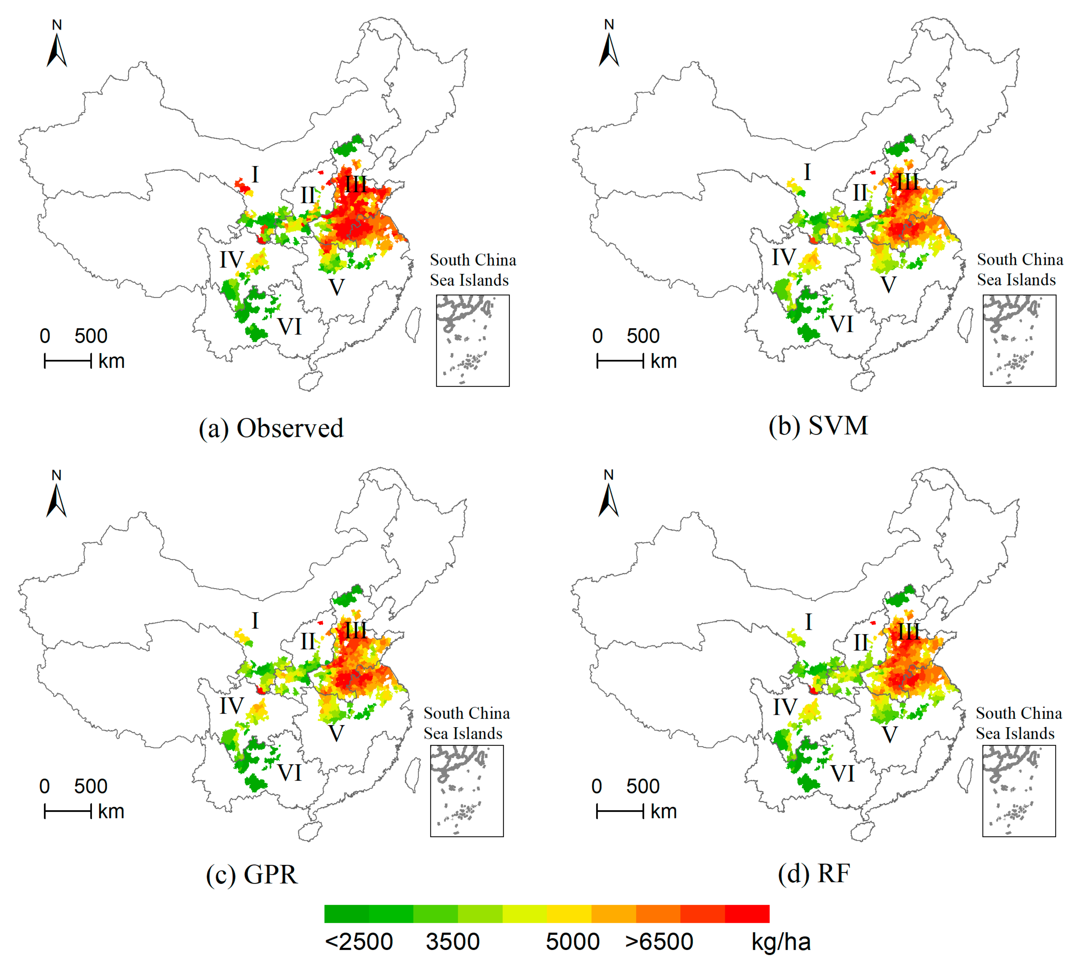
3.4. Spatial Patterns of Winter Wheat Yield Predicted
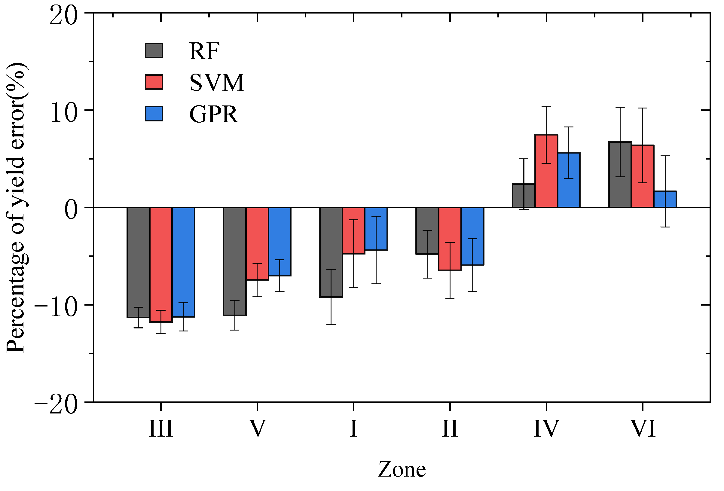
3.5. Comparison of Forecast Errors in Different Areas
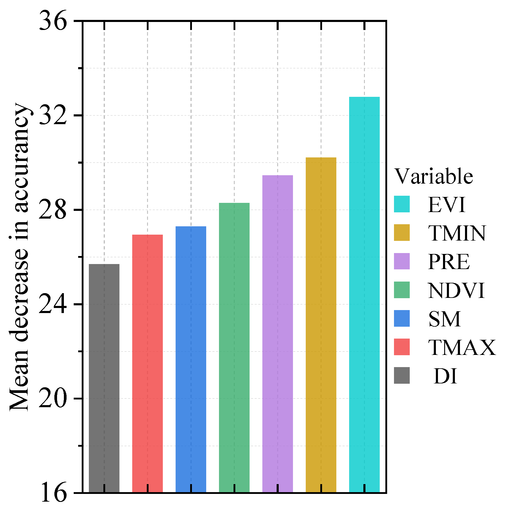
3.6. Prediction Variables and the Order of Relative Importance
4. Discussion
4.1. Model Performance for Estimating Yields in Different Time Windows
4.2. Model Performance for Regional Differences
4.3. Feature Importance in Yield Estimations
4.4. Uncertainties in the Study
5. Conclusions
Author Contributions
Funding
Conflicts of Interest
Appendix A

| Data Type | Variable | Data Description | Period | Resolution | Reference |
|---|---|---|---|---|---|
| Yield | - | Yield monitor data(kg/ha) | Year | Regional | [53] |
| Cultivated land pixel | - | Winter wheat maps | Year | 1 km * 1 km | [55] |
| Remote sensing data | NDVI | MOD13Q1 | 16-day | 250 m * 250 m | NASA LP DAAC |
| EVI | MOD13Q1 | 16-day | 250 m * 250 m | ||
| Meteorological data | TMAX | unit: % °C. | Monthly | 1/24°, ~4 km | [48] |
| TMIN | unit: % °C. | Monthly | 1/24°, ~4 km | ||
| DI | - | Monthly | 1/24°, ~4 km | ||
| PRE | unit: % mm. | Monthly | 1/24°, ~4 km | ||
| Soil data | SM | unit: % mm. | Monthly | 1/24°, ~4 km | [52] |
| T_SILT | unit: % wt. | - | 1 km | ||
| S_SILT | unit: % wt. | - | 1 km | ||
| T_GRAVEL | unit: % vol. | - | 1 km | ||
| S_GRAVEL | unit: % vol. | - | 1 km | ||
| T_OC | unit: % weight. | - | 1 km | ||
| S_OC | unit: % weight. | - | 1 km | ||
| T_REF_BULK | unit: %kg/dm3. | - | 1 km | ||
| S_REF_BULK | unit: %kg/dm3. | - | 1 km | ||
| T_PH_H2O | unit: %-log(H+). | - | 1 km | ||
| S_PH_H2O | unit: %-log(H+). | - | 1 km | ||
| T_SAND | unit: % wt. | - | 1 km | ||
| S_SAND | unit: % wt. | - | 1 km | ||
| T_CLAY | unit: % wt. | - | 1 km | ||
| S_CLAY | unit: % wt. | - | 1 km |
Appendix B

References
- Curtis, T.; Halford, N.G. Food security: The challenge of increasing wheat yield and the importance of not compromising food safety. Ann. Appl. Biol. 2014, 164, 354–372. [Google Scholar] [CrossRef] [PubMed]
- Cai, Y.; Guan, K.; Lobell, D.; Potgieter, A.B.; Wang, S.; Peng, J.; Xu, T.; Asseng, S.; Zhang, Y.; You, L.; et al. Integrating satellite and climate data to predict wheat yield in Australia using machine learning approaches. Agric. For. Meteorol. 2019, 274, 144–159. [Google Scholar] [CrossRef]
- Balaghi, R.; Tychon, B.; Eerens, H.; Jlibene, M. Empirical regression models using NDVI, rainfall and temperature data for the early prediction of wheat grain yields in Morocco. Int. J. Appl. Earth Obs. Geoinf. 2008, 10, 438–452. [Google Scholar] [CrossRef]
- Farrell, M.; Macdonald, L.M.; Butler, G.; Chirino-Valle, I.; Condron, L.M. Biochar and fertiliser applications influence phosphorus fractionation and wheat yield. Biol. Fertil. Soil. 2014, 50, 169–178. [Google Scholar] [CrossRef]
- He, Z.; Xia, X.; Zhang, Y. Breeding noodle wheat in China. In Asian Noodles: Science, Technology, and Processing; Wiley: Hoboken, NJ, USA, 2010; pp. 1–23. [Google Scholar]
- Huang, J.; Tian, L.; Liang, S.; Ma, H.; Becker-Reshef, I.; Huang, Y.; Su, W.; Zhang, X.; Zhu, D.; Wu, W. Improving winter wheat yield estimation by assimilation of the leaf area index from Landsat TM and MODIS data into the WOFOST model. Agric. For. Meteorol. 2015, 204, 106–121. [Google Scholar] [CrossRef]
- Lobell, D.B.; Burke, M.B. On the use of statistical models to predict crop yield responses to climate change. Agric. For. Meteorol. 2010, 150, 1443–1452. [Google Scholar] [CrossRef]
- Tao, F.; Yokozawa, M.; Zhang, Z. Modelling the impacts of weather and climate variability on crop productivity over a large area: A new process-based model development, optimization, and uncertainties analysis. Agric. For. Meteorol. 2009, 149, 831–850. [Google Scholar] [CrossRef]
- Tao, F.; Yokozawa, M.; Liu, J.; Zhang, Z. Climate-crop yield relationships at provincial scales in China and the impacts of recent climate trends. Clim. Res. 2008, 38, 83–94. [Google Scholar] [CrossRef]
- Lobell, D.B.; Schlenker, W.; Costa-Roberts, J. Climate trends and global crop production since 1980. Science 2011, 333, 616–620. [Google Scholar] [CrossRef]
- Shi, W.; Tao, F.; Zhang, Z. A review on statistical models for identifying climate contributions to crop yields. J. Geogr. Sci. 2013, 23, 567–576. [Google Scholar] [CrossRef]
- Tao, F.; Zhang, Z.; Shi, W.; Liu, Y.; Xiao, D.; Zhang, S.; Zhu, Z.; Wang, M.; Liu, F. Single rice growth period was prolonged by cultivars shifts, but yield was damaged by climate change during 1981–2009 in China, and late rice was just opposite. Glob. Chang. Biol. 2013, 19, 3200–3209. [Google Scholar] [CrossRef] [PubMed]
- Zhang, Z.; Song, X.; Tao, F.; Zhang, S.; Shi, W. Climate trends and crop production in China at county scale, 1980 to 2008. Theor. Appl. Climatol. 2016, 123, 291–302. [Google Scholar] [CrossRef]
- Filippi, P.; Jones, E.J.; Wimalathunge, N.S.; Somarathna, P.D.S.N.; Pozza, L.E.; Ugbaje, S.U.; Jephcott, T.G.; Paterson, S.E.; Whelan, B.M.; Bishop, T.F.A. An approach to forecast grain crop yield using multi-layered, multi-farm data sets and machine learning. Precis. Agric. 2019, 20, 1015–1029. [Google Scholar] [CrossRef]
- Jones, J.W.; Hoogenboom, G.; Porter, C.H.; Boote, K.J.; Batchelor, W.D.; Hunt, L.A.; Wilkens, P.W.; Singh, U.; Gijsman, A.J.; Ritchie, J.T. The DSSAT cropping system model. Eur. J. Agron. 2003, 18, 235–265. [Google Scholar] [CrossRef]
- Keating, B.A.; Carberry, P.S.; Hammer, G.L.; Probert, M.E.; Robertson, M.J.; Holzworth, D.; Huth, N.I.; Hargreaves, J.N.; Meinke, H.; Hochman, Z.; et al. An overview of APSIM, a model designed for farming systems simulation. Eur. J. Agron. 2003, 18, 267–288. [Google Scholar] [CrossRef]
- Tao, F.; Zhang, Z.; Liu, J.; Yokozawa, M. Modelling the impacts of weather and climate variability on crop productivity over a large area: A new super-ensemble-based probabilistic projection. Agric. For. Meteorol. 2009, 149, 1266–1278. [Google Scholar] [CrossRef]
- Van Diepen, C.V.; Wolf, J.; Van Keulen, H.; Rappoldt, C. WOFOST: A simulation model of crop production. Soil Use Manag. 1989, 5, 16–24. [Google Scholar] [CrossRef]
- Lobell, D.B. The use of satellite data for crop yield gap analysis. Field Crop. Res. 2013, 143, 56–64. [Google Scholar] [CrossRef]
- Aghighi, H.; Azadbakht, M.; Ashourloo, D.; Shahrabi, H.S.; Radiom, S. Machine Learning Regression Techniques for the Silage Maize Yield Prediction Using Time-Series Images of Landsat 8 OLI. IEEE J. Sel. Top. App. Earth Obs. Remote Sens. 2018, 11, 4563–4577. [Google Scholar] [CrossRef]
- Stas, M.; Van Orshoven, J.; Dong, Q.; Heremans, S.; Zhang, B. A comparison of machine learning algorithms for regional wheat yield prediction using NDVI time series of SPOT-VGT. In Proceedings of the 2016 Fifth International Conference on Agro-Geoinformatics (Agro-Geoinformatics), Tianjin, China, 18–20 July 2016; pp. 1–5. [Google Scholar]
- Saeed, U.; Dempewolf, J.; Becker-Reshef, I.; Khan, A.; Ahmad, A.; Wajid, S.A. Forecasting wheat yield from weather data and MODIS NDVI using Random Forests for Punjab province, Pakistan. Int. J. Remote Sens. 2017, 38, 4831–4854. [Google Scholar] [CrossRef]
- Johnson, M.D.; Hsieh, W.W.; Cannon, A.J.; Davidson, A.; Bédard, F. Crop yield forecasting on the Canadian Prairies by remotely sensed vegetation indices and machine learning methods. Agric. For. Meteorol. 2016, 218–219, 74–84. [Google Scholar] [CrossRef]
- Satir, O.; Berberoglu, S. Crop yield prediction under soil salinity using satellite derived vegetation indices. Field Crop. Res. 2016, 192, 134–143. [Google Scholar] [CrossRef]
- Witten, I.H.; Frank, E.; Hall, M.A.; Pal, C.J. Data Mining: Practical Machine Learning Tools and Techniques; Morgan Kaufmann: Burlington, MA, USA, 2016. [Google Scholar]
- Cai, Y.; Guan, K.; Peng, J.; Wang, S.; Seifert, C.; Wardlow, B.; Li, Z. A high-performance and in-season classification system of field-level crop types using time-series Landsat data and a machine learning approach. Remote Sens. Environ. 2018, 210, 35–47. [Google Scholar] [CrossRef]
- Crane-Droesch, A. Machine learning methods for crop yield prediction and climate change impact assessment in agriculture. Environ. Res. Lett. 2018, 13, 114003. [Google Scholar] [CrossRef]
- Iqbal, M.A.; Shen, Y.; Stricevic, R.; Pei, H.; Sun, H.; Amiri, E.; Penas, A.; Del Rio, S. Evaluation of the FAO AquaCrop model for winter wheat on the North China Plain under deficit irrigation from field experiment to regional yield simulation. Agric. Water Manag. 2014, 135, 61–72. [Google Scholar] [CrossRef]
- Chen, Y.; Zhang, Z.; Tao, F. Improving regional winter wheat yield estimation through assimilation of phenology and leaf area index from remote sensing data. Eur. J. Agron. 2018, 101, 163–173. [Google Scholar] [CrossRef]
- Russello, H. Convolutional Neural Networks for Crop Yield Prediction Using Satellite Images. Master’s Thesis, University of Amsterdam, Amsterdam, The Netherlands, 2018. [Google Scholar]
- Ren, J.; Chen, Z.; Zhou, Q.; Tang, H. Regional yield estimation for winter wheat with MODIS-NDVI data in Shandong, China. Int. J. Appl. Earth Obs. Geoinf. 2008, 10, 403–413. [Google Scholar] [CrossRef]
- Mo, X.; Liu, S.; Lin, Z.; Xu, Y.; Xiang, Y.; McVicar, T.R. Prediction of crop yield, water consumption and water use efficiency with a SVAT-crop growth model using remotely sensed data on the North China Plain. Ecol. Model. 2005, 183, 301–322. [Google Scholar] [CrossRef]
- Lv, Z.; Liu, X.; Cao, W.; Zhu, Y. Climate change impacts on regional winter wheat production in main wheat production regions of China. Agric. For. Meteorol. 2013, 171, 234–248. [Google Scholar] [CrossRef]
- Xiao, G.; Zhang, Q.; Yao, Y.; Zhao, H.; Wang, R.; Bai, H.; Zhang, F. Impact of recent climatic change on the yield of winter wheat at low and high altitudes in semi-arid northwestern China. Agric. Ecosyst. Environ. 2008, 127, 37–42. [Google Scholar] [CrossRef]
- Tao, F.; Xiao, D.; Zhang, S.; Zhang, Z.; Rötter, R.P. Wheat yield benefited from increases in minimum temperature in the Huang-Huai-Hai Plain of China in the past three decades. Agric. For. Meteorol. 2017, 239, 1–14. [Google Scholar] [CrossRef]
- Tao, F.; Zhang, Z.; Zhang, S.; Rötter, R.P. Heat stress impacts on wheat growth and yield were reduced in the Huang-Huai-Hai Plain of China in the past three decades. Eur. J. Agron. 2015, 71, 44–52. [Google Scholar] [CrossRef]
- Gandhi, N.; Armstrong, L.J.; Petkar, O.; Tripathy, A.K. Rice crop yield prediction in India using support vector machines. In Proceedings of the 2016 13th International Joint Conference on Computer Science and Software Engineering (JCSSE 2016), Khon Kaen, Thailand, 13–15 July 2016; pp. 1–5. [Google Scholar]
- Gorelick, N.; Hancher, M.; Dixon, M.; Ilyushchenko, S.; Thau, D.; Moore, R. Google Earth Engine: Planetary-scale geospatial analysis for everyone. Remote Sens. Environ. 2017, 202, 18–27. [Google Scholar] [CrossRef]
- Mutanga, O.; Kumar, L. Google Earth Engine Applications. Remote Sens. 2019, 11, 591. [Google Scholar] [CrossRef]
- Jin, Z.; Azzari, G.; You, C.; Di Tommaso, S.; Aston, S.; Burke, M.; Lobell, D.B. Smallholder maize area and yield mapping at national scales with Google Earth Engine. Remote Sens. Environ. 2019, 228, 115–128. [Google Scholar] [CrossRef]
- Huang, J.; Wang, H.; Dai, Q.; Han, D. Analysis of NDVI data for crop identification and yield estimation. IEEE J. Stars. 2014, 7, 4374–4384. [Google Scholar] [CrossRef]
- Mkhabela, M.S.; Bullock, P.; Raj, S.; Wang, S.; Yang, Y. Crop yield forecasting on the Canadian Prairies using MODIS NDVI data. Agric. For. Meteorol. 2011, 151, 385–393. [Google Scholar] [CrossRef]
- Feng, P.; Wang, B.; Liu, D.L.; Xing, H.; Ji, F.; Macadam, I.; Ruan, H.; Yu, Q. Impacts of rainfall extremes on wheat yield in semi-arid cropping systems in eastern Australia. Clim. Chang. 2018, 147, 555–569. [Google Scholar] [CrossRef]
- Zhang, Z.; Chen, Y.; Wang, C.; Wang, P.; Tao, F. Future extreme temperature and its impact on rice yield in China. Int. J. Climatol. 2017, 37, 4814–4827. [Google Scholar] [CrossRef]
- Challinor, A.J.; Watson, J.; Lobell, D.B.; Howden, S.M.; Smith, D.R.; Chhetri, N. A meta-analysis of crop yield under climate change and adaptation. Nat. Clim. Chang. 2014, 4, 287–291. [Google Scholar] [CrossRef]
- Webber, H.; Ewert, F.; Olesen, J.E.; Müller, C.; Fronzek, S.; Ruane, A.C.; Bourgault, M.; Martre, P.; Ababaei, B.; Bindi, M.; et al. Diverging importance of drought stress for maize and winter wheat in Europe. Nat. Commun. 2018, 9, 4249. [Google Scholar] [CrossRef] [PubMed]
- Ummenhofer, C.C.; Xu, H.; Twine, T.E.; Girvetz, E.H.; McCarthy, H.R.; Chhetri, N.; Nicholas, K.A. How Climate Change Affects Extremes in Maize and Wheat Yield in Two Cropping Regions. J. Clim. 2015, 28, 4653–4687. [Google Scholar] [CrossRef]
- Abatzoglou, J.T.; Dobrowski, S.Z.; Parks, S.A.; Hegewisch, K.C. TerraClimate, a high-resolution global dataset of monthly climate and climatic water balance from 1958–2015. Sci. Data 2018, 5, 170191. [Google Scholar] [CrossRef] [PubMed]
- Khataar, M.; Mohammadi, M.H.; Shabani, F. Soil salinity and matric potential interaction on water use, water use efficiency and yield response factor of bean and wheat. Sci. Rep. 2018, 8, 2679. [Google Scholar] [CrossRef] [PubMed]
- He, G.; Wang, Z.; Li, F.; Dai, J.; Li, Q.; Xue, C.; Cao, H.; Wang, S.; Malhi, S.S. Soil water storage and winter wheat productivity affected by soil surface management and precipitation in dryland of the Loess Plateau, China. Agric. Water Manag. 2016, 171, 1–9. [Google Scholar] [CrossRef]
- Li, H.; Xue, J.; Gao, Z.; Xue, N.; Yang, Z. Response of yield increase for dryland winter wheat to tillage practice during summer fallow and sowing method in the Loess Plateau of China. J. Integr. Agric. 2018, 17, 817–825. [Google Scholar] [CrossRef]
- Fischer, G.; Nachtergaele, F.; Prieler, S.; Van Velthuizen, H.T.; Verelst, L.; Wiberg, D. Global Agro-Ecological Zones Assessment for Agriculture (GAEZ 2008); IIASA: Laxenburg, Austria; FAO: Rome, Italy, 2008. [Google Scholar]
- Tao, F.; Zhang, Z.; Zhang, S.; Zhu, Z.; Shi, W. Response of crop yields to climate trends since 1980 in China. Clim. Res. 2012, 54, 233–247. [Google Scholar] [CrossRef]
- Chen, Y.; Zhang, Z.; Tao, F.; Wang, P.; Wei, X. Spatio-temporal patterns of winter wheat yield potential and yield gap during the past three decades in North China. Field Crop. Res. 2017, 206, 11–20. [Google Scholar] [CrossRef]
- Luo, Y.; Zhang, Z.; Chen, Y.; Li, Z.; Tao, F. ChinaCropPhen1km: A high-resolution crop phenological dataset for three staple crops in China during 2000–2015 based on LAI products. Earth Syst. Sci. Data Discuss. 2019, 2019. [Google Scholar] [CrossRef]
- Sakamoto, T.; Yokozawa, M.; Toritani, H.; Shibayama, M.; Ishitsuka, N.; Ohno, H. A crop phenology detection method using time-series MODIS data. Remote Sens. Environ. 2005, 96, 366–374. [Google Scholar] [CrossRef]
- Appelhans, T.; Mwangomo, E.; Hardy, D.R.; Hemp, A.; Nauss, T. Evaluating machine learning approaches for the interpolation of monthly air temperature at Mt. Kilimanjaro, Tanzania. Spat. Stat. 2015, 14, 91–113. [Google Scholar] [CrossRef]
- Aha, D.W.; Kibler, D.; Albert, M.K. Instance-based learning algorithms. Mach. Learn. 1991, 6, 37–66. [Google Scholar] [CrossRef]
- Wang, B.; Gu, X.; Ma, L.; Yan, S. Temperature error correction based on BP neural network in meteorological wireless sensor network. In Proceedings of the International Conference on Cloud Computing and Security, Nanjing, China, 29–31 July 2016; Springer: Cham, Switzerland, 2016; pp. 117–132. [Google Scholar]
- Bélisle, E.; Huang, Z.; Le Digabel, S.; Gheribi, A.E. Evaluation of machine learning interpolation techniques for prediction of physical properties. Comput. Mater. Sci. 2015, 98, 170–177. [Google Scholar] [CrossRef]
- Xu, M.; Watanachaturaporn, P.; Varshney, P.; Arora, M. Decision tree regression for soft classification of remote sensing data. Remote Sens. Environ. 2005, 97, 322–336. [Google Scholar] [CrossRef]
- Song, Y.Y.; Lu, Y. Decision tree methods: Applications for classification and prediction. Shanghai Arch. Psychiatry 2015, 27, 130–135. [Google Scholar] [PubMed]
- Polat, K.; Güneş, S. A novel hybrid intelligent method based on C4.5 decision tree classifier and one-against-all approach for multi-class classification problems. Expert Syst. Appl. 2009, 36, 1587–1592. [Google Scholar] [CrossRef]
- Gunn, S.R. Support vector machines for classification and regression. ISIS Tech. Rep. 1998, 14, 5–16. [Google Scholar]
- Hearst, M.A.; Dumais, S.T.; Osuna, E.; Platt, J.; Scholkopf, B. Support vector machines. IEEE Intell. Syst. Appl. 1998, 13, 18–28. [Google Scholar] [CrossRef]
- Rasmussen, C.E. Gaussian processes in machine learning. In Summer School on Machine Learning; Springer: Cambridge, MA, USA, 2003; pp. 63–71. [Google Scholar]
- Williams, C.K.; Rasmussen, C.E. Gaussian Processes for Machine Learning; MIT Press: Cambridge, MA, USA, 2006. [Google Scholar]
- Breiman, L. Random forests. Mach. Learn. 2001, 45, 5–32. [Google Scholar] [CrossRef]
- Rhee, J.; Im, J. Meteorological drought forecasting for ungauged areas based on machine learning: Using long-range climate forecast and remote sensing data. Agric. For. Meteorol. 2017, 237–238, 105–122. [Google Scholar] [CrossRef]
- Vincenzi, S.; Zucchetta, M.; Franzoi, P.; Pellizzato, M.; Pranovi, F.; De Leo, G.A.; Torricelli, P. Application of a Random Forest algorithm to predict spatial distribution of the potential yield of Ruditapes philippinarum in the Venice lagoon, Italy. Ecol. Model. 2011, 222, 1471–1478. [Google Scholar] [CrossRef]
- Strobl, C.; Boulesteix, A.L.; Zeileis, A.; Hothorn, T. Bias in random forest variable importance measures: Illustrations, sources and a solution. BMC Bioinform. 2007, 8, 25. [Google Scholar] [CrossRef]
- Dietterich, T.G. Ensemble Methods in Machine Learning. In Proceedings of the International Workshop on Multiple Classifier Systems, Cagliari, Italy, 21–23 June 2000; Springer: Berlin/Heidelberg, Germany, 2000; pp. 1–15. [Google Scholar]
- Voyant, C.; Notton, G.; Kalogirou, S.; Nivet, M.; Paoli, C.; Motte, F.; Fouilloy, A. Machine learning methods for solar radiation forecasting: A review. Renew. Energy 2017, 105, 569–582. [Google Scholar] [CrossRef]
- Quinlan, J.R. Bagging, Boosting, and C4. 5. In Proceedings of the Thirteenth National Conference on Artificial Intelligence, Portland, OR, USA, 4—8 August 1996; Volume 1, pp. 725–730. [Google Scholar]
- Arlot, S.; Celisse, A. A survey of cross-validation procedures for model selection. Stat. Surv. 2010, 4, 40–79. [Google Scholar] [CrossRef]
- Picard, R.R.; Cook, R.D. Cross-validation of regression models. J. Am. Stat. Assoc. 1984, 79, 575–583. [Google Scholar] [CrossRef]
- Johnson, D.M. An assessment of pre- and within-season remotely sensed variables for forecasting corn and soybean yields in the United States. Remote Sens. Environ. 2014, 141, 116–128. [Google Scholar] [CrossRef]
- Labus, M.P.; Nielsen, G.A.; Lawrence, R.L.; Engel, R.; Long, D.S. Wheat yield estimates using multi-temporal NDVI satellite imagery. Int. J. Remote Sens. 2002, 23, 4169–4180. [Google Scholar] [CrossRef]
- Doraiswamy, P.C.; Cook, P.W. Spring wheat yield assessment using NOAA AVHRR data. Can. J. Remote Sens. 1995, 21, 43–51. [Google Scholar] [CrossRef]
- Tsimba, R.; Edmeades, G.O.; Millner, J.P.; Kemp, P.D. The effect of planting date on maize grain yields and yield components. Field Crop. Res. 2013, 150, 135–144. [Google Scholar] [CrossRef]
- Tsimba, R.; Edmeades, G.O.; Millner, J.P.; Kemp, P.D. The effect of planting date on maize: Phenology, thermal time durations and growth rates in a cool temperate climate. Field Crop. Res. 2013, 150, 145–155. [Google Scholar] [CrossRef]
- Bolton, D.K.; Friedl, M.A. Forecasting crop yield using remotely sensed vegetation indices and crop phenology metrics. Agric. For. Meteorol. 2013, 173, 74–84. [Google Scholar] [CrossRef]
- Jeong, J.H.; Resop, J.P.; Mueller, N.D.; Fleisher, D.H.; Yun, K.; Butler, E.E.; Timlin, D.J.; Shim, K.; Gerber, J.S.; Reddy, V.R.; et al. Random Forests for Global and Regional Crop Yield Predictions. PLoS ONE 2016, 11, e156571. [Google Scholar] [CrossRef] [PubMed]
- Kim, N.; Lee, Y. Machine Learning Approaches to Corn Yield Estimation Using Satellite Images and Climate Data: A Case of Iowa State. J. Korean Soc. Surv. Geod. Photogramm. Cartogr. 2016, 34, 383–390. [Google Scholar] [CrossRef]
- Zhao, Y.; Lobell, D.B. Assessing the heterogeneity and persistence of farmers’ maize yield performance across the North China Plain. Field Crop. Res. 2017, 205, 55–66. [Google Scholar] [CrossRef]
- Ji, B.; Sun, Y.; Yang, S.; Wan, J. Artificial neural networks for rice yield prediction in mountainous regions. J. Agric. Sci. 2007, 145, 249. [Google Scholar] [CrossRef]
- Lai, Y.R.; Pringle, M.J.; Kopittke, P.M.; Menzies, N.W.; Orton, T.G.; Dang, Y.P. An empirical model for prediction of wheat yield, using time-integrated Landsat NDVI. Int. J. Appl. Earth Obs. 2018, 72, 99–108. [Google Scholar] [CrossRef]
- Son, N.T.; Chen, C.F.; Chen, C.R.; Minh, V.Q.; Trung, N.H. A comparative analysis of multitemporal MODIS EVI and NDVI data for large-scale rice yield estimation. Agric. For. Meteorol. 2014, 197, 52–64. [Google Scholar] [CrossRef]
- Shanahan, J.F.; Schepers, J.S.; Francis, D.D.; Varvel, G.E.; Wilhelm, W.W.; Tringe, J.M.; Schlemmer, M.R.; Major, D.J. Use of remote-sensing imagery to estimate corn grain yield. Agron. J. 2001, 93, 583–589. [Google Scholar] [CrossRef]
- Fontana, D.C.; Potgieter, A.B.; Apan, A. Assessing the relationship between shire winter crop yield and seasonal variability of the MODIS NDVI and EVI images. Appl. GIS 2007, 3, 1–16. [Google Scholar]
- Hatfield, J.L. Remote sensing estimators of potential and actual crop yield. Remote Sens. Environ. 1983, 13, 301–311. [Google Scholar] [CrossRef]
- Chen, Y.; Zhang, Z.; Tao, F.; Palosuo, T.; Rötter, R.P. Impacts of heat stress on leaf area index and growth duration of winter wheat in the North China Plain. Field Crop. Res. 2018, 222, 230–237. [Google Scholar] [CrossRef]
- Slafer, G.A.; Savin, R. Developmental Base Temperature in Different Phenological Phases of Wheat (Triticum aestivum). J. Exp. Bot. 1991, 42, 1077–1082. [Google Scholar] [CrossRef]
- Garg, D.; Sareen, S.; Dalal, S.; Tiwari, R.; Singh, R. Grain filling duration and temperature pattern influence on the performance of wheat genotypes under late planting. Cereal Res. Commun. 2013, 41, 500–507. [Google Scholar] [CrossRef]
- Lobell, D.B.; Sibley, A.; Ivan Ortiz-Monasterio, J. Extreme heat effects on wheat senescence in India. Nat. Clim. Chang. 2012, 2, 186–189. [Google Scholar] [CrossRef]
- Biscoe, P.V.; Gallagher, J.N. Weather, Dry Matter Production and Yield. In Proceedings of the Environmental Effects on Crop Physiology, a Symposium Held at Long Ashton Research Station, University of Bristol, Bristol, UK, 13–16 April 1975; Academic Press: New York, NY, USA, 1977. [Google Scholar]
- Semenov, M.A.; Shewry, P.R. Modelling predicts that heat stress, not drought, will increase vulnerability of wheat in Europe. Sci. Rep. 2011, 1, 66. [Google Scholar] [CrossRef]
- Kern, A.; Barcza, Z.; Marjanović, H.; Árendás, T.; Fodor, N.; Bónis, P.; Bognár, P.; Lichtenberger, J. Statistical modelling of crop yield in Central Europe using climate data and remote sensing vegetation indices. Agric. For. Meteorol. 2018, 260–261, 300–320. [Google Scholar] [CrossRef]
- Webber, H.; Ewert, F.; Kimball, B.A.; Siebert, S.; White, J.W.; Wall, G.W.; Ottman, M.J.; Trawally, D.; Gaiser, T. Simulating canopy temperature for modelling heat stress in cereals. Environ. Model. Softw. 2016, 77, 143–155. [Google Scholar] [CrossRef]
- Siebert, S.; Webber, H.; Rezaei, E.E. Weather impacts on crop yields-searching for simple answers to a complex problem. Environ. Res. Lett. 2017, 12, 81001. [Google Scholar] [CrossRef]
- Porter, J.R.; Gawith, M. Temperatures and the growth and development of wheat: A review. Eur. J. Agron. 1999, 10, 23–36. [Google Scholar] [CrossRef]
- Zhao, H.; Dai, T.; Jing, Q.; Jiang, D.; Cao, W. Leaf senescence and grain filling affected by post-anthesis high temperatures in two different wheat cultivars. Plant Growth Regul. 2007, 51, 149–158. [Google Scholar] [CrossRef]
- Eitzinger, J.; Štastná, M.; Žalud, Z.; Dubrovský, M. A simulation study of the effect of soil water balance and water stress on winter wheat production under different climate change scenarios. Agric. Water Manag. 2003, 61, 195–217. [Google Scholar] [CrossRef]
- Carew, R.; Smith, E.G.; Grant, C. Factors Influencing Wheat Yield and Variability: Evidence from Manitoba, Canada. J. Agric. Appl. Econ. 2009, 41, 625–639. [Google Scholar] [CrossRef]
- Siebert, S.; Ewert, F. Future crop production threatened by extreme heat. Environ. Res. Lett. 2014, 9, 41001. [Google Scholar] [CrossRef]
- Su, Y.; Xu, H.; Yan, L. Support vector machine-based open crop model (SBOCM): Case of rice production in China. Saudi J. Biol. Sci. 2017, 24, 537–547. [Google Scholar] [CrossRef]
- Tack, J.; Barkley, A.; Nalley, L.L. Effect of warming temperatures on US wheat yields. Proc. Natl. Acad. Sci. USA 2015, 112, 6931–6936. [Google Scholar] [CrossRef] [PubMed]
- Tao, J.; Wu, W.; Yong, Z.; Yu, W.; Jiang, Y. Mapping winter wheat using phenological feature of peak before winter on the North China Plain based on time-series MODIS data. J. Integr. Agric. 2017, 16, 348–359. [Google Scholar] [CrossRef]
- Zhou, G.; Liu, X.; Liu, M. Assimilating Remote Sensing Phenological Information into the WOFOST Model for Rice Growth Simulation. Remote Sens. 2019, 11, 268. [Google Scholar] [CrossRef]
- Sokoto, M.B.; Abubakar, I.U.; Dikko, A.U. Correlation analysis of some growth, yield, yield components and grain quality of wheat (Triticum aestivum L.). Niger. J. Basic Appl. Sci. 2012, 20, 349–356. [Google Scholar]
- Zhang, X.; Friedl, M.A.; Schaaf, C.B.; Strahler, A.H.; Hodges, J.C.; Gao, F.; Reed, B.C.; Huete, A. Monitoring vegetation phenology using MODIS. Remote Sens. Environ. 2003, 84, 471–475. [Google Scholar] [CrossRef]
- Motohka, T.; Nasahara, K.N.; Oguma, H.; Tsuchida, S. Applicability of green-red vegetation index for remote sensing of vegetation phenology. Remote Sens. 2010, 2, 2369–2387. [Google Scholar] [CrossRef]
- Mutanga, O.; Skidmore, A.K. Narrow band vegetation indices overcome the saturation problem in biomass estimation. Int. J. Remote Sens. 2004, 25, 3999–4014. [Google Scholar] [CrossRef]
- Santin-Janin, H.; Garel, M.; Chapuis, J.; Pontier, D. Assessing the performance of NDVI as a proxy for plant biomass using non-linear models: A case study on the Kerguelen archipelago. Polar Biol. 2009, 32, 861–871. [Google Scholar] [CrossRef]
- Huete, A.; Didan, K.; Miura, T.; Rodriguez, E.P.; Gao, X.; Ferreira, L.G. Overview of the radiometric and biophysical performance of the MODIS vegetation indices. Remote Sens. Environ. 2002, 83, 195–213. [Google Scholar] [CrossRef]
- Wang, C.; Lin, W. Winter wheat yield estimation based on MODIS EVI. Nongye Gongcheng Xuebao/Trans. Chin. Soc. Agric. Eng. 2005, 21, 90–94. [Google Scholar]
- Kouadio, L.; Newlands, N.; Davidson, A.; Zhang, Y.; Chipanshi, A. Assessing the Performance of MODIS NDVI and EVI for Seasonal Crop Yield Forecasting at the Ecodistrict Scale. Remote Sens. 2014, 6, 10193–10214. [Google Scholar] [CrossRef]
- Taylor, J.A.; McBratney, A.B.; Whelan, B.M. Establishing Management Classes for Broadacre Agricultural Production. Agron. J. 2007, 99, 1366–1376. [Google Scholar] [CrossRef]
- Battude, M.; Al Bitar, A.; Morin, D.; Cros, J.; Huc, M.; Sicre, C.M.; Le Dantec, V.; Demarez, V. Estimating maize biomass and yield over large areas using high spatial and temporal resolution Sentinel-2 like remote sensing data. Remote Sens. Environ. 2016, 184, 668–681. [Google Scholar] [CrossRef]
- Vergara-Díaz, O.; Zaman-Allah, M.A.; Masuka, B.; Hornero, A.; Zarco-Tejada, P.; Prasanna, B.M.; Cairns, J.E.; Araus, J.L. A novel remote sensing approach for prediction of maize yield under different conditions of nitrogen fertilization. Front. Plant Sci. 2016, 7, 666. [Google Scholar] [CrossRef]
- Jin, Z.; Azzari, G.; Burke, M.; Aston, S.; Lobell, D. Mapping Smallholder Yield Heterogeneity at Multiple Scales in Eastern Africa. Remote Sens. 2017, 9, 931. [Google Scholar] [CrossRef]
- Vereecken, H.; Weihermüller, L.; Jonard, F.; Montzka, C. Characterization of crop canopies and water stress related phenomena using microwave remote sensing methods: A review. Vadose Zone J. 2012, 11. [Google Scholar] [CrossRef]
- Murdoch, W.J.; Singh, C.; Kumbier, K.; Abbasi-Asl, R.; Yu, B. Definitions, methods, and applications in interpretable machine learning. Proc. Natl. Acad. Sci. USA 2019, 116, 22071–22080. [Google Scholar] [CrossRef] [PubMed]


© 2020 by the authors. Licensee MDPI, Basel, Switzerland. This article is an open access article distributed under the terms and conditions of the Creative Commons Attribution (CC BY) license (http://creativecommons.org/licenses/by/4.0/).
Share and Cite
Han, J.; Zhang, Z.; Cao, J.; Luo, Y.; Zhang, L.; Li, Z.; Zhang, J. Prediction of Winter Wheat Yield Based on Multi-Source Data and Machine Learning in China. Remote Sens. 2020, 12, 236. https://doi.org/10.3390/rs12020236
Han J, Zhang Z, Cao J, Luo Y, Zhang L, Li Z, Zhang J. Prediction of Winter Wheat Yield Based on Multi-Source Data and Machine Learning in China. Remote Sensing. 2020; 12(2):236. https://doi.org/10.3390/rs12020236
Chicago/Turabian StyleHan, Jichong, Zhao Zhang, Juan Cao, Yuchuan Luo, Liangliang Zhang, Ziyue Li, and Jing Zhang. 2020. "Prediction of Winter Wheat Yield Based on Multi-Source Data and Machine Learning in China" Remote Sensing 12, no. 2: 236. https://doi.org/10.3390/rs12020236
APA StyleHan, J., Zhang, Z., Cao, J., Luo, Y., Zhang, L., Li, Z., & Zhang, J. (2020). Prediction of Winter Wheat Yield Based on Multi-Source Data and Machine Learning in China. Remote Sensing, 12(2), 236. https://doi.org/10.3390/rs12020236