Article

3D Modeling of Discontinuity in the Spatial Distribution of Apartment Prices Using Voronoi Diagrams

Department of Spatial Analysis and Real Estate Market, University of Warmia and Mazury in Olsztyn, Prawocheńskiego 15, 10-720 Olsztyn, Poland
*
Author to whom correspondence should be addressed.
Remote Sens. 2020, 12(2), 229; https://doi.org/10.3390/rs12020229
Submission received: 2 December 2019 / Revised: 1 January 2020 / Accepted: 6 January 2020 / Published: 9 January 2020

Abstract

:
An immanent feature of the housing market is a large spatial dispersion of real estate prices along with their simultaneous high stratification. Application of classic methods of data interpolation results in an excessive simplification of the outcome because of a conversion of the dispersed data sets into areas of spatial continuity by reducing the above-average real estate prices. The main aim of the article was to search for spatial discontinuities of real estate prices’ distribution with 3D modeling using Voronoi diagrams as a method of irregular division of this space. Used methods of geospatial analyses with GIS tools enabled to identify clusters of high housing market activity and to avoid an excessive generalization of data resulting from the reduction of the above-average real estate prices. The research was conducted for over 7000 real estate transactions in years 2010–2017 in Olsztyn, the capital city of Warmia and Mazury in Poland, resulting in a 3D visualization of real estate prices for the chosen market, including the discontinuity in their spatial distribution.

Graphical Abstract

1. Introduction

The spatial dimension is an inseparable attribute of human existence and activity, and the space itself is a central category of mathematical, physical, natural, social, humanistic, and technical sciences [1,2,3,4,5,6] The synergy of anthropogenic and natural mechanisms transforms the existing space, and this transformation, consequently, determines the needs, behavior, and the forms of social, cultural, and economic activities of people. Measurement of spatial relationships between objects is possible by using a system of concepts known from earth sciences and mathematics (especially topology). Assigning the space (understood as Newtonian absolute space) with measurability features creates a homogeneous (uniform), isotropic, and three-dimensional geodetic space, which is the basis for heterogeneous real spaces that take into account the diversity of both natural and human environment, i.e., the geographical and economic space. The costs of overcoming the resistance of space, resulting from the distance of distribution of various spheres of human lives and various forms of human activities (organizational, economic, and social), are the foundation of both management within the space and spatial management. In this sense, spatial economy [7,8,9] includes all activities related to land development, which are required to achieve sustainable development while taking into account the properties of land and natural resources and including the entirety of natural environment and urbanized environment. Moreover, spatial economy searches for similarities of economic and social phenomena through separating regional structures [10] and searching for universal regularities for them [11].
One of the elements of spatial management is real estate management, in which a significant role is served by the determinants of the real estate market as a place where decisions related to it are implemented. Real estate management [12,13,14,15] is also a specific, comprehensive system necessary, inter alia, for controlling the use of real estate and resolving spatial conflicts, ensuring the availability of information on the real estate for market game participants, ensuring legal security of development, transforming, and investing in real estate, determining the real estate tax value, and ensuring a cooperation platform for both the public and private sector. There is a strong feedback cycle between the real estate market space (understood as economic interactions) and the actual boundaries of the urbanized city space (in terms of geolocation). The housing market is among the fundamental areas of the economy, which significantly affect the level of social needs fulfillment, the pace of socio-economic processes, and the effectiveness of all development activities. The interconnectedness between the housebuilding industry and the economy indicates that it should play a significant role in raising the level of social, economic, and spatial cohesion of the country [16]. The housing market activity is largely affected by the phenomenon of interaction between the variables, describing the economic environment and the factors, which characterize demand, supply, and prices [17], with the phenomenon, according to Orenstein and Hamburg [18], exhibiting high variability in time and space.
An inherent feature of the housing market is the high dispersion and the discrete nature of data, as well as their irregular temporal variability. With the continuity of space in mind, it is important to search, among these structures, for appropriate standards that enable the determination of relatively homogeneous areas. The spatial continuity can be obtained from a dispersed set of points, thanks to the application of interpolation. A significant disadvantage of this approach is the tendency to oversimplify the obtained results by reducing above-average values (which are a normal occurrence on the real estate market, referred to as price peaks and depressions), resulting in formulated conclusions, which fail to adequately represent the housing market specificity.
This study addressed this issue in order to introduce the specific language of a description of the real estate price spatial discontinuity on the housing market to the scientific discussion. At the same time, the procedure proposed in the study procedure of three-dimensional modeling of discontinuity in the spatial distribution of apartment prices using Voronoi diagrams could be a significant innovation in the research into the housing market. According to Mostafavi [19], most of the spatial phenomena are dynamic, and the presentation of changes in these processes using appropriate, more comprehensive visualization models and forms is crucial.
The study was conducted in the north-eastern part of Poland, in the city of Olsztyn. The study location is regarded only as a research example since the proposed methodology is applicable to various national and international housing markets. The object of the study was the spatial distribution of apartment prices in the years 2010–2017. The article comprises an introduction, three sections, and a conclusions. Section 2 includes description of research area, data collections and the characteristics of the research methods applied. Section 3 uses Voronoi diagrams as a method of an irregular division of the space to provide a 3D depiction of real estate values. Section 4 discusses the research concept adopted for the study, in the broad theoretical context The article concludes with a conclusions.

2. Materials and Methods

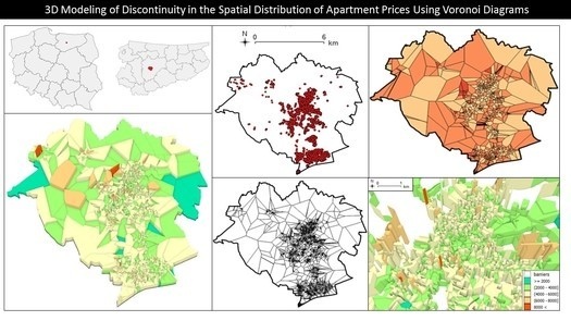
2.1. Description of Research Area

The study was conducted in the north-eastern part of Poland, in the city of Olsztyn (Warmińsko-Mazurskie Voivodeship)—Figure 1.
The city is currently inhabited by about 180,000 people in the area of almost 90 km2. The city has four rivers flowing through it; there are 15 lakes within its boundaries (9% of the city area), and a large part of its area is covered by forested areas and municipal greenery (including two nature reserves, Mszar and Redykajny)—58% of urban areas. These objects, along with industrial areas, generate a specific spatial structure, which, to a large extent, determines the spatial distributions of apartment prices (Figure 2).

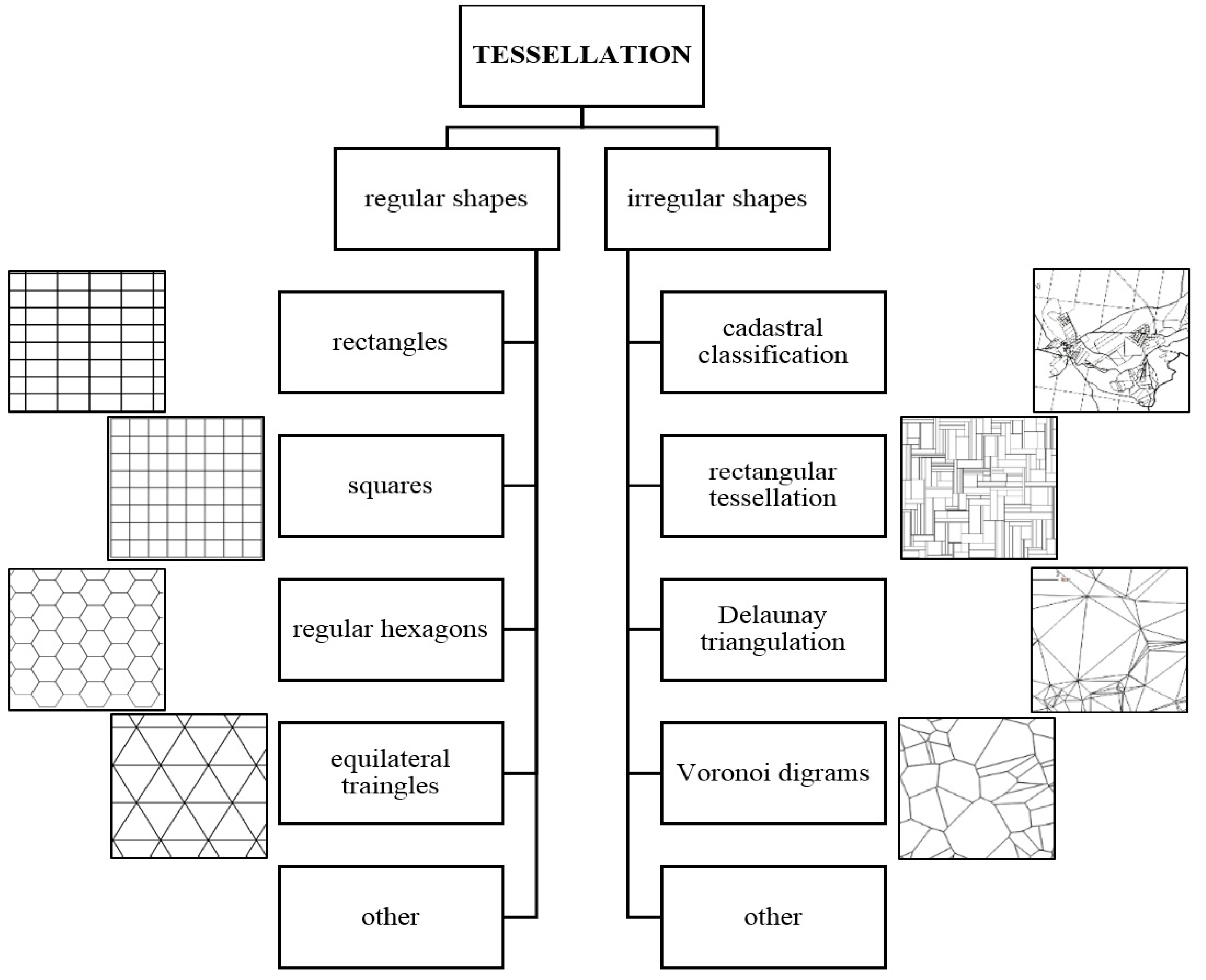
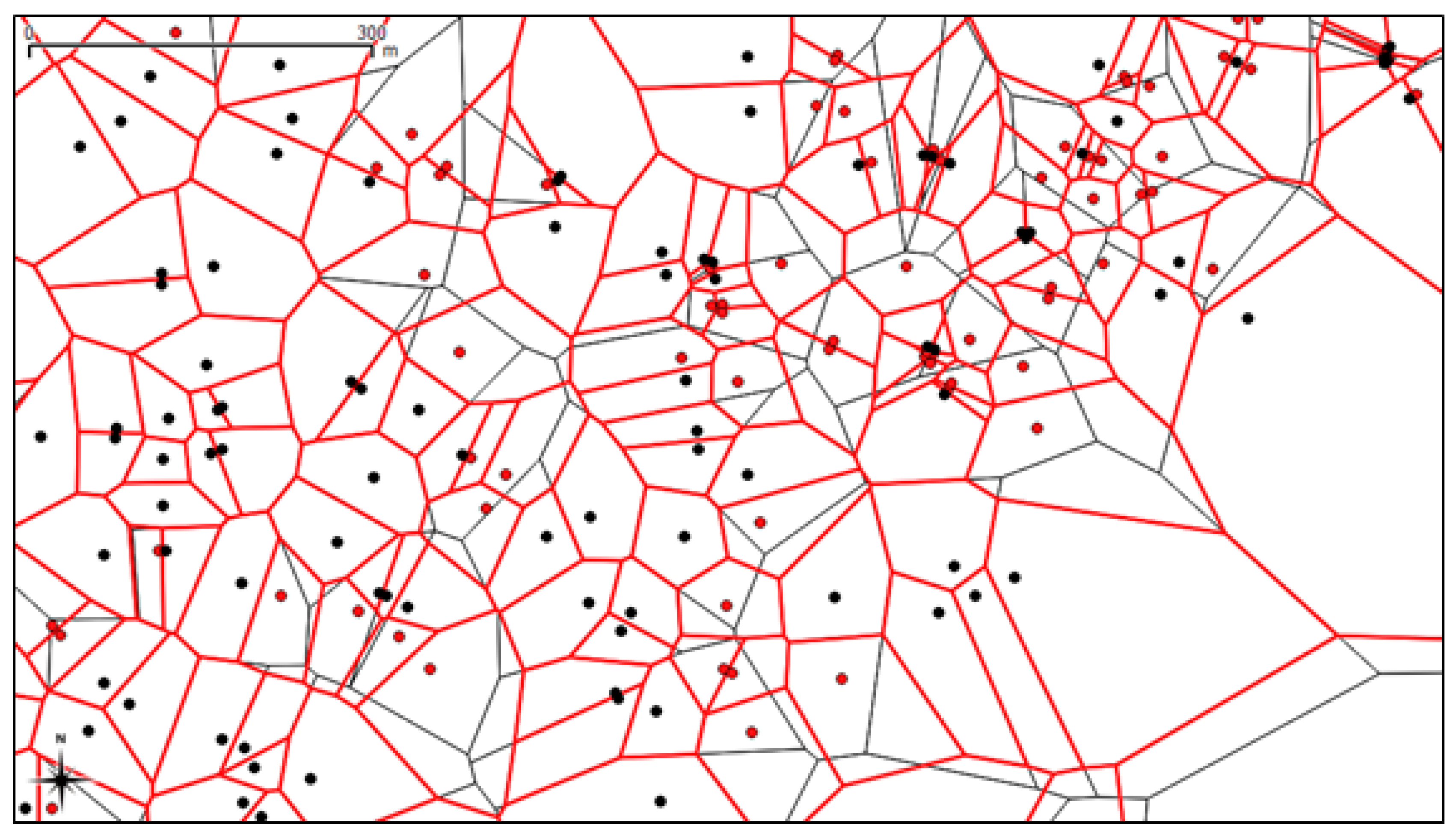
2.2. Research Methodology—Voronoi Diagrams

The conducted study proposed the application of irregular divisions of an Euclidean space through the use of the so-called Voronoi diagrams that are one of the numerous methods of spatial tessellation. Tessellation is understood as a method consisting of the division of a selected surface or space into a set of pre-defined geometric figures, which fill this area completely without leaving gaps or creating overlapping shapes [20,21]. The polygons formed in this way are referred to as cells, and the set of points on which they are based, to seeds, or nuclei [22]. The geometry of cells defined in this way (size, shape, orientation), as well as their spatial distribution (regularly or irregularly grouped patterns), maybe a tool for the identification of hierarchical relationships within spatial arrangements in relation to the attributes, both typically geographical and social phenomena. Spatial tessellations are extremely broadly used in a number of research areas, which translates into a significant increase in the publication activity while using tools of this type for, inter alia, the following:
(1)
model the Earth’s crust and the surface of water bodies [23];
(2)
make corrections of the area whose topography is represented by triangular solids [24];
(3)
visualize the catastrophe and natural disaster sites in order to establish a rescue system [25];
(4)
analyze environmental pollution [26];
(5)
examine the population’s education and income levels in a selected area [19];
(6)
model the areas of urban [27] and rural settlement [28];
(7)
map the morphology of human settlements, and to monitor the expansion of urbanized areas [29];
(8)
map the areas contaminated with barium or titanium found in paints [30];
(9)
generate optimal grids for object modeling [31];
(10)
examine real estate prices and their dynamics [19].
As a rule, tessellation is divided into methods based on regular or irregular shapes [22,32], as shown in Figure 3.
Regular tessellations are divisions of highly symmetrical spaces, which comprise congruent polygons with regular shapes that include equilateral triangles, squares, and regular hexagons [19]. Classical theories of spatial economy, i.e., theories by Christaler, Lösch, Berry, and Isard, are based on regular geometric figures, with particular emphasis on hexagons. The so-called hexagonal lattices satisfy two principles of spatial optimality, i.e., the principle of boundary length minimization and the principle of transport minimization; this type of tessellation has been widely used among city planners, spatial planners, and architects.
However, methods based on regular shapes have many limitations, particularly in the context of mapping the space presented using irregularly distributed phenomena. A major problem is the inflexibility of such structures at various levels of the aggregation of data concerning actual phenomena. Such observations are inherently too complex for regular grids, which usually result in lower accuracy of the models being generated, primarily those addressing the dynamics and relationships between the presented phenomena [19]. According to Kraus [34], the discretization of space through its regular division using simple geometric figures had numerous limitations, and the use of irregular polygons enabled the fitting of tessellation to the studied phenomenon or area in a more flexible manner. Assuming the regular division of the space in the study referred to the natural human tendency to simplify heterogeneous space towards the maximization of regularity and simplicity of the applied reality models. However, according to the authors of this study, regular forms of space fragmentation did not reflect the dominant irregularities in the real world. With reference to the housing market, which was the object of research in this study, the irregular tessellation preferred by the authors might be an appropriate tool for analyzing the activity of this market. This article adopted the assumption that Voronoi diagrams enabled, through the application of irregular division of areas on local housing markets, the visualization of the spatial aspect of the phenomena occurring on the housing market in a manner similar to their actual heterogeneous character, particularly in the case of dispersed data or a small volume of them.
Voronoi diagrams are a method for dividing Euclidean space [35], which takes into account the relationships between points and their surroundings when they are combined into groups as a result of context generalization based on the similarity of geographical structures of the analyzed area [36]. This division is the so-called natural tessellation, i.e., dividing a larger plane with points scattered onto it into non-overlapping areas in the form of polygons [21], by assigning each of its fragments to the nearest one of the set of the so-called generating points [37], in accordance with the spatial structure of the set under study [38]. Each point is assigned to one region in the form of a convex polygon (so-called Voronoi cell), to which it is situated closer than to any other polygons of the diagram [39]. This means that inside a particular Voronoi cell, the distance to the generating point of a particular cell is shorter than that to generating points of any other cells [40].
Voronoi diagrams can be defined as a set of vertices N = { n 1 ,   n 2 , ,   n M } with pre-defined Cartesian coordinates in d , where d is a d -dimensional Euclidean space [41]. Voronoi diagram of a set N is a division of the space into regions T I (Voronoi cells) in accordance with the Equation (1):
T I = { x d : d ( x ,   x I ) < d ( x ,   x J ) J I }
where: d ( x , x I ) = ( x 1 x I 1 ) 2 + ( x 2 x I 2 ) 2 —Euclidean distance, being the distance between x (the analyzed point) and x I (an i -th neighboring point chosen for the comparison). The set of n points, formed in this way, has a maximum of 2 n 5 vertex and 3 n 6 edges, and each of the vertices is, at the same time, the center of a circle circumscribed on at least three points located within the neighboring cells [42]. The process of formation of a Voronoi diagram can be described as follows [43]: where points p and q are available, they are connected with a section whose mid-perpendicular divides the space into two halves, each of which contains an area closer to each of the generating points. This operation is repeated for all possible pairs of points that are the closest neighbors of one another. The intersections between the obtained mid-perpendiculars form cells assigned to each of the points of the set, and the resulting grid of polygons is called a Voronoi diagram.
According to Guruprasad and Ghose [44], the main reason for the development of the method for dividing the space using Voronoi diagrams was to explain and describe various heterogeneities by determining local concentrations or clusters in order to obtain quantitative measures of system homogeneity [33] through forming groups with identical values of a selected feature [36]. They allowed one to observe the links between the vertices of particular areas, offer a certain overview of the topography of the studied area, and provide information on the neighborhood of selected points and its characteristics [45]. This is because the non-homogeneity of space requires, for cognitive reasons, that it is divided into elements with an identical structure, clearly distinguishable from the other parts of the area under study [11]. The most significant characteristic of this method is the possibility of preserving the original data despite their processing, and, primarily, for surviving the unavoidable smoothing in connection with the spatial distribution of data and avoiding additional smoothing due to interpolation of the analyzed values [24].

2.3. Data Collections
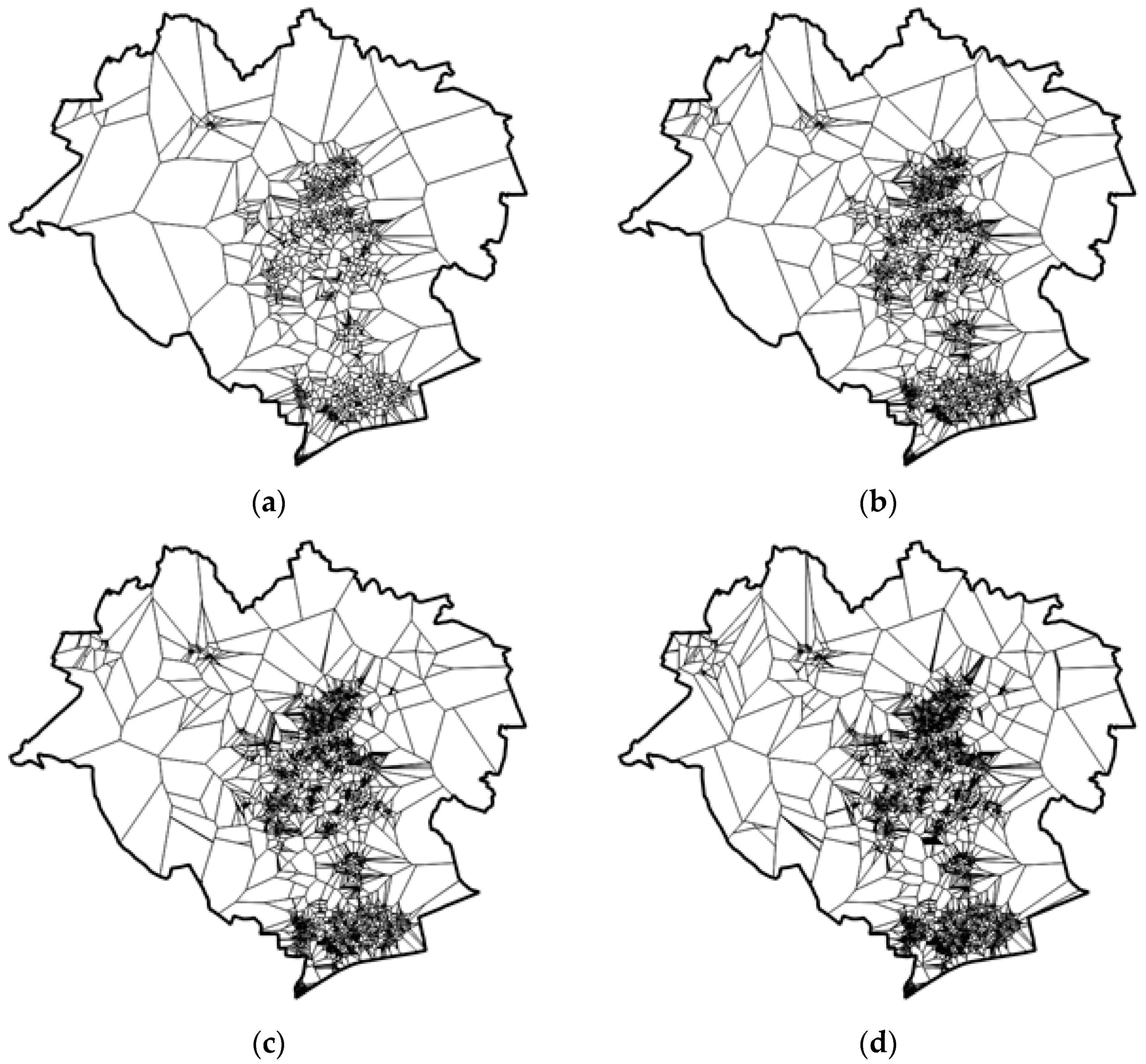
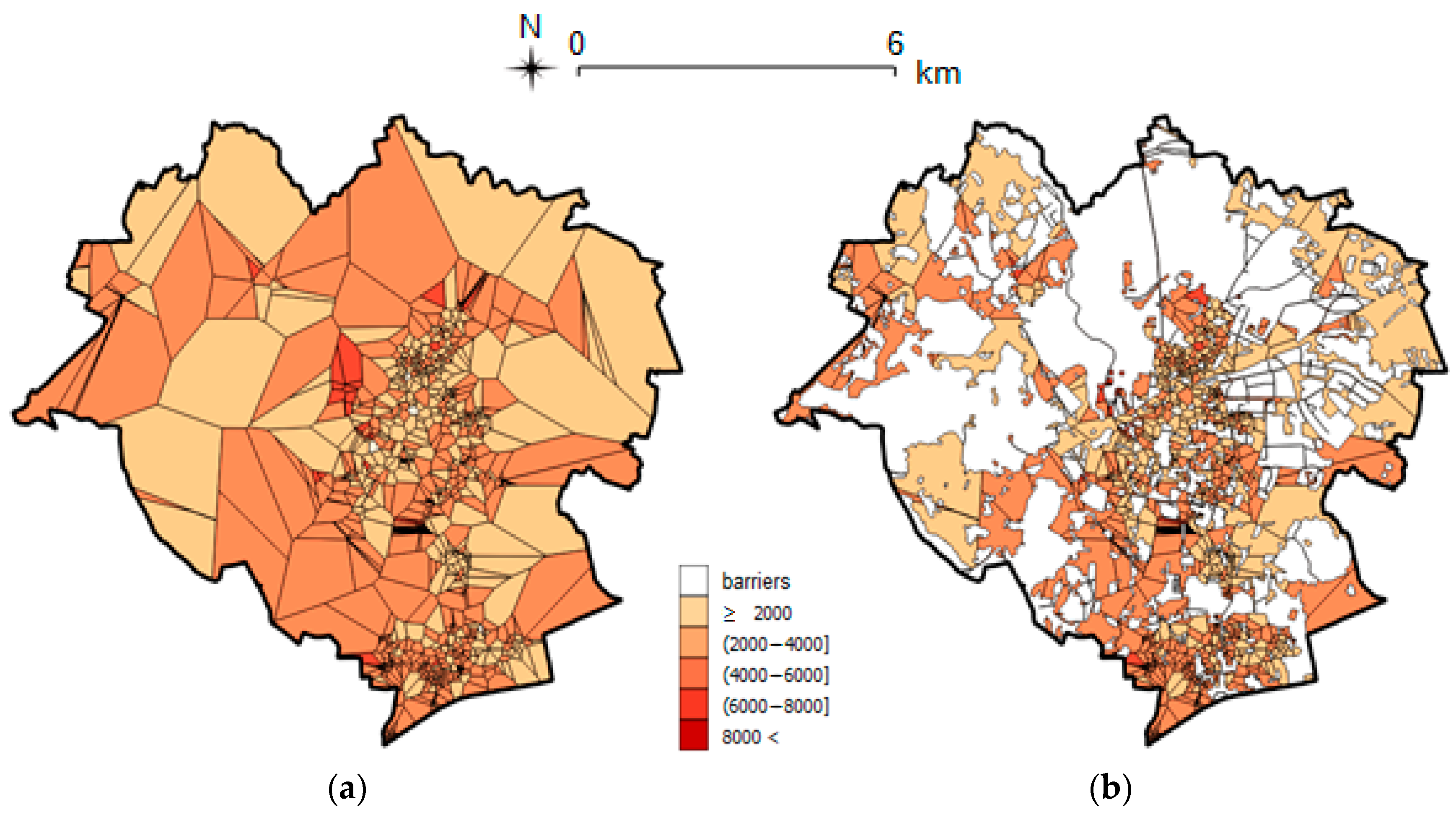
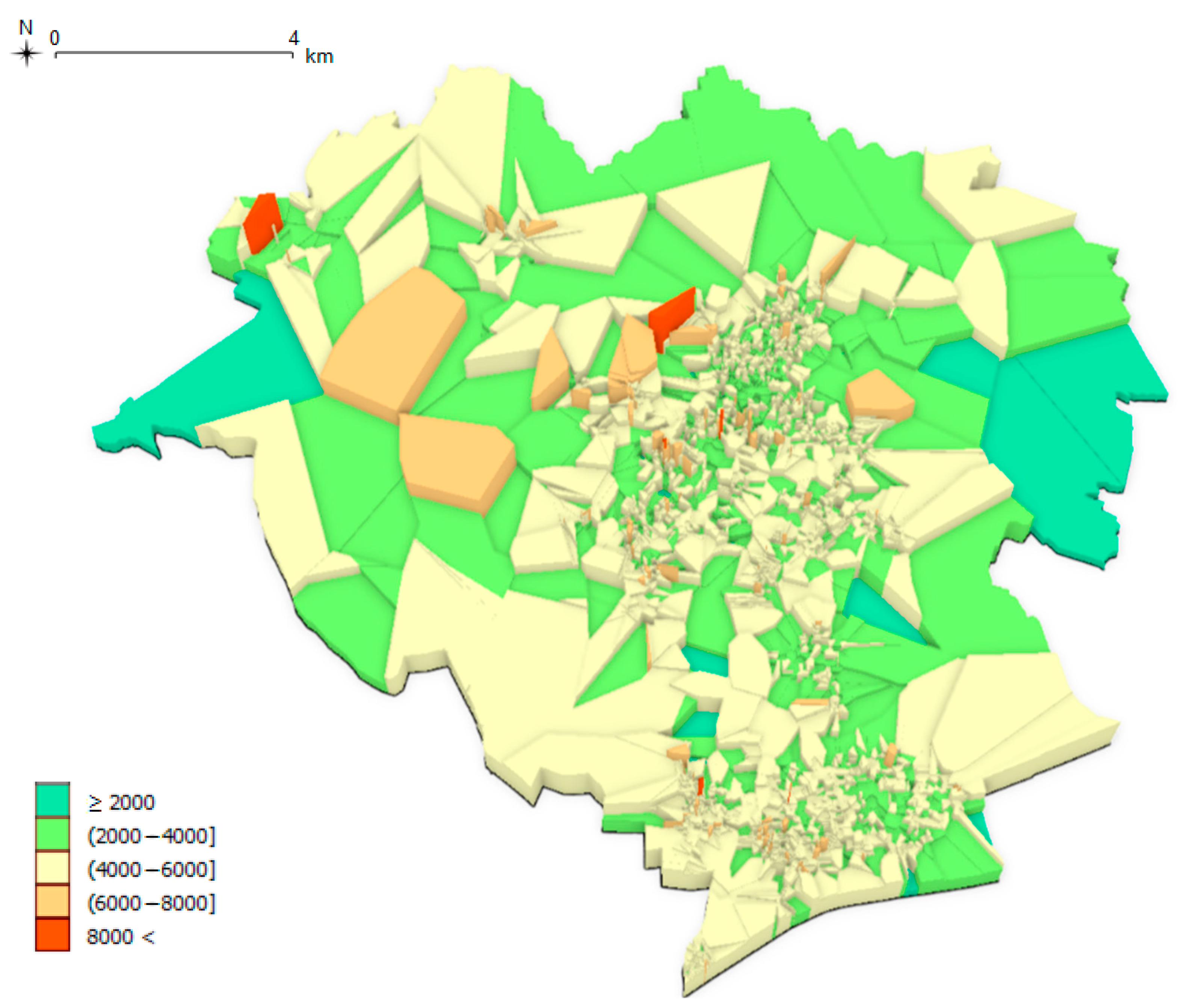
The source of data on apartment sale and purchase transactions was the real estate price and value register (RCiWN) maintained by the Olsztyn municipal office. These transactions concerned the ownership rights to residential properties sold on the free market and originating from the secondary market, where natural persons were parties to the transaction. The time horizon covered a period from 1 January 2010 to 31 December 2017. Figure 4 presents the procedure for the preparation of data necessary to generate a three-dimensional model of discontinuity in the spatial distribution of apartment prices using Voronoi diagrams.
In the first stage of the procedure (Figure 4), data on apartment prices were collected from the city of Olsztyn real estate price and value register in the form of an XLSX file. After completing the process of removing incomplete records and unifying the entries, 7303 transactions were obtained in the database formed in this way. This was followed by the determination of basic statistics (Table 1).
The calculated statistical measures showed that the arithmetic mean of prices for an apartment during the analyzed period (2010–2017) amounted to approx. 4200 PLN/m2 (ca. 980 EUR/m2), with the most frequently noted price (dominant) of 5000 PLN/m2 (ca. 1200 EUR/m2). The variation coefficient of 21% indicated low but statistically significant non-homogeneity of the collected data. Furthermore, in this case, we were dealing with left-sided asymmetry (negative values of the asymmetry index and skewness index, exceeding the value of 1), which means that the symmetrical distribution of the studied parameters around the mean value does not occur too often in reality. The kurtosis value indicated a flattened number curve and a small concentration of values around the mean value. After importing data to a QGIS software (Open Source Geographic Information System), the next stage of work was the so-called geocoding of addresses of each of the 7303 apartment sale prices in order to determine the geographical coordinates of the analyzed transactions.
OpenStreetMap and Google Maps services used for the geocoding failed to find some addresses; it was necessary to manually indicate the location of these transactions, followed by the verification of result correctness for the remaining part of the set. The final stage of the preparation of data for the construction of a three-dimensional model of discontinuity in the spatial distribution of apartment prices using Voronoi diagrams was the compilation of both a map of spatial distribution of apartment prices in Olsztyn and a map of the number of transactions in particular districts (administrative units in the city), presented in Figure 5.
The spatial distribution of 7303 prices of apartments in Olsztyn in the years 2001–2017, presented in Figure 5, confirmed the previously presented considerations, concerning the specificity of housing markets. What was clearly visible was the irregular dispersion of apartment sale transactions, as well as the occurrence of near-distance accumulations of smaller or larger price clusters. One of the reasons for this state of affairs is the rather complex spatial structure of the city of Olsztyn, which includes a lot of natural (forested areas and waters) and anthropogenic obstacles (industrial areas). The location of demand activity on the housing market could, therefore, be observed only outside these areas. For this reason, one needs to be aware that traditional methods of data interpolation that are aimed at the generation of continuous surfaces, in the case of such empirical data as those shown in Figure 5a, could generate significant uncertainty of the correctness of value maps compiled in this way. Based on the results of an analysis of the number of transactions in particular districts of Olsztyn (Figure 5b), it could be noted that most transactions were concluded during the period under study in the southern part of the city (from 752 to 328 transactions in a single unit), in the years 2001–2017. This area is a relatively new part of the city (housing estates: Jaroty, Generałów, Brzeziny, and Nagórki), which includes a significant number of residential buildings.

3. Results

The aim of the study was to search for the spatial discontinuity of apartment price distribution through the application of Voronoi diagrams as a method of irregular division of the space and to 3D visualize this discontinuity. In order to accomplish the task formulated in this way, after the preparation of spatial data from the years 2001–2017 for the city of Olsztyn (see: Section 2.3), a number of analyses were conducted using QGIS and ArcGIS Pro Software (accumulation of transactions). The first step was to conduct tessellation, i.e., the Olsztyn city area was divided into a grid of irregular polygons, the so-called Voronoi cells, in which each of the generating points (an apartment price) formed its polygon. The addition of more so-called generating points to the existing Voronoi diagram grid resulted in the generation of new links and, consequently, a new structure. The process of adding subsequent points and generating new Voronoi diagrams for particular years, defined in this way, is presented in Figure 6, based on the example of changes in the data structure in the years 2010–2011.
The applied procedure for cumulating data (apartment prices) from subsequent years enabled the visualization of the housing market activity in Olsztyn in the years 2010–2017. Figure 7 presents changes in the polygon mesh structure (Voronoi diagrams) in particular years.
Figure 7 shows the distribution and number of transactions in the city of Olsztyn using mesh size and density. The largest clusters of Voronoi cells were formed in the central and southern parts of the city, which coincided with both the distribution of residential buildings in its area and the number of transactions recorded in particular districts (Figure 5b).
Another stage of work was to generate the fields of apartment value in Olsztyn by combining Voronoi diagrams with chorochromatic maps. The combination of these methods enabled the presentation of the studied feature’s spatial diversity in the analyzed area through color differentiation in accordance with the value selected for visualization. Consequently, non-classical maps of apartment values were obtained through the application of irregular tessellation with Voronoi diagrams (Figure 8a). To improve the readability of the generated maps, it was decided to aggregate cells in accordance with the adopted five-point scale. At the same time, in reference to the Five Principles of Spatial Econometrics [46], which address the need to take into account topographical elements in the two-dimensional spaces being created (see Section 4), a value map was compiled using irregular tessellation with Voronoi diagrams, including forested areas, waters, and industrial areas (Figure 8b).
In the classical interpolation methods (see Section 4), the observation of the value map prevented the assessment of the reliability of the obtained value level. As regards the proposed method, i.e., an irregular tessellation with Voronoi diagrams and chorochromatic maps (Figure 8a), an observer of the map constructed in this way could unambiguously assess the risk levels for the generated apartment values. The rule should be adopted that the larger the Voronoi cells are, the higher the number of transactions in these areas and, consequently, the lower the reliability of the obtained real estate values. The inclusion of topographical elements, i.e., green areas, waters, and industrial areas in which no apartment sale transactions could be conducted, brought one closer to modeling actual spatial relationships in urbanized areas. The map of apartment values in Olsztyn, presented in Figure 8b, through such a “rough” visualization was rather difficult to accept for recipients accustomed to value maps based on the spatial continuity applied, as a rule, in classical interpolation models. However, the form of visualization defined in this way did not suggest to the recipient unrealistic phenomena, i.e., unambiguously defined apartment value levels in the area of forests or lakes.
The next stage of geospatial analysis of apartment values in Olsztyn in the years 2010–2017 was the procedure for spatial visualization in the form of a 3D model using the so-called solid cartogram (blockogram). An analysis of discontinuity zones (areas with big abrupt changes in the value on field boundaries) enabled the localization of areas, which require particular attention (uncertainty zones), mainly in terms of determining intermediate values between particular generating points. Figure 9 presents a 3D model of apartment prices in Olsztyn in the form of a solid cartogram using irregular tessellation with Voronoi diagrams.
On the other hand, Figure 10 and Figure 11 present a smaller part of the urban space of the city of Olsztyn, in which differences are demonstrated between 3D models, both including and excluding wooded areas, waters, and industrial areas. Such a comparison on a small fragment of the city part allowed one to realize, to a greater extent, the so-called spatial discontinuity of apartment prices and, at the same time, informs of the significant impact of topographical elements on the shaping of the spatial distribution of these prices.
The three-dimensional maps of apartment values in Olsztyn, presented in Figure 9, Figure 10 and Figure 11, were distinctly different from the value maps compiled using classical interpolation models. The spatial discontinuity of apartment prices was clearly diagnosed, and the above-average apartment prices were not removed from the model in the smoothing process but were an integral part of this model. On the housing market, not each variable (as long as it is market-based) was a statistical error or a deviation from the norm (an average price), and this should be taken into account in spatial analyses of this market.
Figure 9, Figure 10 and Figure 11 show the prices of apartments (red) of more than 8000 PLN/m2 (ca. 1850 EUR/m2) at a distance of less than 0.1 km from the cluster of prices (green), ranging from 2000 PLN/m2 to 4000 PLN/m2 (from ca. 460 EUR/m2 to ca. 930 EUR/m2). Such significant price disparities are an inherent feature of the housing market and should not be reduced by various forms of smoothing in order to create a continuous surface of the value map. The occurrence of discontinuity zones and hyper-outlying prices on the three-dimensional model in the city of Olsztyn was much more evident than in the case of 2D imaging. The inclusion of numerous field obstacles (forested area, waters, and industrial areas) showed that omitting this issue in research into the housing markets could lead to serious abuse, particularly during analyses of land with such an irregular distribution of the set of points concerned. As regards newer residential buildings that are often characterized by considerably higher prices than neighboring older buildings, such an approach enabled the search for similar objects at appropriate levels, which were distinct zones in the 3D model. According to Zhang [47], three-dimensional analysis methods had obvious advantages over two-dimensional approaches, especially for multi-information presentation and complex spatial analysis. Previous research on urban housing prices mainly used kriging and co-kriging techniques for price prediction, while the application of geo-visual analytics is rare, especially for the analysis and visualization of non-linear complex urban spatial structures and spatial morphology.

4. Discussion

The formation of value fields on the basis of irregular tessellations in the form of Voronoi diagrams, proposed in this article, and the subsequent 3D visualization procedure, are an innovative method for identifying clusters of the demand zone of high activity on the housing market and for identifying the areas of above-average prices, which are, as a rule, removed from interpolation models as hyper-outlying ones. The research concept presented in this way refers to the main ideas of the systemic approach (4C: complexity, chaos, catastrophe, cybernetics) [48,49,50,51,52]. The presented paper promoted greater methodological pluralism (in the spirit of holism, realism, and limited rationality), which is characterized by greater openness in searching for alternative solutions while applying interdisciplinary research methods. Such an approach facilitates research into untypical economic phenomena within the urbanized space of cities. The theoretical basis of the conducted research, in the broadest theoretical context, has been discussed in the further part of this chapter.
In the simplest terms, the geospatial analysis focuses on the presentation of spatial relationships, description of data distribution, and searching for standards, clusters, and outlying observations in a pre-defined area [53,54]. It deals with various computational transformations and procedures, which result in an appropriate preparation of spatial information, which allows scientific problems to be solved [55] or complex decision-making models to be constructed [56]. The basic assumptions used in geospatial analyses are so-called Tobler’s First Law of Geography and Five Principles of Spatial Econometrics.
According to the First Law of Geography [57], everything is related to everything else, but those which are near to each other are more related when compared to those that are further away. On the other hand, according to the Five Principles of Spatial Econometrics [46], spatial research should take the following into account:
(1)
spatial interdependence;
(2)
spatial asymmetry in the measures of spatial interdependence;
(3)
Allotopy—the influence of exogenous variables from another spatial localization;
(4)
ex-post interaction being different from ex-ante interaction;
(5)
two-dimensional space, containing topological elements.
The above-mentioned fundamental laws of spatial analyses, which are the essence of a number of empirical scientific studies [58,59,60,61], essentially address the problem of generating continuous spatial structures from the set of dispersed points. In its essence, space has a continuous [23,38] and not discrete (discontinuous) form; however, in reality, it is practically impossible to obtain an appropriate number of observations in order to obtain such continuity [19,62]. Consequently, a number of procedures are obtained from the non-homogeneous set of empirical data, which in reality aim at assigning appearances of continuity to the studied phenomena emanations that are of discontinuous (discrete) nature. Many spatial data are observed in irregularly distributed locations [63,64], with the simultaneous occurrence of significant clusters of these data, as well as zones completely devoid of them. As a result, in the processes of generating a continuous spatial distribution of the studied phenomenon, various levels of data quality are involved. In certain zones, the spatial analysis is based on a few spatial data, while, in other zones, it generates continuity based on a few dozen or a few hundred. Obtaining spatial continuity from the dispersed and non-homogeneous spatial data is based on various interpolation methods [62,65].
The interpolation of spatial data [55] is defined as a “process of intelligent speculating”, which, according to Okabe [27], involves the determination of reasonable estimates of the value of space in locations in which no observations have been carried out, based on known values occurring within their surroundings. Interpolation consists of finding an appropriate function (so-called interpolant), which transforms numerical values of single operations into a continuous or more densely sampled surface [55] in order to visualize the way in which the phenomena observed in the form of point data may be distributed over a pre-defined area within the space [66]. Interpolation procedures can be divided into:
(1)
deterministic—which are models comprised of functions based on the distance or surface, which determine the particular mathematical surface, inter alia inverse distance weighted method, polynomial interpolation, nearest neighbor method, natural neighbor method, quasi-natural interpolation, radial basis functions, or spline functions;
(2)
stochastic (geostatistical)—which are based on stochastic models and take into account data autocorrelation, which allows them to assess errors in the obtained results and to assess the probability of the occurrence, in a particular place, of values differing from the pre-specified threshold value along with the compilation of maps, which illustrate this situation, inter alia the kriging or areal interpolation.
According to Zhang [41], with the rapid development of GIS technologies and the gradual evolution towards geographical information science [67], an increasing number of studies introduced the GIS-based spatial analysis methods for analyzing spatial characteristics of urban housing. Spatial interpolation methods (such as kriging or inverse distance weighted method) are often used to estimate the land price in an unknown area in a city [68,69]. It can be stated that classical interpolation methods are a proven and appropriate method for generating the continuity of the studied phenomenon from discontinuous spatial data; however, the spatial distribution visualizations obtained in this way imply the uniform level of confidence in results within the entire area under study. Regarding the housing market, as mentioned above, the distribution of prices is not uniform. In such a case, there are various levels of confidence in the obtained results of classical interpolations, which implies the need for a scientific discussion about this issue.
A significant feature of the structures occurring on the housing market is the high dispersion of points, and the spatial development of real estate prices is not regular or equidistant. At the same time, irregular accumulations of near-distance observations (apartment prices) are observed in the form of single, small groups. The obvious is the fact that the urban spatial structure is becoming more and more complicated. It is difficult to describe and interpret urban spatial characteristics with the monocentric hypothesis and simple linear models [70]. According to Zhang [47], recent research has focused on the polycentric urban region in urban studies [71,72,73] as polycentric urban development morphology is becoming a trend [74]. In this study, the authors attempted to focus more on the issues of discontinuity than on the creation of continuity (interpolation) from the set of discrete spatial variables. The originator of the catastrophe theory (also known as the theory of discontinuous passages or morphogenesis theory), Thom [75], claimed that each science is the examination of certain morphologies, with these morphologies being contained within a certain space, which is usually our space-time continuum or any space that originates from it, and the interesting issue should primarily be the significant components of these morphologies, i.e., discontinuities. Discontinuities, or transition zones, are ubiquitous [76] and are potentially important in maintaining biodiversity [77,78]. Discontinuity occurs where a set of system behaviors is divided into qualitatively different types, and transitions between them appear due to continuous changes in the set of causes [79].
Observation of empirical data from housing markets (dispersion, irregularity, various cluster levels) demonstrates the actual certain misfit to Tobler’s First Law of Geography (similarity of close objects) to the phenomena occurring on this market. According to this law [57], in the case of apartment price clusters, the concentration of similar apartment prices should be observed since the closer objects are more dependent on one another than the distant ones. However, prices of apartments in the immediate vicinity can be substantially different, which generates the creation of the so-called price peaks and depressions (a natural phenomenon on housing markets). As a rule, the classical methods of spatial data interpolation [80,81] usually fail to tackle the issue of hyper-outlying prices of apartments while determining the smoothing process and, consequently, eliminate such data from the database. A result of such a procedure is the correctly constructed interpolation of maps of apartment prices or values in a particular urbanized zone, which, however, does not represent the actual specificity of the housing market.
The source of the occurrence of hyper-outlying prices of apartments (in the same location) is the qualitative non-homogeneity of residential buildings, which corresponds to the substantially different positions of potential purchasers in the social hierarchy. This phenomenon intensified, following the international financial crisis of 2007–2008, when the access to financing sources was restricted, the uncertainty of employment and long-term maintenance of high incomes increased, and the investment opportunities for the wealthy section of society relatively decreased. Consequently, the search for investment areas in the vicinity of city centers intensified, which contributed to a change in the classical suburbanization process. A part of society with high incomes generated pressure on the quality of the construction matter of new developer’s investments, as the abandonment of settling outside the urban zone did not mean, at the same time, a reduction in requirements as regards the architectural quality, finish of the building, shared spaces of the building or its surroundings. At the same time, this pressure on the (developers’) supply sphere created a trend for searching for free areas designated for residential development in the city’s central zones. This resulted directly from the purchasers’ expectations, for whom an alternative was a house within the rural space zone, including the inconveniences of transport to a workplace located within the urban space zone. Consequently, next to similar civil structures constructed using similar technologies, with similar apartment prices on the secondary market, modern luxury apartment buildings were constructed, whose apartment prices significantly exceeded average local prices. The result of such processes is the observation of the principal price non-homogeneity of residential buildings located close to one another.

5. Conclusions

The study promoted greater methodological pluralism (in the spirit of holism, realism, and limited rationality), which is characterized by greater openness in searching for alternative solutions while applying interdisciplinary research methods. Consequently, the authors fully accepted the complexity and non-linearity of spatial relationships that are dominant in the real world and accepted spatial discontinuity as an inherent feature of the housing market.
In contrast to classically applied interpolation methods that create problems in geospatial analyses typical of the housing markets of highly diversified areas, this study assessed the possibility of implementing irregular tessellation methods for this purpose. Particular attention was paid to the Voronoi diagrams, which enabled the identification of local clusters of the studied phenomena within the heterogeneous space. The proposal of 3D visualization of the real estate price spatial distribution presented in the article, which takes into account the occurrence of discontinuity zones, might prove to be a significant innovation in research into the housing market and affect the effectiveness of economic decision-making. The methods applied in the study enabled avoiding excessive generalization, as well as obtaining false results or their over-interpretation due to an excessive reduction in above-average values. The effect of such an approach was the appropriate representation of real estate specificity, as well as the reflection of the heterogeneous character of reality, with account taken of the occurrence of areas permanently excluded from market activity or characterized by its high activity and the existence of hyper-outlying areas with prices significantly deviating from those observed in the neighborhood. The basic effect of the study, determining its innovative character, was the visualization of spatial discontinuity of the real estate price distribution using 3D modeling, which enabled the identification of high activity clusters and areas with high prices, which were, as a rule, removed from interpolation models as hyper-outlying ones.
The authors were aware that the proposed way of visualizing the spatial distribution of real estate prices was difficult for users accustomed to maps based on interpolation methods. This was one of the limitations of the proposed method. Another difficulty in the applicability of tessellation was that, contrary to interpolation methods, results of using Voronoi diagrams were not a form of a continuous function. They were a set of discrete cells with assigned attributes, joined with each other on the basis of their neighborhood. This could affect the quite rapid changes of values at the edges of particular cells, considered as areas of uncertainty, which increases the risk level of spatial analyses. On the other hand, however, classical interpolation methods also presented numerous limitations and disadvantages, which was the reason for our interest in Voronoi diagrams.
Thanks to the implementation of Voronoi diagrams, the results of geospatial analyses might provide real estate market participants with an initial overview of the market situation and supplement municipal or county spatial information systems (geoportals), tools used by real estate surveyors or real estate brokers (for preliminary identification of the market situation), or systems for examining applications for a mortgage loan (as a tool of initial data verification by banks). These results might also be a valuable source of information for local authorities by providing them with an overview of the current condition of the equipment in the area under their responsibility with public utility facilities and allowing them to plan changes in the space with the aim of adapting to society’s needs in this regard. They could also become part of the procedures related to making investment decisions concerning real estate management by interested parties, in accordance with the procedure proposed in the paper.

Author Contributions

Conceptualization, M.B., M.F.; Data curation, M.F.; Formal analysis, M.B., M.F.; Investigation, M.B., M.F.; Methodology, M.B., M.F.; Visualization, M.B., M.F. The participation of the first two authors is equal in value. All authors have read and agreed to the published version of the manuscript.

Funding

This research received no external funding.

Acknowledgments

The authors express sincere gratitude to the Journal Editor and the anonymous reviewers who spent their valued time to provide constructive comments and assistance to improve the quality of this paper.

Conflicts of Interest

The authors declare no conflicts of interest.

References

  1. Rutten, R.; Westlund, H.; Boekema, F. The spatial dimension of social capital. Eur. Plan. Stud. 2010, 18, 863–871. [Google Scholar] [CrossRef] [Green Version]
  2. Tozzi, A.; Peters, J.F. Towards a fourth spatial dimension of brain activity. Cogn. Neurodyn. 2016, 10, 189–199. [Google Scholar] [CrossRef] [PubMed]
  3. Hellerstein, J.K.; Kutzbach, M.J.; Neumark, D. Do labor market networks have an important spatial dimension? J. Urban Econ. 2014, 79, 39–58. [Google Scholar] [CrossRef] [Green Version]
  4. Kulesza, S.; Bramowicz, M. A comparative study of correlation methods for determination of fractal parameters in surface characterization. Appl. Surf. Sci. 2014, 293, 196–201. [Google Scholar] [CrossRef]
  5. Cellmer, R. Use of spatial autocorrelation to build regression models of transaction prices. Real Estate Manag. Valuat. 2013, 21, 65–74. [Google Scholar] [CrossRef] [Green Version]
  6. Senetra, A.; Szczepańska, A.; Wasilewicz-Pszczółkowska, M. Analysis of changes in the land use structure of developed and urban areas in Eastern Poland. Bull. Geogr. Socio Econ. Ser. 2014, 24, 219–230. [Google Scholar] [CrossRef] [Green Version]
  7. Arnott, R. Optimal city size in a spatial economy. J. Urban Econ. 1979, 6, 65–89. [Google Scholar] [CrossRef]
  8. Domański, R. Ewolucyjna Gospodarka Przestrzenna; Wydawnictwo Uniwersytetu Ekonomicznego w Poznaniu: Poznań, Poland, 2012. [Google Scholar]
  9. Fujita, M.; Krugman, P.R.; Venables, A. The Spatial Economy: Cities, Regions, and International Trade; MIT Press: Cambridge, MA, USA, 1999. [Google Scholar]
  10. Hagett, P. Alternative futures, problems and possibilities. In Directions in Geography; Chorley, R.J., Ed.; Methuen Publisher: London, UK, 1973; pp. 219–235. [Google Scholar]
  11. Kuciński, K. Geografia Ekonomiczna. Zarys Teoretyczny; Wydawnictwo Szkoła Główna Handlowa: Warszawa, Poland, 1994. [Google Scholar]
  12. Williamson, I.P. Land administration “best practice” providing the infrastructure for land policy implementation. Land Use Policy 2001, 18, 297–307. [Google Scholar] [CrossRef] [Green Version]
  13. Gross, M.; Źróbek, R. Good governance in some public real estate management systems. Land Use Policy 2015, 49, 352–364. [Google Scholar] [CrossRef]
  14. Enemark, S.; van der Molen, P. A framework for self-assessment of capacity needs in land administration. In Proceedings of the International FIG Congress; International Federation of Surveyors: Munich, Germany, 2006. [Google Scholar]
  15. Dawidowicz, A.; Źróbek, R. Land Administration System for Sustainable Development–Case Study of Poland. Real Estate Manag. Valuat. 2017, 25, 112–122. [Google Scholar] [CrossRef] [Green Version]
  16. Ball, M. Housing Policy and Economic Power: The Political Economy of Owner Occupation; Routledge: Abingdon, UK, 2017. [Google Scholar]
  17. Beltratti, A.; Morana, C. International house prices and macroeconomic fluctuations. J. Bank. Financ. 2010, 34, 533–545. [Google Scholar] [CrossRef]
  18. Orenstein, D.E.; Hamburg, S.P. Population and pavement: Population growth and land development in Israel. Popul. Environ. 2010, 31, 223–254. [Google Scholar] [CrossRef]
  19. Mostafavi, M.A.; Beni, L.H.; Mallet, K.H. Geosimulation of Geographic Dynamics Based on Voronoi Diagram. In Transactions on Computational Science IX. Special Issue on Voronoi Diagrams in Science and Engineering; Gavrilova, M.L., Tan, C.J.K., Anton, F., Eds.; Lecture Notes in Computer Science; Springer: Berlin, Germany, 2010; Volume 6290, pp. 183–202. [Google Scholar]
  20. Bertram, M.; Duchaineau, M.A.; Hamann, B.; Joy, K.I. Wavelets on planar tessellations. In Proceedings of the International Conference on Imaging Science, Systems, and Technology (CISST 2000), Las Vegas, NV, USA, 26–29 June 2000; Volumes I and II, pp. 619–625. [Google Scholar]
  21. Ren, J.; Dijksman, J.; Behringer, R.P. Homogeneity and packing structure of a 2D sheared granular system. AIP Conf. Proc. 2013, 1542, 527–530. [Google Scholar] [CrossRef] [Green Version]
  22. Le Bera, F.; Lavigneb, C.; Adamczyk, K.; Angevin, F.; Colbache, N.; Mari, J.F.; Monod, H. Neutral modelling of agricultural landscapes by tessellation methods—Application for gene flow simulation. Ecol. Model. 2016, 220, 3536–3545. [Google Scholar] [CrossRef] [Green Version]
  23. Gold, C.M. Tessellations in GIS: Part I—Putting it all together. Geo-Spat. Inf. Sci. 2016, 19, 9–25. [Google Scholar] [CrossRef] [Green Version]
  24. Dos Santos, N.P.; Escobar, I.P. Discrete evaluation of Stokes’s integral by means of Voronoi and Delaunay structures. J. Geod. 2004, 78, 354–367. [Google Scholar] [CrossRef]
  25. She, B.; Zhu, X.; Ye, X.; Guo, W.; Su, K.; Lee, J. Weighted network Voronoi Diagrams for local spatial analysis. Comput. Environ. Urban 2015, 52, 70–80. [Google Scholar] [CrossRef]
  26. Liu, J.; Li, W.; Wu, J. A framework for delineating the regional boundaries of PM2.5 pollution: A case study of China. Environ. Pollut. 2018, 235, 642–651. [Google Scholar] [CrossRef]
  27. Okabe, A.; Boots, B.; Sugihara, K.; Chiu, S.N. Spatial Tessellations: Concepts and Applications of Voronoi Diagrams, 2nd ed.; Wiley Series in Probability and Statistics; John Wiley & Sons: Chichester, UK, 2000. [Google Scholar]
  28. Kisiała, W.; Rudkiewicz, M. Zastosowanie diagramu Woronoja w badaniu przestrzennych wzorców rozmieszczenia i dostępności sklepów dyskontowych. Przegląd Geogr. 2017, 89, 187–212. [Google Scholar] [CrossRef] [Green Version]
  29. Alhaddadn, B.I.; Burnsn, M.C.; Roca, J. Methods for monitoring the detection of multi temporal land use change through the classification of urban areas. In Proceedings of the International Archives of the Photogrammetry, Remote Sensing and Spatial Information Sciences, 28th Urban Data Management Symposium (UDMS 2011), Delft, The Netherlands, 28–30 September 2011; Volume XXXVIII 4/C21, pp. 83–86. [Google Scholar]
  30. Roff, M.; Bagon, D.A.; Chambers, H.; Dilworth, E.M.; Warren, N. Dermal Exposure to Dry Powder Spray Paints Using PXRF and the Method of Dirichlet Tesselations. Ann. Occup. Hyg. 2004, 48, 257–265. [Google Scholar] [CrossRef]
  31. Yan, D.M.; Wang, W.; Lévy, B.; Liu, Y. Efficient computation of clipped Voronoi diagram for mesh generation. Comput. Aided Des. 2013, 45, 843–852. [Google Scholar] [CrossRef] [Green Version]
  32. Cartwright, A.; Moss, J.; Cartwright, J. New statistical methods for investigating submarine pockmarks. Comput. Geosci. 2011, 37, 1595–1601. [Google Scholar] [CrossRef]
  33. Figurska, M.; Bełej, M. Teselacja jako metoda badania aktywności rynku mieszkaniowego. Biul. Stowarzyszenia Rzeczozn. Majątkowych Województwa Wielkop. 2018, 50, 18–28. [Google Scholar]
  34. Kraus, M.; Rajagopal, A.; Steinmann, P. Investigations on the polygonal finite element method: Constrained adaptive Delaunay tessellation and conformal interpolants. Comput. Struct. 2013, 120, 33–46. [Google Scholar] [CrossRef]
  35. Ai, T.; Yu, W.; He, Y. Generation of constrained network Voronoi diagram using linear tessellation and expansion method. Comput. Environ. Urban 2015, 51, 83–96. [Google Scholar] [CrossRef]
  36. Hangouët, J.F.; Djadri, R. Voronoi diagrams online segments: Measurements for contextual generalization purposes, Spatial information theory: A theoretical basic for GIS. Lect. Notes Comput. Sci. 1997, 1329, 207–222. [Google Scholar]
  37. Batista, M.R.; Calvo, R.; Romero, R.A.F. A Robot online Area Coverage Approach based on the Probabilistic Lloyd Method. In Proceedings of the IEEE International Joint Conference on Neural Networks, Dallas, TX, USA, 4–9 August 2013; pp. 2145–2152. [Google Scholar]
  38. Peterka, T.; Kwan, J.; Pope, A.; Finkel, H.; Heitmann, K.; Habib, S.; Wang, J.; Zagaris, G. Meshing the Universe: Integrating Analysis in Cosmological Simulations. In Proceedings of the SC Companion: High Performance Computing, Networking, Storage and Analysis, Salt Lake City, UT, USA, 10–16 November 2012; pp. 186–195. [Google Scholar] [CrossRef]
  39. Andronov, L.; Orlov, I.; Lutz, Y.; Vonesch, J.L.; Klaholz, B.P. ClusterViSu, a method for clustering of protein complexes by Voronoi tessellation in superresolution microscopy. Sci. Rep. 2016, 6, 1–9. [Google Scholar] [CrossRef] [Green Version]
  40. Różniatowski, K.; Kosmulski, M. Advanced Analysis of SEM Images of Carbon Ceramic Composites. Adsorpt. Sci. Technol. 2007, 25, 473–478. [Google Scholar] [CrossRef] [Green Version]
  41. Zhang, Y.; Yi, H.L.; Tan, H.P. Natural element method for radiative heat transfer in two dimensional semitransparent medium. Int. J. Heat Mass Transf. 2013, 56, 411–423. [Google Scholar] [CrossRef]
  42. Surendran, S.; Chitraprasad, D.; Kaimal, M.R. Voronoi Diagram-Based Geometric Approach for Social Network Analysis. In Computational Intelligence, Cyber Security and Computational Models; Krishnan, G.S.S., Anitha, R., Lekshmi, R.S., Kumar, M.S., Bonato, A., Graña, M., Eds.; Proceedings of ICC, Advances in Intelligent Systems and Computing; Springer: New Delhi, India, 2013; Volume 246, pp. 359–372. [Google Scholar]
  43. Watunyuta, W.; Chu, C.H. Voronoi tessellation-based spatial domain analysis of digital halftoning methods. Opt. Commun. 1997, 140, 110–118. [Google Scholar] [CrossRef]
  44. Guruprasad, K.R.; Ghose, D. Heterogeneous locational optimisation using a generalised Voronoi partition. Int. J. Control 2013, 86, 977–993. [Google Scholar] [CrossRef]
  45. Dattaa, A.; Duttab, S.; Pala, S.K.; Sen, R. Progressive cutting tool wear detection from machined surface images using Voronoi tessellation method. J. Mater. Process. Technol. 2013, 213, 2339–2349. [Google Scholar] [CrossRef]
  46. Klaassen, J.H.P.; Paelinck, L.H. Ekonometria Przestrzenna; PWN: Warszawa, Poland, 1983. [Google Scholar]
  47. Zhang, Z.; Lu, X.; Zhou, M.; Song, Y.; Luo, X.; Kuang, B. Complex spatial morphology of urban housing price based on digital elevation model: A case study of Wuhan city, China. Sustainability 2019, 11, 348. [Google Scholar] [CrossRef] [Green Version]
  48. Peters, E.E. Complexity, Risk, and Financial Markets; John Wiley & Sons: Hoboken, NJ, USA, 2001; Volume 84. [Google Scholar]
  49. Unold, J. Dynamika Systemu Informacyjnego a Racjonalność Adaptacyjna. Teoretyczno-Metodologiczne Podstawy Nowego Ujęcia Racjonalności; Wydawnictwo AE Wrocław: Wrocław, Poland, 2003. [Google Scholar]
  50. Holt, R.P.; Rosser, J.B., Jr.; Colander, D. The complexity era in economics. Rev. Polit. Econ. 2011, 23, 357–369. [Google Scholar] [CrossRef] [Green Version]
  51. Bełej, M. Catastrophe theory in explaining price dynamics on the real estate market. Real Estate Manag. Valuat. 2013, 21, 51–61. [Google Scholar] [CrossRef] [Green Version]
  52. Jakimowicz, A. Nowa Ekonomia: Systemy Złożone i Homo Compositus; Wydawnictwo Naukowe PWN: Warszawa, Poland, 2016. [Google Scholar]
  53. Haining, R. Spatial Data Analysis. Theory and Practice; Cambridge University Press: Cambridge, UK, 2004. [Google Scholar]
  54. Loonis, V.; Bellefon, M.P. Handbook of Spatial Analysis. Theory and Application with R; Montrouge Cedex: Montrouge, France, 2018. [Google Scholar]
  55. Longley, P.A.; Goodchild, M.F.; Maguire, D.J.; Rhind, D.W. Geographical Information Systems and Science, 2nd ed.; John Wiley & Sons, Ltd: Chichester, UK, 2005. [Google Scholar]
  56. Gotlib, D.; Iwaniak, A.; Olszewski, R. GIS. Obszary Zastosowań; Wydawnictwo Naukowe PWN: Warszawa, Poland, 2007. [Google Scholar]
  57. Tobler, R.W. A computer movie simulating urban growth in the Detroit region. Econ. Geogr. 1970, 46, 234–240. [Google Scholar] [CrossRef]
  58. Edgington, W.D.; Hyman, W. Using baseball in social studies instruction: Addressing the five fundamental themes of geography. Soc. Stud. 2005, 96, 113–117. [Google Scholar] [CrossRef]
  59. Bailly, A.; Gibson, L.J. Applied Geography: A World Perspective; Springer Science & Business Media: Berlin, Germany, 2004; Volume 77. [Google Scholar]
  60. Cai, Z.G.; Connell, L. Space-time interdependence: Evidence against asymmetric mapping between time and space. Cognition 2015, 136, 268–281. [Google Scholar] [CrossRef]
  61. Diniz-Filho, J.A.F.; Bini, L.M.; Hawkins, B.A. Spatial autocorrelation and red herrings in geographical ecology. Glob. Ecol. Biogeogr. 2003, 12, 53–64. [Google Scholar] [CrossRef] [Green Version]
  62. Kowalik, J. Kriging—A method of statistical interpolation of spatial data. Acta Univ. Lodz. Folia Oecon. 2007, 206, 89–99. [Google Scholar]
  63. Pawitan, Y.; Huang, J. Constrained clustering of irregularly sampled spatial data. J. Stat. Comput. Simul. 2003, 73, 853–865. [Google Scholar] [CrossRef]
  64. Bivand, R.S.; Pebesma, E.; Gómez-Rubio, V. Applied Spatial Data Analysis with R, 2nd ed.; Springer: New York, NY, USA, 2013. [Google Scholar]
  65. Wołoszyn, J. Możliwości wykorzystania iterowania konwolucyjnego filtru uśredniającego w procesie generowania map interpolacyjnych. Zeszyty Naukowe Uniwersytet Ekonomiczny w Krakowie 2009, 798, 59–67. [Google Scholar]
  66. Lansley, G.; Cheshire, J. An Introduction to Spatial Data Analysis and Visualisation in R. CDRC Learning Resources. 2016. Available online: https://data.cdrc.ac.uk/tutorial/an-introduction-to-spatial-data-analysis-and-visualisation-in-r (accessed on 30 November 2019).
  67. Openshaw, S. Computational Human Geography: Towards a Research Agenda. Environ. Plan. A 1994, 26, 499–505. [Google Scholar]
  68. Hu, S.; Cheng, Q.; Wang, L.; Xie, S. Multifractal characterization of urban residential land price in space and time. Appl. Geogr. 2012, 34, 161–170. [Google Scholar] [CrossRef]
  69. Hu, S.; Yang, S.; Li, W.; Zhang, C.; Xu, F. Spatially non-stationary relationships between urban residential land price and impact factors in Wuhan city, China. Appl. Geogr. 2016, 68, 48–56. [Google Scholar] [CrossRef] [Green Version]
  70. Krugman, P.R. Development, Geography, and Economic Theory; MIT Press: Cambridge, MA, USA, 1995. [Google Scholar]
  71. Kloosterman, R.C.; Musterd, S. The Polycentric Urban Region: Towards a Research Agenda. Urban Stud. 2001, 38, 623–633. [Google Scholar] [CrossRef]
  72. Parr, J. The Polycentric Urban Region: A Closer Inspection. Reg. Stud. 2004, 38, 231–240. [Google Scholar] [CrossRef]
  73. Meijers, E.J.; Burger, M.J. Spatial structure and productivity in US metropolitan areas. Environ. Plan. A 2010, 42, 1383–1402. [Google Scholar] [CrossRef] [Green Version]
  74. Mori, T. Monocentric Versus Polycentric Models in Urban Economics. In The New Palgrave Dictionary of Economics; Palgrave Macmillan: London, UK, 2016. [Google Scholar]
  75. Rene, T. Parabole i Katastrofy. Rozmowy o Matematyce, Nauce i Filozofii z Giulio Giorello i Simoną Marini; Tłum Duda, R., Ed.; Państwowy Instytut Wydawniczy: Warsaw, Poland, 1991. [Google Scholar]
  76. Naiman, R.J.; Décamps, H. The ecology of interfaces—Riparian zones. Annu. Rev. Ecol. Syst. 1997, 28, 621–658. [Google Scholar] [CrossRef] [Green Version]
  77. Naiman, R.J.; Bilby, R.E. River ecology and manage-ment in the Pacific Coastal Ecoregion. In River Ecology Andmanagement; Naiman, R.J., Bilby, R.E., Eds.; Springer: New York, NY, USA, 1998. [Google Scholar]
  78. Polis, G.A.; Anderson, W.B.; Holt, R.D. Toward an integration of landscape and food web ecology: The dynamics of spatially subsidized food webs. Annu. Rev. Ecol. Syst. 1997, 28, 289–316. [Google Scholar] [CrossRef] [Green Version]
  79. Jakimowicz, A. Katastrofy i chaos w wyjaśnianiu złożoności procesów gospodarczych. Studia Ekon. 2013, 3, 359–385. [Google Scholar]
  80. Cellmer, R.; Kobylińska, K.; Bełej, M. Application of Hierarchical Spatial Autoregressive Models to Develop Land Value Maps in Urbanized Areas. ISPRS Int. Geo-Inf. 2019, 8, 195. [Google Scholar] [CrossRef] [Green Version]
  81. Wilhelmsson, M. Spatial models in real estate economics. Hous. Theory Soc. 2002, 19, 92–101. [Google Scholar] [CrossRef]
Figure 1. Location of (a) Olsztyn and (b) warmińsko-mazurskie voivodeship in Poland.
Remotesensing 12 00229 g001
Figure 2. Forested areas and municipal greenery (green color), water reservoirs (blue color), and industrial areas (brown color) in Olsztyn.
Remotesensing 12 00229 g002
Figure 3. Tessellation methods [33].
Remotesensing 12 00229 g003
Figure 4. The course of data preparation and further research for Olsztyn. RCiWN: real estate price and value register.
Remotesensing 12 00229 g004
Figure 5. Distribution of apartment’s unit prices (a) and a number of transactions within the functional zones (districts) (b) in Olsztyn from 2010 to 2017.
Remotesensing 12 00229 g005
Figure 6. Voronoi diagram and generating points (black—2010, red—2011) for apartment prices in Olsztyn.
Remotesensing 12 00229 g006
Figure 7. Voronoi diagrams for transactions from periods (a) 2010–2011, (b) 2010–2013, (c) 2010–2015, and (d) 2010–2017 in Olsztyn.
Remotesensing 12 00229 g007
Figure 8. Tessellation using Voronoi diagrams and chorochromatic maps (a) and tessellation using Voronoi diagrams and chorochromatic maps, including forests, water reservoirs, and industrial areas (b) in Olsztyn in 2017—prices of apartments [PLN/m2].
Remotesensing 12 00229 g008
Figure 9. 3D model of spatial discontinuity of apartment unit prices [PLN/m2] in Olsztyn in the form of a solid cartogram using irregular tessellation with Voronoi diagrams.
Remotesensing 12 00229 g009
Figure 10. 3D model of spatial discontinuity of apartment unit prices [PLN/m2] in Olsztyn in the form of a solid cartogram using irregular tessellation with Voronoi diagrams, including forests, water reservoirs, and industrial areas, in Olsztyn.
Remotesensing 12 00229 g010
Figure 11. 3D model of spatial discontinuity of apartment unit prices [PLN/m2] in Olsztyn in the form of a solid cartogram using irregular tessellation with Voronoi diagrams, excluding forests, water reservoirs, and industrial areas, in Olsztyn.
Remotesensing 12 00229 g011
Table 1. Basic descriptive statistics for real estate prices in Olsztyn.
MeasurePrice [PLN/m2]Floor Area
[m2]
LocationFloorNumber
of Rooms
Arithmetic average4223.7750.232.092.303.04
Standard error of the average10.500.210.010.010.01
Dominant (mode)5000.0048.202.003.003.00
Median4221.6448.002.003.003.00
Quartile 1.3632.3738.622.001.002.00
Quartile 3.4787.3759.503.003.004.00
Minimum1011.6314.001.001.001.00
Maximum9560.55282.353.003.0036.00
Range8548.92268.352.002.0035.00
Interquartile range1155.0020.891.002.002.00
Variance805,430.91307.570.500.741.06
Standard deviation897.4617.540.710.861.03
Coefficient of variation0.210.350.340.370.34
Asymmetry ratio−776.232.030.09−0.700.04
Skewness coefficient−1.168.658.23−1.2224.27
Kurtosis1.2310.65−0.99−1.38144.01
Skewness0.211.99−0.12−0.614.78
Interquartile coeff. of dispersion0.140.210.200.500.33

