Coarse-to-Fine Deep Metric Learning for Remote Sensing Image Retrieval

Abstract

Remote sensing image retrieval (RSIR) is the process of searching for identical areas by investigating the similarities between a query image and the database images. RSIR is a challenging task owing to the time difference, viewpoint, and coverage area depending on the shooting circumstance, resulting in variations in the image contents. In this paper, we propose a novel method based on a coarse-to-fine strategy, which makes a deep network more robust to the variations in remote sensing images. Moreover, we propose a new triangular loss function to consider the whole relation within the tuple. This loss function improves the retrieval performance and demonstrates better performance in terms of learning the detailed information in complex remote sensing images. To verify our methods, we experimented with the Google Earth South Korea dataset, which contains 40,000 images, using the evaluation metric Recall@n. In all experiments, we obtained better performance results than those of the existing retrieval training methods. Our source code and Google Earth South Korea dataset are available online.

1. Introduction

As high-resolution remote sensing (RS) images have become easily accessible owing to the advancement of Internet technology and remote sensors, there is a growing interest in managing large databases for using in various domains, such as military, navigation, and delivery services. Despite the impressive performance of deep neural networks, the effective management of a large RS database is hindered by many problems caused by time difference, viewpoint, high resolution, and various contents. Success in retrieving large amounts of RS images is an important starting point for effectively managing large volumes of RS data [1,2,3].

Remote sensing image retrieval (RSIR) refers to the search for and return of images of interest in a large database of images [4,5,6,7,8,9,10]. An RSIR system consists of a feature extraction and a similarity comparison unit, both of which are important parts to determining the success or failure of systems closely related to each other. Feature extraction is a major step in the retrieval process of RS images, as it summarizes images into high-dimensional features. The quality of the extracted features representing the images determines the success or failure of the system. Afterward, the similarities between the summarized high-dimensional features are compared to determine the similarities between images. Generally, the similarities between the features are expressed as the Euclidean distances between features. The images with the smallest Euclidean distance values are determined to be the most similar images. Figure 1 shows the general process of image retrieval.

Many studies based on traditional computer vision methods have been studied to solve the real-world tasks [11,12,13,14,15,16,17,18,19,20,21,22,23,24]. Also, these computer vision methods [25,26,27,28] are widely used to solve retrieval problems. However, these methods are time inefficient and have low accuracy, as they do not effectively reflect the similarities between images. Therefore, with the enhancement of computing power and the availability of access to large amounts of data, deep learning has gained attention in various areas of computer vision [29,30,31,32]. Accordingly, attempts have been made to apply deep learning in the field of image retrieval [8,10,33].

However, these methods are specific to general image retrieval and are not effective in RSIR. RS images are large and are taken at high altitudes compared with ordinary images. As a result, there are many small objects in one image, making the structure highly complex [6,34]. To resolve this problem, the RS community has introduced various approaches. Yang et al. [35] published a 21-class scene classification dataset called the "UC Merced land use dataset," and Xia et al. [36] published a 30-class scene classification dataset called the “Aerial Image Dataset (AID)”. These two datasets have become the most popular RSIR datasets.

However, these datasets and methods are used for image retrieval that is oriented toward scene classification. Buildings in different locations are considered the same under the label “building”, and airports in different locations are considered the same under the label “airport”. Therefore, classification-oriented learning is not appropriate for image retrieval of identical regions. As a result, attempts were made to use the global position system (GPS) locations for remote sensing image retrieval. One study [37] proposed a method to retrieve the aerial images from a ground-view image and estimate the GPS location. In our work, we focus on the task of retrieving the remote sensing images from an input aerial image.

Content variation exists owing to the conditional differences between the database images and the query images. For images of the same region, the contents of the images change greatly according to the variation in time, season, and shooting range. For images of different regions, the contents of the images can appear similar. These two factors have a great impact on the degradation of image retrieval performance.

To overcome the aforementioned limitations, we need to consider the relationship between the images of each region when searching for images with identical regions. Deep metric learning is a method of training a network to learn the relationship between predefined images. Contrastive loss [38,39] and triplet loss [5,40,41,42] functions are representative examples of deep metric learning. These methods are used for defining two or three image tuples and for learning the binary relationships between images within the tuple. Deep metric learning solves the suboptimal problems caused by cutting the networks taught by image classification, and enables learning for retrieval purposes. It also provides connectivity between the feature extraction and the similarity comparison stages, in order to achieve higher performance. In addition, the recently introduced log ratio loss function [43] goes beyond the binary relationship of previous metric learning and uses the continuous relationships between the images to effectively train the network.

We propose a framework based on deep metric learning to search for query images that are identical to the region of a database image. We deal with the situation in which 50%≈100% of the identical areas between the query images and the database images are used. Our purpose of learning is to embed features, as shown in Figure 2. The framework is trained using the coarse-to-fine method. For the coarse step, the learning is done to distinguish binary information for regional differentiation. Despite the changes in the same region, the coarse step focuses on the regional differentiation through training to extract similar features. Images with time differences at exactly the same location are used for training. By acknowledging the similarities between these images, we can extract features with time and season variations. For the fine step, the learning is done to extract features that depend on the similarity of contents between the images. We use three images with varying parallel shifts in one region and define the similarities using continuous values. The similarities are calculated by comparing how much the regions of the images overlap one another. Moreover, we propose a new loss function for the fine step. This function improves the consideration of partial relationships within the tuple of existing methods by regarding the entire relationships. By learning the entire relationship within the tuple, the proposed function can perform an improved RSIR through delicate embedding. Even with the difference in shooting range, robust feature extraction is possible.

The main contributions of this paper are as follows:

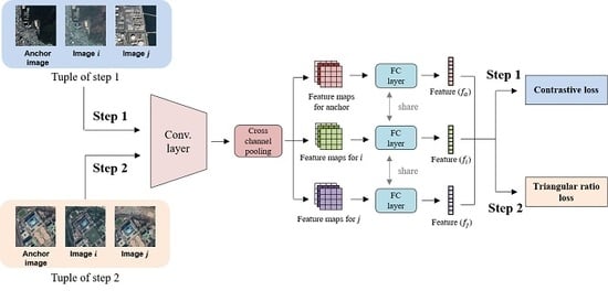
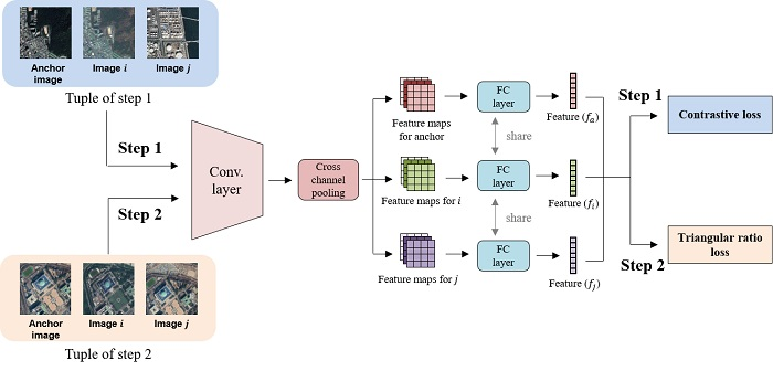
• We propose a coarse-to-fine deep metric learning method for RSIR. In the first step, the network learns the binary relationship and is then retrained to learn the continuous relationship in the second step. The proposed method is end-to-end trainable using the similarity between images.
• We introduce a new loss function to learn continuous information. The triangular ratio loss function considers all the detailed relationships within the tuples, and, therefore, it is appropriate for highly complex RS images that contain many objects.
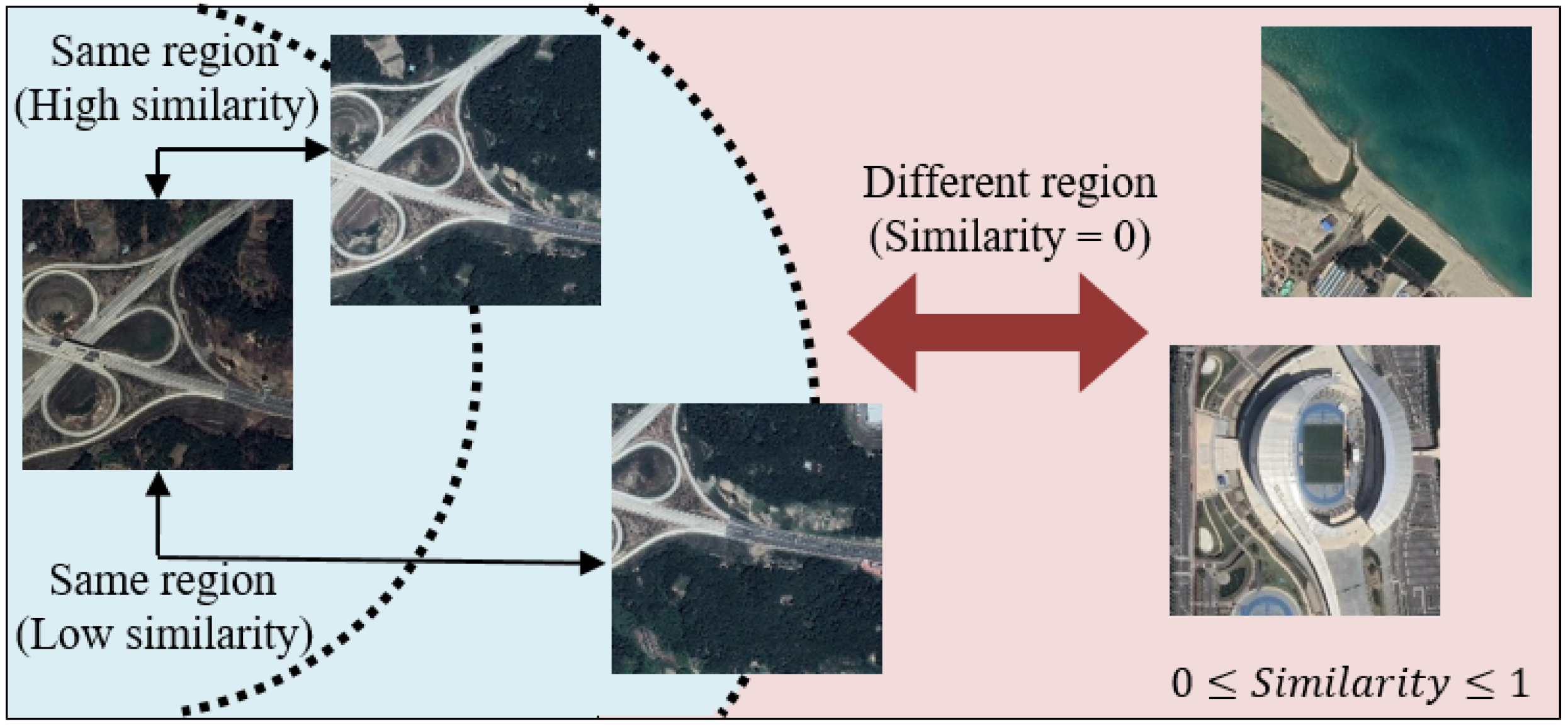
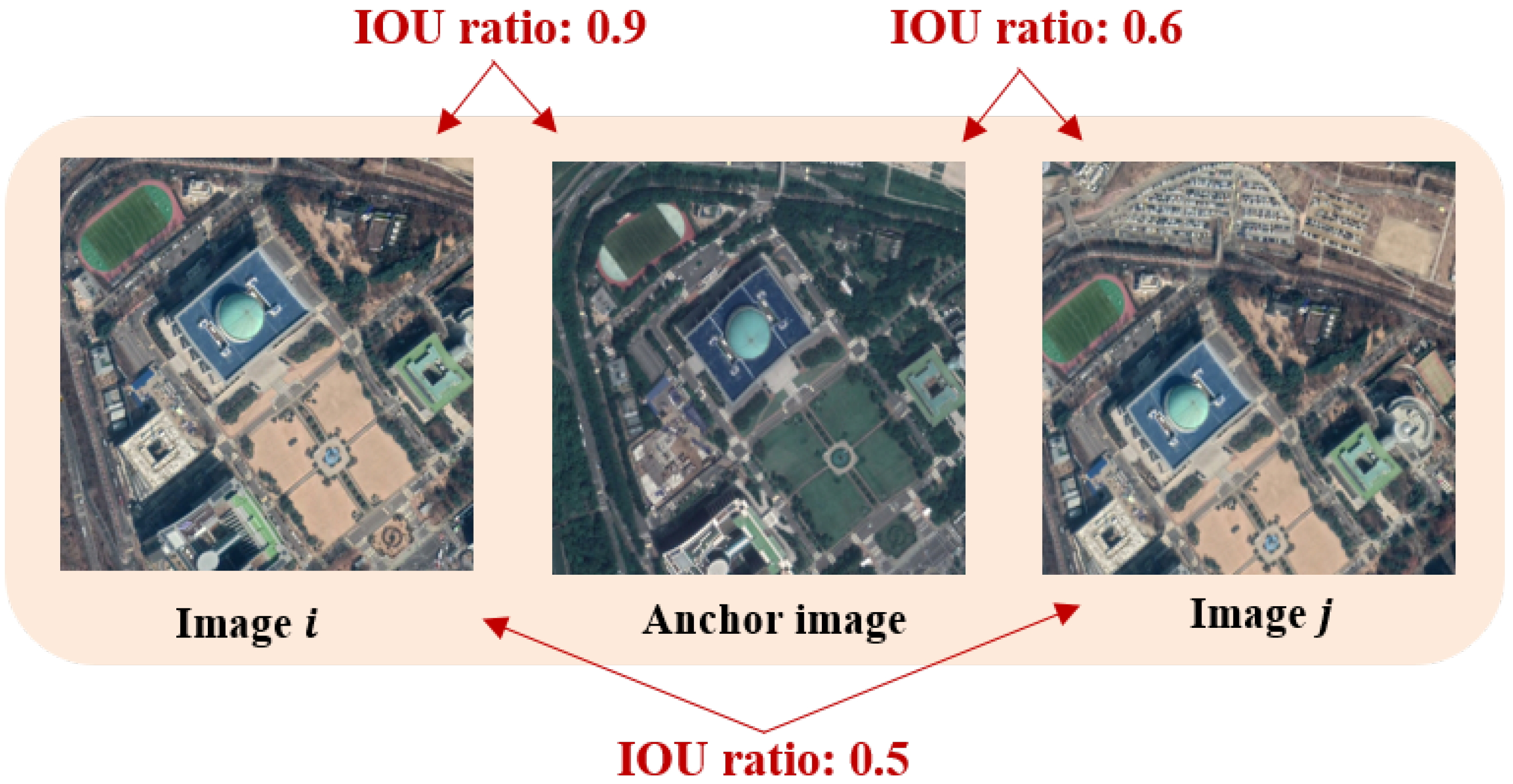
• Using the intersection-over-union (IOU) ratio between images, we confirmed that it is effective to define a continuous similarity between images.

2. Related Work

In general, there are two commonly used deep learning approaches: conventional classification convolutional neural network (CNN) methods [4,7,8,10,44,45] and deep metric learning methods [5,32,39,41,42,43,46,47].

2.1. Image Retrieval for the Conventional CNN Method

Image retrieval using the conventional CNN method is performed as follows [7]: (i) Train the classification task in the conventional CNN structure. (ii) Extract the features from the convolutional layer or fully connected layer of the trained network. The convolutional layer abstracts the image information through window sliding, using shared filter values, and converts it into feature map information. The outputs of the convolutional layer are the feature maps of the image. These feature maps are known to have spatial information and local information about the image. The feature maps are flattened to obtain a set of feature vectors. Let n and m be the number and the size of the feature maps, respectively. The descriptor can be defined as

$$F=[x_1,x_2,x_3,\dots ,x_m],$$

where $x_i(i=1,2,3,\dots ,m)$ is an n-dimensional feature vector. However, the dimension of the feature vector is so large that it is difficult to efficiently summarize it for use in image retrieval. The fully connected layer generates a high-level feature by considering all relationships within the feature summarized through the convolutional layer. The fully connected layer feature is known to lose spatial information and local information because the nodes in the current layer are linked to all nodes in the previous layer. However, the fully connected layer summarizes the entire contents of the image and briefly summarizes the dimensions of the features. Thus, it is effective in summarizing large-capacity images concisely. The feature extractor using fully connected layer is shown in Figure 3.

2.2. Image Retrieval for the Deep Metric Learning Method

The use of the conventional classification CNN method for image retrieval has problems, however. The retrieval process consists of two stages: feature extraction and similarity comparison, as shown in Figure 1. The previous methods do not have these two stages connected. Moreover, the purpose of the training is not for retrieval because only part of the network trained on classification is used as a feature extractor. To overcome these problems, deep metric learning trains the network through the Euclidean distance between features, which is a way to compare the similarity.

Sun et al. [39] proposed the adoption of a metric learning function to a deep network. They trained a deep network through the sample relationship rather than through the class label unit. They utilized a traditional contrastive loss [38] function for the deep network. The authors trained the network by using the relationship between the samples. If two samples had the same attributes, they minimized the Euclidean distance between these samples, and if two samples had different attributes, they maximized the Euclidean distance between these samples. Using this method, they eliminated the need to match the number of nodes in the fully connected layer with the number of labels and solved the suboptimal problem of using only part of the network. Therefore, the contrastive loss function has achieved excellent results in the deep learning field. However, this method does not consider how close/far the samples are to/from each other.

Hoffer and Ailon [42] proposed a triplet loss function. In triplet loss, the distances of same attributes are defined as a positive distance, whereas the distances of different attributes are defined as a negative distance. Using these distances, the function trains the network so that the negative distance is greater than the positive distance in the feature space. Contrastive loss uses the absolute distance of the features, whereas triplet loss uses the relative distance of the features for training. Therefore, in general cases, triplet loss is known to have better performance than that of contrastive loss in the deep learning field. However, defining relationships as binary limits the representation of attributes to just two: they are either the same or different. In addition, network performance varies greatly depending on the sampling methods, and it is difficult to train the network because of the hyperparameter, which is the margin that represents how closely the positive distance will be compared to the negative distance.

As a result, Kim et al. [43] proposed a log ratio loss function that trains the network using continuous relationship. The log ratio loss function defines the similarity between images as a constant value between 0 and 1. Then, the network is trained to learn the ratio of the distance between the features and the defined continuous similarities. Compared with the previous loss function, this function can search for images with more similar content by learning the relationship between images as a continuous variable, and it does not require hyperparameters.

3. Coarse-to-Fine Deep Metric Learning

In this section, we describe a novel network architecture for RSIR. Training is done in two steps using the coarse-to-fine method. In the coarse step, binary information is taught to distinguish the difference of regions. The purpose of this training step is to extract features as similar as possible in identical regions and as different as possible in different regions while ignoring the changes in time instances between the same regions. However, the network will not have the ability to properly distinguish the differences between images of similar regions and identical regions just by this step. Therefore, additional fine learning is necessary to identify the variations of same location regions. In the fine step, the continuous information is learned to realize how much the regions are related. The purpose of this step is to extract features that depend on the similarity of contents between the images. The network is trained according to the change in contents owing to the variation in time instances and parallel shifts of the images with the same region. Once the learning has been completed through these two steps, retrieval can be performed robustly at different time instances or coverage areas between the query image and the database images.

The overall network is used by modifying the last layer using the conventional CNN method. ResNet-34 [30] uses a global average pooling layer to synthesize the channel’s information into the average value of the entire feature map. However, in the case of remote sensing images, spatial information is important, because there are many local features and various objects. Therefore, we applied cross-channel pooling [48] to our network. The illustration of process is shown in Figure 4. Cross-channel pooling is a type of pooling that reduces the dimension of a feature; however, it works differently from conventional maximum pooling and average pooling. Conventional maximum and average pooling methods compress the information within each feature map. They preserve the number of channels but reduce the width and height values of the feature maps. In contrast, cross-channel pooling preserves the width and height values but reduces the number of channels by convolutions of the elements in the same locations of each channel. Through cross-channel pooling, we can reduce the dimension of the features and retain important spatial and local information about the remote sensing images. The fully connected layer consists of an output vector with a dimension of 512, which is the same as that in conventional ResNet-34. Moreover, we used the initial values of the network, which were pretrained on the ImageNet [49] dataset. The overall architecture is shown in Figure 5.

In addition, defining the tuple process is known to be important in metric learning. In the coarse step, we define image i as a location where the longitude and the latitude are exactly the same as those of the anchor image, and we define image j as a different location from that of the anchor image. In the fine step, we create three images so that the IOU region overlap is at least 26% for any two of the three images. Through this process, the network can learn automatically without any human annotation.

3.1. Step 1: Coarse Deep Metric Learning

For training, we constructed data tuples with three images involved. The data tuples consisted of two images from the same region and one from another region. Images from the same region had a time difference of approximately 1 year. The data tuple example of Step 1 is shown in Figure 6. Moreover, the dense triplet mining method [43] was used for efficient learning by organizing images from another region. This method is a way of defining the data tuples for effective metric learning. Using this method, we composed image j, which had the closest Euclidean distance to the anchor image for each mini-batch B.

In Step 1, the network is taught end to end using contrastive loss. Through contrastive loss learning, the network can distinguish information between the regions. As a result, the network extracts more similar features for the same region and more different features for different regions. However, this type of training leads to poor performance when the database image and query images do not have completely identical regions, and additional training must be done to resolve this problem.

Contrastive Loss

Contrastive loss [38,39] is the basic loss function for deep metric learning. This function is appropriate for distinguishing a given pair of images. For training, a data pair ($\{I_i,I_j\}$) is required. The contrastive loss function minimizes the distance in the embedding space when the labels are the same and separates them with a fixed margin when the labels are different. When the contrastive loss training is done, features with the same properties are embedded into the same space, although they have different visual structures. This has been a drawback for other tasks; however, we were able to use it to cope with the variation in content over time that occurred in the same region. The loss function is defined as follows:

$$\mathcal{L}(i,j,y_{i,j})=y_{i,j}D\left(f_i,f_j\right)+(1-y_{i,j}){[m-D\left(f_i,f_j\right)]}_{+}.$$

(1)

Here, $I_i$ and $I_j$ are the image pairs, and $f_i$ and $f_j$ denote the features of each image. y is the indicator of the label. For example, if two images have same label, $y_{i,j}$ becomes 1, and 0 in the other case. ${[*]}_{+}$ is the hinge function, $D(*)$ is the squared Euclidean distance between two features, and m is the margin parameter.

Originally, this loss function was structured to learn about two random data and labels. However, because our data tuple trains three images in units, the loss function was defined as follows:

$$\mathcal{L}(a,i,j)=D\left(f_a,f_i\right)+{[m-D\left(f_a,f_j\right)]}_{+}.$$

(2)

Here, $[I_a,I_i,I_j]$ is an image tuple; and $f_a$, $f_i$, and $f_j$ are the features of each image. ${[*]}_{+}$ is the hinge function, $D(*)$ is a squared Euclidean distance between two features, and m is the margin parameter.

3.2. Step 2: Fine Deep Metric Learning

In the previous step, the network learns the binary relationship that separates the same and different regions. Even if the same area is taken, changes in the shooting range and time instance cause a variation in image contents. Moreover, remote sensing images may have similar contents, even though different regions are captured. With only the first step, the relationship within the region is not learned and the exact regions cannot be retrieved. In addition, the network responds sensitively to small image changes in the same region. To solve this problem, we further train the network to learn the similarity within the region. For the fine step, a tuple with three images is necessary. Three images are extracted from two images of the same area at different times. In each image, one or two crops are performed to obtain three images. The data tuple example of Step 2 is shown in Figure 7. Moreover, the IOU overlaps that measure the amount of common areas between the images are generated. The network is trained through the IOU values obtained.

Triangular Loss

The triangular ratio function was modified according to the log ratio loss function. The log ratio loss function learns the relationship between the anchor and other two images using the continuous label. The log ratio loss function is defined as follows:

$$\begin{array}{cc}\hfill {\mathcal{L}}_{lr}(a,i,j)& ={\{log\frac{D(f_a,f_i)}{D(f_a,f_j)}-log\frac{D(y_a,y_i)}{D(y_a,y_j)}\}}^2.\hfill \end{array}$$

Here, $f_a$ is feature for the anchor image ($I_a$), $f_i$ is the feature for image i ($I_i$), and $f_j$ is the feature for image j ($I_j$). $D(f_{\alpha },f_{\beta })$ is the feature distance (squared Euclidean distance) between two samples ($\alpha ,\beta$). Moreover, $D(y_{\alpha },y_{\beta })$ is a label distance between two samples $(\alpha ,\beta )$.

The log ratio loss function has the advantage of being able to learn the continuous relationship compared with the previous functions that learns the binary relationship. By approximating the ratios between continuous label distances instead of the binary label, the log ratio loss function can learn more accurately in a feature space. Moreover, ideally, the distance between two images in the feature space will be proportional to their label distance. However, because only two of the relationships among the three images were used for training, there was the disadvantage of not considering the relationship between samples i and j.

These problems arise from the consideration of the anchor images. If learning is done in a single step, the definition of the anchor image determines the order of the images being trained. Moreover, the anchor also plays a key role in bridging the relationship between the other two images in this loss function. However, this consideration is not necessary in our coarse-to-fine training. Thus, instead of considering the anchor, we added the relationship between images i and j. We consider when all images become a key factor in the function and modify the formula accordingly. Our triangular ratio loss is defined as follows:

$$\begin{array}{c}\hfill {\mathcal{L}}_{Tgr}(a,i,j)=mean\left\{{\mathcal{L}}_{lr}(a,i,j),{\mathcal{L}}_{lr}(i,a,j),{\mathcal{L}}_{lr}(i,j,a)\right\}.\end{array}$$

Comparing this function to the log ratio function, we observe that the log ratio function directly matches the relationship between a and i to the relationship between a and j. However, our proposed function is taught like the length ratio of a triangle, by considering all relationships in the three images.

The main advantage of the triangular ratio loss function is that it is possible to consider all relationships within the tuple regardless to the order of anchor and other images. The log ratio loss function does not train the relationship between i and j. The proposed loss function trains the relationship from the log ratio loss function and also the relationship between i and j, leading to a more precise embedding. Learning with this function prevents the divergence of the distance between i and j during the continuous learning and results in the gathered images with the same region becoming more closely related to each other.

4. Experiments

4.1. Implementation Details

For the implementation of our network, we utilized the ResNet-34 architecture [30]. We used a pretraining model learned on the ImageNet dataset [49] and fine-tuned the model to extract the features suitable for RSIR. There is no remote sensing image dataset available for searching for identical regions; therefore, we generated training image pairs and retrieval image pairs from the Google Earth South Korea dataset. A detailed description of the data is shown below. The network was end-to-end trained, and all parameters of the network were fine-tuned. In training the fine step, we set a small-enough learning rate because a learning rate that is too big spoils the coarse step. We trained the network for 100 epochs, each with a batch size of 20, which took approximately 2 days on a single GPU (GTX 1080Ti) and CPU (Intel i-7 8700) for each step. As a result, it took an average of 1.7 seconds to retrieve one image. In detail, it is as follows: 1.3 seconds for feature extraction and 0.4 seconds for similarity comparison (for 10,000 database images). Our source code and Google Earth South Korea dataset are online available at https://github.com/sioot.

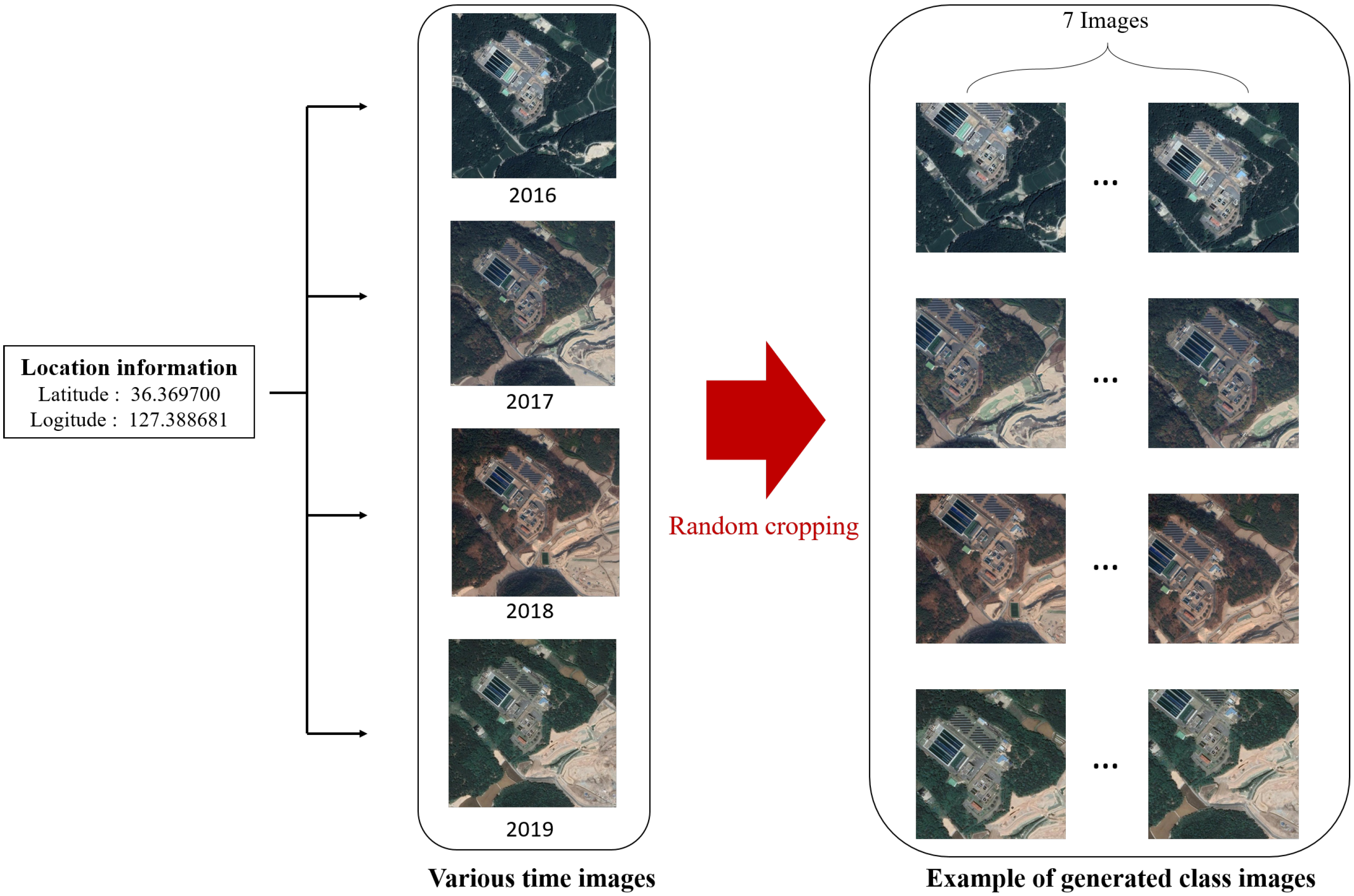
4.2. Google Earth South Korea Dataset

We created a multi-temporal dataset for RSIR using Google Earth [50] images, which were captured by the Landsat 7 and 8 satellites. We acquired three-band (RGB) images from South Korea, excluding the islands. South Korea is a challenging research area because various environmental changes exist, depending on the four seasons, and also because of the existence of various regions, such as cities, mountains, agricultural lands, and the sea. Moreover, the images were geographically registered; however, they were not orthophotos, and, therefore, tall buildings looked different at different time instances. There were also color variations. We divided all satellite images into $1080\times 1080$ images. We gathered satellite images that were taken in 2016, 2017, 2018, and 2019. Each of the four images had the same area but had different time instances. Among the 120,000 images, owing to ambiguity (e.g., mostly composed of sea, cloud, river, and forest), we extracted 40,000 images from them. Figure 8 shows a few examples of these images.

4.3. Experimental Results

To assess our method and experiments, we followed the standard retrieval and place recognition evaluation procedure [9,25,51,52,53]. The query image was deemed to have been correctly retrieved if at least one of the top n retrieved database images overlapped $50\%$ of the contents from the query image. The percentages of correctly retrieved queries (recall) were estimated when $n=1,5,10,$ and 100. The extracted feature dimension was 512. We conducted additional experiments with feature dimensions of 128, 1024, and 3113 for performance evaluations in various dimensions. The feature dimension of 128 had a large drop in performance, whereas feature dimensions greater than 512 were excluded because they did not have any clear improvement in performance.

Quantitative Experiments

We used half of the images for learning (2016 and 2017) and the other half for retrieval (2018 and 2019). We divided the learning set into the training set ($90\%$) and the validation set ($10\%$). In the retrieval set, we used half as a database (2018) and part of the other half as a query image (2019). To select the query images, we randomly sampled 500 different regions. Then, we excluded 111 regions where the contents of the areas were too ordinary to be distinguishable. As a result, image retrieval was conducted with a total of 389 query images. Moreover, the query image consisted of a more than $50\%$ IOU ratio overlapped with the corresponding database image.

• The Conventional Learning Methods
  To add objectivity to our experiments, we used two types of tuples in the conventional methods. Training was done in each of the loss functions. The first type consisted of an anchor image, a positive image with an at least $50\%$ IOU overlap with the anchor image, and a negative image in a different region from that of the anchor image. The first type of tuple was marked with “†” in the

  Table 1. Results of the conventional learning method (with cross-channel pooling) trained on the Google Earth South Korea dataset (Recall@n).

  Methods	$\mathit{Recall}@\mathit{n}(\%)$
  	$n=1$	$n=5$	$n=10$	$n=100$
  Triplet loss †	18.3	23.4	24.7	40.1
  Contrastive loss †	8.7	19.5	25.2	64.5
  Triplet loss	37.8	53.5	59.1	78.4
  Contrastive loss	38.9	55.8	62.7	81.5

  . The second type consisted of an anchor image, a positive image in an exactly identical region as that of the anchor image, and a negative image in a different region from that of the anchor image. We used the transformed triplet loss of Fan et al. [54] for the evaluation of the comparison results, because the basic form has performance degradation problems.
  The results for the first tuple type showed that the overall performance improved for both triplet loss and contrastive losses compared with that of the baseline model. In the detailed comparison of the two loss functions, triplet loss scored $18.3\%$ for r@1, performing better than contrastive loss, which scored $8.7\%$. However, triplet loss scored only $40.1\%$ for r@100, performing worse than contrastive loss, which scored $64.5\%$. For the second tuple type, the overall improvement in performance was greater for contrastive loss than that for triplet loss. Looking into the results for each type of tuples, we observed that the second type showed significantly better performance, because exactly identical regions were matched between images by training with deep metric learning.
  We also conducted an ablation study to see the effects of cross-channel pooling.

  Table 2. Results of the conventional learning (without cross-channel pooling) method trained on the Google Earth South Korea dataset (Recall@n).

  Methods	$\mathit{Recall}@\mathit{n}(\%)$
  	$n=1$	$n=5$	$n=10$	$n=100$
  Baseline network	5.7	11.6	13.9	32.6
  Triplet loss †	4.1	10.5	12.9	25.2
  Contrastive loss †	17.2	35.2	43.7	79.9
  Triplet loss	6.4	10.3	14.4	28.3
  Contrastive loss	30.3	44.2	53.0	81.7

  above shows the performance evaluation results of excluding cross-channel pooling from the method used in Table 1. As a result, most of the loss functions had a noticeable drop in performance. This shows that cross-channel pooling effectively preserves the spatial information, and has a positive effect on the improvement in aerial image retrieval performance.
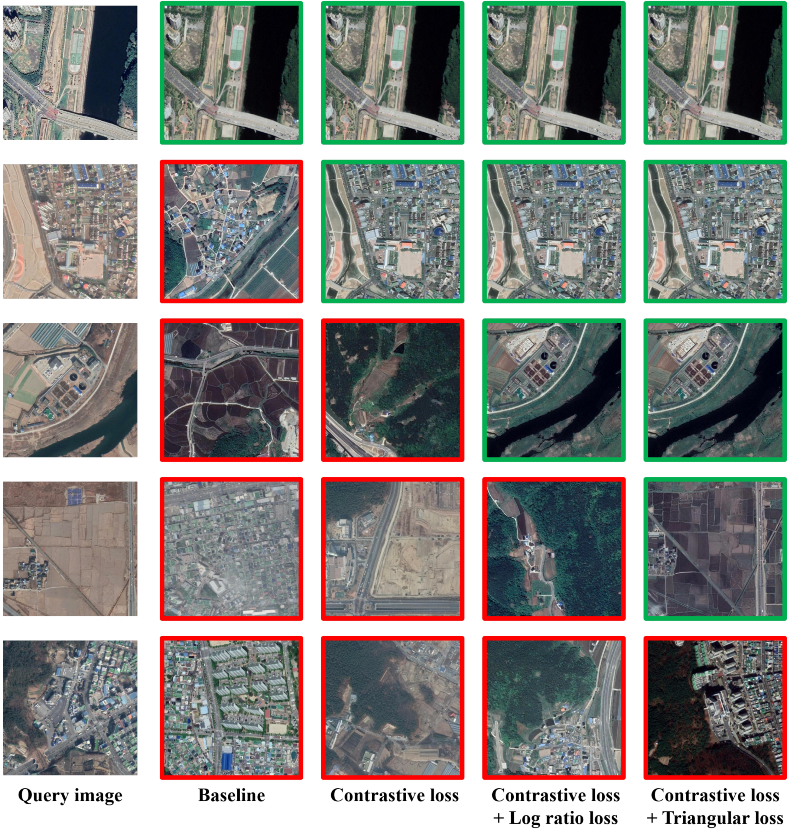
• Coarse-to-Fine Learning Method
  We conducted an experiment by additional learning with the first coarse deep metric learning model. As a result of the coarse deep metric learning, we observed that using the second type of tuple that defined the positive image as an image in the exact same region as that of the anchor image led to better performance.
  The

  Table 3. Result of the coarse-to-fine learning method trained on the Google Earth South Korea dataset (Recall@n).

  Methods		$\mathit{Recall}@\mathit{n}(\%)$
  Step 1	Step 2	$n=1$	$n=5$	$n=10$	$n=100$
  Triplet loss	Log ratio loss	44.2	57.8	2.0	78.7
  Triplet loss	Triangular loss	46.8	59.4	65.8	82.5
  Contrastive loss	Log ratio loss	47.6	61.4	66.8	86.7
  Contrastive loss	Triangular loss	49.1	62.5	67.1	87.1

  shows the retrieval result using the coarse-to-fine method. We can confirm the effectiveness of the coarse-to-fine training. Performance improved in the triplet-loss-based model and in the contrastive-loss-based model.
  The performance improved more for the former model than that for the latter model. Triplet loss forces the distance between the anchor and the positive to be smaller than that between the anchor and the negative. Contrastive loss maximizes the distance between the anchor and the negative, while minimizing the distance between the anchor and the positive. Therefore, contrastive loss identifies the distance between features more strictly than the triplet loss. In addition, it was shown that coarse-to-fine learning resulted in better performance when trained with strictly defined features. Moreover, the overall performance showed greater improvement when using triangular loss than when using log ratio loss. Figure 9. shows examples of the coarse model and coarse-to-fine model retrieval results based on contrastive loss with the best performance.
  We integrated the steps of the method proposed in

  Table 4. Results of the conventional learning method trained on the Google Earth South Korea dataset (Recall@n).

  Methods	$\mathit{Recall}@\mathit{n}(\%)$
  	$n=1$	$n=5$	$n=10$	$n=100$
  Integrated method	33.6	44.7	49.4	70.4
  Coarse-to-Fine method	49.1	62.5	67.1	87.1

  and evaluated the performance after training. The overall recall performance degradation occurred when the training was conducted in integration. This shows that the proposed two-step approach is more effective than the integrated approach.
• Comparison with State-Of-The-Art
  As shown in the

  Table 5. Comparisions of retrieval result with state-of-the-art methods on the Google Earth South Korea dataset (Recall@n).

  Methods	$\mathit{Recall}@\mathit{n}(\%)$
  	$n=1$	$n=5$	$n=10$	$n=100$
  LDCNN	8.2	15.6	19.2	39.3
  R-MAC descriptor	15.9	24.7	30.6	48.8
  NetVlad	16.2	27.8	33.7	55.0
  Triplet loss	37.8	53.5	59.1	78.4
  Constrastive loss	38.9	55.8	62.7	81.5
  Coarse-to-Fine method	49.1	62.5	67.1	87.1

  , we compared various SOTA methods in the field of image retrieval with our coarse to fine method. The models used for comparison were LDCNN [7], R-MAC Descriptor [45], NetVlad [51], triplet loss, and contrastive loss. These methods are widely used in image retrieval. LDCNN is a method of using low-level features of CNN through the mlpconv layers. R-MAC method identifies the activations of the convolutional feature maps, and uses the features of the parts determined to be important. LDCNN and R-MAC are classification-oriented methods, and therefore, a classification-labeled dataset is needed to train these two models. We used the AID dataset with features (altitude, picture quality, etc.) most similar to the Google Earth South Korea dataset. NetVlad method is primarily used in a smartphone environment for GPS location image retrieval. The method is robust to light changes and obscuring objects. NetVlad method was used with the same conditions as those used for coarse learning, and dense triplet mining was used for the sampling method. The backbone network used for the comparison methods was ResNet-34, except for LDCNN, which used the VGG-16 [34] network because of the number of parameters. As a result, the LDCNN used 490 dimensional feature vectors and the other models used 512 dimensional feature vectors. We confirm that the coarse to fine method has a noticeable difference compared to other SOTA methods.

4.4. Feature Analysis

4.4.1. Visualization of the Feature Descriptor

We observed the feature distributions of the query image that corresponded to those of the database image. The database image and the query image shared the same location. However, the two images had field variations due to the differences in time instances and had content-wise variation due to the shooting range of the images. The network must recognize these two images as identical to successfully retrieve under these circumstances. To observe how the baseline network and the network trained by the proposed method interpreted the two images, we visualized the feature descriptors. Of the 512 feature dimensions of each network, we plotted for every multiple of four. As shown in Figure 10, the baseline network feature descriptors have fewer overlaps for the two images, whereas the proposed network feature descriptor has, relatively, a lot of overlaps. This comparatively shows that the proposed network recognizes the two images as identical regions.

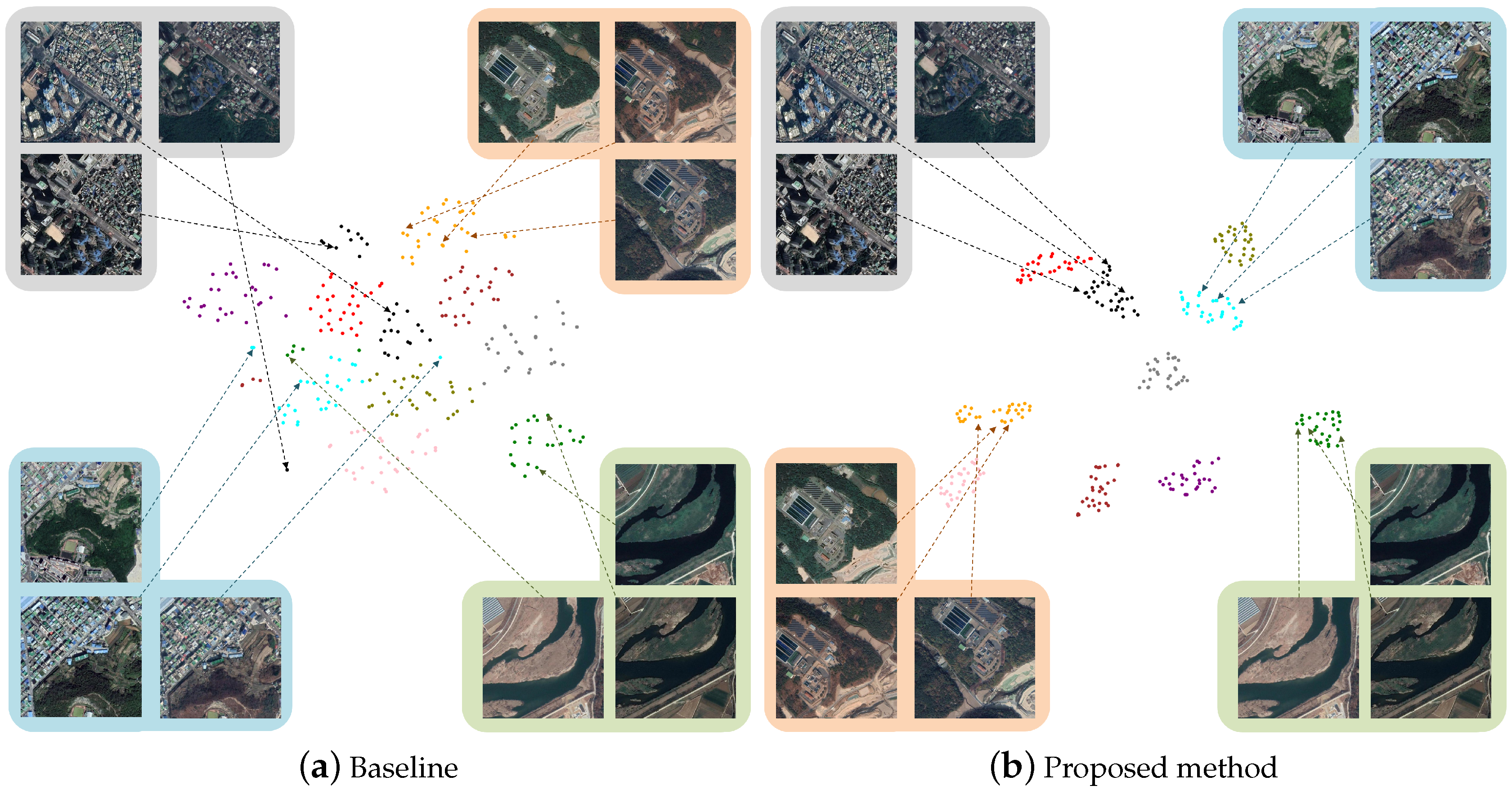
4.4.2. Location Wise t-SNE

To investigate the embedding distribution of our trained network, we performed an additional analysis on the Google Earth South Korea dataset. First, we selected 10 different regions from the said dataset. Then, we selected different times (2016, 2017, 2018, and 2019) and different scopes ($0.26\le IOU\le 1$) of those regions for intraregional variation, as shown in Figure 11.

Figure 12 shows the t-distributed stochastic neighbor embedding (t-SNE) distributions for 10 different regions of the baseline model and the proposed model. Each of the 10 different regions is represented in 10 different colors, and the 512 feature dimensions are visualized in two dimensions through the t-SNE method. The baseline model t-SNE result is shown in Figure 12a. The baseline model often extracted different features for the same region, depending on the time instance and the shooting range of the images. In particular, if the green field is included in the image, the gray-colored class is considered to be closer to the sky blue-colored class. Moreover, the green-colored class cannot be clustered or categorized properly within the t-SNE distribution because of the overall change in color of the images by the variation in time instance. However, training done with the proposed model shows regionally distinct distributions of the images in the t-SNE distribution despite the variations in time instance and shooting range. The baseline model t-SNE result is shown in Figure 12b.

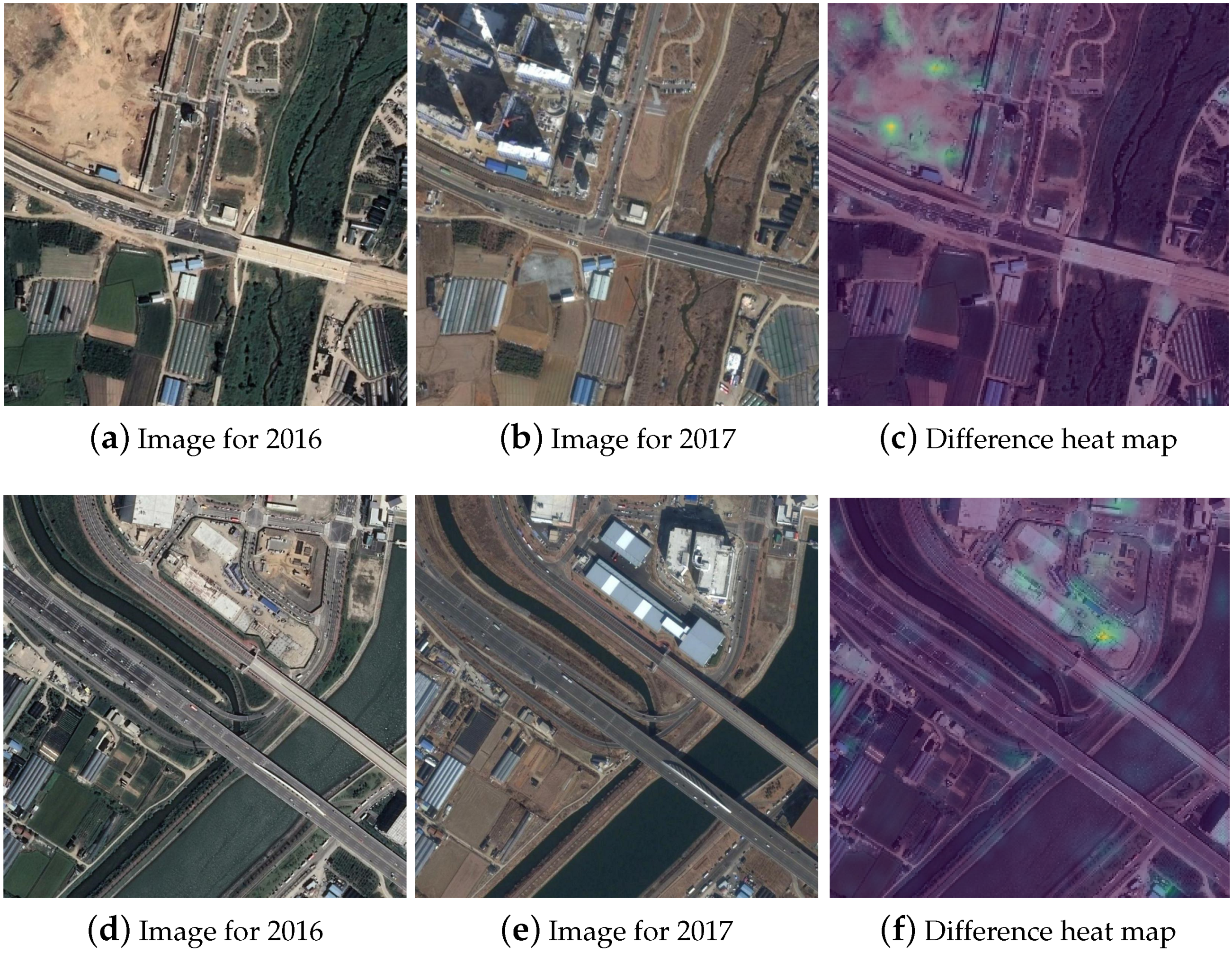
4.4.3. Recognition of Differences Between Images

We conducted an experiment to determine what the proposed network considers as an important difference. Looking into the Figure 13, the difference heat map is shown. For each row, the two images on the left are input images and two images on the right are what the network considers as the difference. In the heat map is shown by calculating the squared difference between the convolutional layer feature maps. Because the network was trained to determine the differences in time variation, it did not consider field color and vehicle changes as differences because they were natural changes. However, important information changes, such as new buildings, were considered pivotal differences.

5. Discussion

We used the Google Earth South Korea dataset to confirm the effectiveness of coarse-to-fine learning and the proposed loss function. In the quantitative result, coarse-to-fine learning models showed better performance than that of the single (coarse) learning method. The proposed model showed the best performance among the models. Comparing the two types of loss functions used for the coarse method, we observed that contrastive loss showed better performance than that of triplet loss. The model that used contrastive loss function showed the best performance, with a score of $49.1\%$ for r@1 on the Google Earth South Korea dataset. We conducted three qualitative assessments to further analyze our trained network. For the first assessment, we compared the trained network and the baseline network by visualizing the feature descriptors. As a result, the trained network extracted relatively similar features for identical regions that had different time instances and parallel shifts. For the second assessment, we selected 10 locations and four different time instances from the Google Earth South Korea dataset and made variations in the shooting range to visualize the distribution of the features. From the t-SNE figure, it is shown that identical regions with different time instances were recognized as relatively similar to each other. Finally, we analyzed what the trained model recognized as the differences between the two images with different time instances but with identical regions. The analysis process used the differences between features in the convolutional layer to observe what the network recognized as the differences between the images. Natural changes, such as changes in grasslands and the presence of cars, were ignored, and major changes, such as the presence of buildings, were recognized as differences.

6. Conclusions

We proposed a novel method based on end-to-end trainable deep metric learning for remote sensing image retrieval. The proposed method is designed to train by using a coarse-to-fine strategy. In the coarse step, the images are differentiated in a binary manner and trained. In the fine step, features are extracted depending on the overlap of contents between images using continuous values.

Furthermore, our network is end-to-end trainable using the similarity between images. Moreover, we proposed a new loss function for deep metric learning. This function is more precisely teachable than the previous methods because it reflects the entire triple relationship. As a result, our method can cope with a change in both time instance and shooting range between the database image and the query image. Experimental result shows that the proposed coarse-to-fine method improved performance compared to other methods on the Google Earth South Korea dataset.

In this study, we dealt with the variation in time instance and shooting range of the image. However, to use the proposed method widely, we should consider the rotational or torsional transformations. We plan to extend this method to deal with these transformations in the future.

References

1. Cheng, G.; Yang, C.; Yao, X.; Guo, L.; Han, J. When deep learning meets metric learning: Remote sensing image scene classification via learning discriminative CNNs. IEEE Trans. Geosci. Remote. Sens. 2018, 56, 2811–2821. [Google Scholar] [CrossRef]
2. Mahdianpari, M.; Salehi, B.; Rezaee, M.; Mohammadimanesh, F.; Zhang, Y. Very deep convolutional neural networks for complex land cover mapping using multispectral remote sensing imagery. Remote. Sens. 2018, 10, 1119. [Google Scholar] [CrossRef] [Green Version]
3. Zhu, X.X.; Tuia, D.; Mou, L.; Xia, G.-S.; Zhang, L.; Xu, F.; Fraundorfer, F. Deep learning in remote sensing: A comprehensive review and list of resources. IEEE Geosci. Remote. Sens. Mag. 2017, 5, 8–36. [Google Scholar] [CrossRef] [Green Version]
4. Xiong, W.; Lv, Y.; Cui, Y.; Zhang, X.; Gu, X. A discriminative feature learning approach for remote sensing image retrieval. Remote. Sens. 2019, 11, 281. [Google Scholar] [CrossRef] [Green Version]
5. Cao, R.; Zhang, Q.; Zhu, J.; Li, Q.; Li, Q.; Liu, B.; Qiu, G. Enhancing remote sensing image retrieval with triplet deep metric learning network. arXiv 2019, arXiv:1902.05818. [Google Scholar] [CrossRef] [Green Version]
6. Zhou, W.; Deng, X.; Shao, Z. Region convolutional features for multi-label remote sensing image retrieval. arXiv 2018, arXiv:1807.08634. [Google Scholar]
7. Zhou, W.; Newsam, S.; Li, C.; Shao, Z. Learning low dimensional convolutional neural networks for high-resolution remote sensing image retrieval. Remote. Sens. 2017, 9, 489. [Google Scholar] [CrossRef] [Green Version]
8. Yue-Hei Ng, J.; Yang, F.; Davis, L.S. Exploiting local features from deep networks for image retrieval. In Proceedings of the IEEE Conference on Computer vision and Pattern Recognition Workshops, Santiago, Chile, 7–13 December 2015; pp. 53–61. [Google Scholar]
9. Sattler, T.; Weyand, T.; Leibe, B.; Kobbelt, L. Image retrieval for image-based localization revisited. In Proceedings of the British Machine Vision Conference, Surrey, UK, 3–7 September 2012; p. 4. [Google Scholar]
10. Wan, J.; Wang, D.; Hoi, S.C.H.; Wu, P.; Zhu, J.; Zhang, Y.; Li, J. Deep learning for content-based image retrieval: A comprehensive study. In Proceedings of the 22nd ACM International Conference on Multimedia, Orlando, FL, USA, 3–7 November 2014; pp. 157–166. [Google Scholar]
11. Maeng, H.; Liao, S.; Kang, D.; Lee, S.-W.; Jain, A.K. Nighttime face recognition at long distance: Cross-distance and cross-spectral matching. In Proceedings of the 11th Asian Conference on Computer Vision, Daejeon, Korea, 5–9 November 2012; pp. 708–721. [Google Scholar]
12. Park, S.-C.; Lim, S.-H.; Sin, B.-K.; Lee, S.-W. Tracking non-rigid objects using probabilistic Hausdorff distance matching. Pattern Recognit. 2005, 38, 2373–2384. [Google Scholar] [CrossRef]
13. Park, S.-C.; Lee, H.-S.; Lee, S.-W. Qualitative estimation of camera motion parameters from the linear composition of optical flow. Pattern Recognit. 2004, 37, 767–779. [Google Scholar] [CrossRef]
14. Roh, H.-K.; Lee, S.-W. Multiple people tracking using an appearance model based on temporal color. In Proceedings of the International Workshop on Biologically Motivated Computer Vision, Seoul, Korea, 15–17 May 2000; pp. 369–378. [Google Scholar]
15. Park, J.; Kim, H.-Y.; Park, Y.; Lee, S.-W. A synthesis procedure for associative memories based on space-varying cellular neural networks. Neural Netw. 2001, 14, 107–113. [Google Scholar] [CrossRef]
16. Roh, M.-C.; Kim, T.-Y.; Park, J.; Lee, S.-W. Accurate object contour tracking based on boundary edge selection. Pattern Recognit. 2007, 40, 931–943. [Google Scholar] [CrossRef]
17. Xi, D.; Podolak, I.T.; Lee, S.-W. Facial component extraction and face recognition with support vector machines. In Proceedings of the Fifth IEEE International Conference on Automatic Face Gesture Recognition, Guildford, UK, 9–11 June 2003; pp. 83–88. [Google Scholar]
18. Suk, H.-I.; Sin, B.-K.; Lee, S.-W. Recognizing hand gestures using dynamic bayesian network. In Proceedings of the 2008 8th IEEE International Conference on Automatic Face & Gesture Recognit, Amsterdam, The Netherlands, 17–19 September 2008; pp. 1–6. [Google Scholar]
19. Roh, M.-C.; Shin, H.-K.; Lee, S.-W. View-independent human action recognition with volume motion template on single stereo camera. Pattern Recognit. Lett. 2010, 31, 639–647. [Google Scholar] [CrossRef]
20. Park, U.; Choi, H.-C.; Jain, A.K.; Lee, S.-W. Face tracking and recognition at a distance: A coaxial and concentric PTZ camera system. IEEE Trans. Inf. Forensics Secur. 2013, 8, 1665–1677. [Google Scholar] [CrossRef]
21. Jung, H.-C.; Hwang, B.-W.; Lee, S.-W. Authenticating corrupted face image based on noise model. In Proceedings of the Sixth IEEE International Conference on Automatic Face and Gesture Recognition, Hong Kong, China, 15–17 July 2004; pp. 272–277. [Google Scholar]
22. Hwang, B.-W.; Blanz, V.; Vetter, T.; Lee, S.-W. Face reconstruction from a small number of feature points. In Proceedings of the 15th International Conference on Pattern Recognition, Seoul, Korea, 15–17 May 2000; pp. 838–841. [Google Scholar]
23. Song, H.-H.; Lee, S.-W. LVQ combined with simulated annealing for optimal design of large-set reference models. Neural Netw. 1996, 9, 329–336. [Google Scholar] [CrossRef]
24. Suk, H.-I.; Jain, A.K.; Lee, S.-W. A network of dynamic probabilistic models for human interaction analysis. IEEE Trans. Circuits Syst. Video Technol. 2011, 21, 932–945. [Google Scholar]
25. Thrun, S.; Zlot, R. Reduced sift features for image retrieval and indoor localization. In Proceedings of the Australian Conference on Robotics and Automation, Canberra, Australia, 6–8 December 2004; pp. 1–8. [Google Scholar]
26. Lowe, D.G. Distinctive image features from scale-invariant keypoints. Int. J. Comput. Vis. 2004, 60, 91–110. [Google Scholar] [CrossRef]
27. Pass, G.; Zabih, R. Histogram refinement for content-based image retrieval. In Proceedings of the Third IEEE Workshop on Applications of Computer Vision, Sarasota, FL, USA, 2–4 December 1996; pp. 96–102. [Google Scholar]
28. Aptoula, E. Remote sensing image retrieval with global morphological texture descriptors. IEEE Trans. Geosci. Remote. Sens. 2013, 52, 3023–3034. [Google Scholar] [CrossRef]
29. He, K.; Gkioxari, G.; Dollár, P.; Girshick, R. Mask r-cnn. In Proceedings of the IEEE Conference on Computer Vision and Pattern Recognition, Honolulu, HI, USA, 21–26 July 2017; pp. 5620–5629. [Google Scholar]
30. He, K.; Zhang, X.; Ren, S.; Sun, J. Deep residual learning for image recognition. In Proceedings of the IEEE Conference on Computer Vision and Pattern Recognition, Las Vegas, NV, USA, 26 June–1 July 2016; pp. 770–778. [Google Scholar]
31. Ren, S.; He, K.; Girshick, R.; Sun, J. Faster r-cnn: Towards real-time object detection with region proposal networks. In Proceedings of the Advances in Neural Information Processing Systems, Montreal, QC, Canada, 7–12 December 2015; pp. 91–99. [Google Scholar]
32. Son, J.; Baek, M.; Cho, M.; Han, B. Multi-object tracking with quadruplet convolutional neural networks. In Proceedings of the IEEE Conference on Computer Vision and Pattern Recognition, Honolulu, HI, USA, 21–26 July 2017; pp. 5620–5629. [Google Scholar]
33. Zheng, L.; Yang, Y.; Tian, Q. SIFT meets CNN: A decade survey of instance retrieval. IEEE Trans. Pattern Anal. Mach. Intell. 2017, 40, 1224–1244. [Google Scholar] [CrossRef] [Green Version]
34. Simonyan, K.; Zisserman, A. Very deep convolutional networks for large-scale image recognition. arXiv 2014, arXiv:1409.1556. [Google Scholar]
35. Yang, Y.; Newsam, S. Bag-of-visual-words and spatial extensions for land-use classification. In Proceedings of the 18th SIGSPATIAL International Conference on Advances in Geographic Information Systems, San Jose, CA, USA, 2–5 November 2010; pp. 270–279. [Google Scholar]
36. Xia, G.-S.; Hu, J.; Hu, F.; Shi, B.; Bai, X.; Zhong, Y.; Zhang, L.; Lu, X. AID: A benchmark data set for performance evaluation of aerial scene classification. IEEE Trans. Geosci. Remote. Sens. 2017, 55, 3965–3981. [Google Scholar] [CrossRef] [Green Version]
37. Sun, B.; Chen, C.; Zhu, Y.; Jiang, J. GeoCapsNet: Aerial to Ground view Image Geo-localization using Capsule Network. arXiv 2019, arXiv:1904.06281. [Google Scholar]
38. Chopra, S.; Hadsell, R.; LeCun, Y. Learning a similarity metric discriminatively, with application to face verification. In Proceedings of the IEEE Conference on Computer Vision and Pattern Recognition, San Diego, CA, USA, 20–26 June 2005; pp. 907–914. [Google Scholar]
39. Sun, Y.; Chen, Y.; Wang, X.; Tang, X. Deep learning face representation by joint identification-verification. In Proceedings of the Advances in Neural Information Processing Systems, Montreal, QC, Canada, 8–13 December 2014; pp. 1988–1996. [Google Scholar]
40. Kumar, B.; Carneiro, G.; Reid, I. Learning local image descriptors with deep siamese and triplet convolutional networks by minimising global loss functions. In Proceedings of the IEEE Conference on Computer Vision and Pattern Recognition, Las Vegas, NV, USA, 26 June–1 July 2016; pp. 5385–5394. [Google Scholar]
41. Schroff, F.; Kalenichenko, D.; Philbin, J. Facenet: A unified embedding for face recognition and clustering. In Proceedings of the IEEE Conference on Computer Vision and Pattern Recognition, Santiago, Chile, 7–13 December 2015; pp. 815–823. [Google Scholar]
42. Hoffer, E.; Ailon, N. Deep metric learning using triplet network. In Proceedings of the International Workshop on Similarity-Based Pattern Recognition, Copenhagen, Denmark, 12–14 October 2015; pp. 84–92. [Google Scholar]
43. Kim, S.; Seo, M.; Laptev, I.; Cho, M.; Kwak, S. Deep Metric Learning Beyond Binary Supervision. In Proceedings of the IEEE Conference on Computer Vision and Pattern Recognition, Long Beach, CA, USA, 16–20 June 2019; pp. 2288–2297. [Google Scholar]
44. Babenko, A.; Lempitsky, V. Aggregating local deep features for image retrieval. In Proceedings of the IEEE Conference on Computer Vision and Pattern Recognition, Santiago, Chile, 7–13 December 2015; pp. 1269–1277. [Google Scholar]
45. Tolias, G.; Sicre, R.; Jégou, H. Particular object retrieval with integral max-pooling of CNN activations. arXiv 2015, arXiv:1511.05879. [Google Scholar]
46. Chen, W.; Chen, X.; Zhang, J.; Huang, K. Beyond triplet loss: a deep quadruplet network for person re-identification. In Proceedings of the IEEE Conference on Computer Vision and Pattern Recognition, Honolulu, HI, USA, 21–26 July 2017; pp. 403–412. [Google Scholar]
47. Sohn, K. Improved deep metric learning with multi-class n-pair loss objective. In Proceedings of the Advances in Neural Information Processing Systems, Barcelona, Spain, 5–10 December 2016; pp. 1857–1865. [Google Scholar]
48. Liu, L.; Shen, C.; Van Den Hengel, A. Cross-convolutional-layer pooling for image recognition. IEEE Trans. Geosci. Remote. Sens. 2016, 39, 2305–2313. [Google Scholar] [CrossRef] [PubMed] [Green Version]
49. Deng, J.; Dong, W.; Socher, R.; Li, L.-J.; Li, K.; Fei-Fei, L. Imagenet: A large-scale hierarchical image database. In Proceedings of the IEEE Conference on Computer Vision and Pattern Recognition, Miami, FL, USA, 20–25 June 2009; pp. 248–255. [Google Scholar]
50. Gorelick, N.; Hancher, M.; Dixon, M.; Ilyushchenko, S.; Thau, D.; Moore, R. Google Earth Engine: Planetary-scale geospatial analysis for everyone. Remote. Sens. Environ. 2017, 202, 18–27. [Google Scholar] [CrossRef]
51. Arandjelovic, R.; Gronat, P.; Torii, A.; Pajdla, T.; Sivic, J. NetVLAD: CNN architecture for weakly supervised place recognition. In Proceedings of the IEEE Conference on Computer Vision and Pattern Recognition, Las Vegas, NV, USA, 26 June–1 July 2016; pp. 5297–5307. [Google Scholar]
52. Torii, A.; Sivic, J.; Pajdla, T.; Okutomi, M. Visual place recognition with repetitive structures. In Proceedings of the IEEE Conference on Computer Vision and Pattern Recognition, Portland, OR, USA, 25–27 June 2013; pp. 883–890. [Google Scholar]
53. Gronat, P.; Obozinski, G.; Sivic, J.; Pajdla, T. Learning and calibrating per-location classifiers for visual place recognition. In Proceedings of the IEEE Conference on Computer Vision and Pattern Recognition, Portland, OR, USA, 23–28 June 2013; pp. 907–914. [Google Scholar]
54. Fan, C.; Lee, J.; Xu, M.; Kumar Singh, K.; Jae Lee, Y.; Crandall, D.J.; Ryoo, M.S. Identifying first-person camera wearers in third-person videos. In Proceedings of the IEEE Conference on Computer Vision and Pattern Recognition, Honolulu, HI, USA, 21–26 July 2017; pp. 5125–5133. [Google Scholar]
Figure 1. Illustration of the remote sensing image retrieval process. Features are extracted from database and query image, and the Euclidean distance between them is calculated to determine the priority. Images are retrieved in order based on the minimum Euclidean distance.
Remotesensing 12 00219 g001
Figure 2. Illustration of the feature embedding concept. First, the regions between images are distinguished in a binary manner, which denotes the same region or not. Then, the degree of similarity is defined as a label, which indicates how the contents of the images overlap each other. The distance of the features is rearranged according to the similarity.
Remotesensing 12 00219 g002
Figure 3. Overview of the conventional CNN architecture used in image retrieval. The network is trained to classify labels with learning high-level features of the contents. Those features are then utilized to retrieve the images.
Remotesensing 12 00219 g003
Figure 4. Illustration of the cross-channel pooling process. The pooling operation is done using the elements in the same location of each feature map. As a result, the width (w) and height (h) of the feature maps are preserved while reducing the dimensions of the channel (c).
Remotesensing 12 00219 g004
Figure 5. Overall architecture of the proposed training step. There are two streams: (i) Training with the contrastive loss function using Step 1 tuples, which contain two same images and one different image. (ii) Retraining with the triangular loss function using Step 2 tuples, which consist of three same region images.
Remotesensing 12 00219 g005
Figure 6. Data tuple example of Step 1. The data tuples consist of the anchor image, image i, and image j. Image i is taken from the same area of the anchor image, and image j is taken from different areas of the anchor image.
Remotesensing 12 00219 g006
Figure 7. Data tuple example of Step 2. The data tuples consist of the anchor image, image i, and image j. All images were taken from the same area but had different variables during capture.
Remotesensing 12 00219 g007
Figure 8. Sample images from the Google Earth South Korea dataset. The photographs were taken in (a,e,i) 2016, (b,f,j) 2017, (c,g,k) 2018, and (d,h,l) 2019.
Remotesensing 12 00219 g008
Figure 9. Examples of the retrieval results on the Google Earth South Korea dataset. Each row corresponds to one test case: the query is shown in the first column, the baseline in the second column, the coarse model in the third column, and the coarse-to-fine models in the fourth and fifth columns. Our trained network shows relatively stable retrieval results despite the variations in time instance and shooting range.
Remotesensing 12 00219 g009
Figure 10. Visualization feature descriptors on the matching patch pairs of the database image and the query images. The two pictures on top were the database image and the corresponding query image, respectively. The graph in the second row shows the feature of the two images using the baseline model. The graph in the third row shows the features of the proposed coarse-to-fine trained network.
Remotesensing 12 00219 g010
Figure 11. Illustration of the process of generating class images.
Remotesensing 12 00219 g011
Figure 12. t-SNE figure before and after learning.
Remotesensing 12 00219 g012
Figure 13. Heat maps representing the differences in features between images.
Remotesensing 12 00219 g013