Spatial Heterogeneity of Vegetation Response to Mining Activities in Resource Regions of Northwestern China

Abstract

Aggregated mining development has direct and indirect impacts on vegetation changes. This impact shows spatial differences due to the complex influence of multiple mines, which is a common issue in resource regions. To estimate the spatial heterogeneity of vegetation response to mining activities, we coupled vegetation changes and mining development through a geographically weighted regression (GWR) model for three cumulative periods between 1999 and 2018 in integrated resource regions of northwestern China. Vegetation changes were monitored by Sen’s slope and the Mann–Kendall test according to a total of 72 Landsat images. Spatial distribution of mining development was quantified, due to four land-use maps in 2000, 2005, 2010, and 2017. The results showed that 80% of vegetation in the study area experienced different degrees of degradation, more serious in the overlapping areas of multiple mines and mining areas. The scope of influence for single mines on vegetation shrunk by about 48%, and the mean coefficients increased by 20%, closer to mining areas. The scope of influence for multiple mines on vegetation gradually expanded to 86% from the outer edge to the inner overlapping areas of mining areas, where the mean coefficients increased by 92%. The correlation between elevation and vegetation changes varied according to the average elevation of the total mining areas. Ultimately, the available ecological remediation should be systematically considered for local conditions and mining consequences.

1. Introduction

Vegetation dominating terrestrial ecosystems connects the material circulation and energy flow of the biosphere [1] and plays a critical role in supporting ecosystem services and functions [2,3]. Vegetation changes, thus, have increasingly become an inevitable indicator in global climate changes and regional eco-environmental assessment [4,5]. Changes in natural conditions and strong human activities involve ecological elements and ecological processes, and alter the regional environment [6]. As intensive human activities, mining activities have an impact on 11 out of the 17 United Nations Sustainable Development Goals (SDGs) [7], and are a constraint for achieving sustainable development [8]. Mining activities, especially extractive ones, directly destroy vegetation and indirectly lead to environmental problems, including air and water pollution [9], heavy-metal pollution [10], groundwater loss [11], soil erosion and degradation [12]. These problems profoundly change the environment of vegetation growth, and, in turn, disproportionately damage broader range of vegetation coverages and show spatial differences on vegetation changes. The vegetation changes representing local ecosystem health are severely disturbed by mining activities [13]. Research on the effect of mining activities on vegetation is essential for further ecological construction and achieving the SDGs.

Analyzing the mechanism of mining activities on vegetation growth in mining areas provides significant insight for constructing ecological coal mining [14]. Researchers have made many findings through field surveys and experiments focusing on soil parameters [15], microorganisms [16], root environments [17], toxicological effects [18,19], colony symbiosis and photosynthesis [20], heavy-metal pollution and enrichment in vegetation [21,22], the extinction of major dominant species [23], and biodiversity loss [24]. Related studies have revealed that mining approaches impacting vegetation growth are diversiform on a local scale and more complicated on a regional scale [25]. However, mining development in resource regions is not a single sporadic mine pit, but a complex and systematic industrial chain [26]. This chain involves a wholly integrated process and establishes diversified industrial branches from mining excavation, transportation, preprocessing, and deep processing, to material consumption and utilization [26,27]. The successive impacts are constantly accumulated by the aggregation of one or more activities on receptors [28,29]. The difference in the spatial accumulation degree over time and space causes different responses of various vegetation types to mining development on a regional scale, resulting in significant spatial heterogeneity. Understanding how mining impacts accumulate, and change over time is the key issue for assessing and monitoring vegetation response to mining activities.

The regional ecological impact of mining development could be revealed through large-scale observation [30]. Recent achievements include that coal mining is an important driving factor resulting in serious regional vegetation degradation, especially in China’s Mongolia Plateau and alpine areas [29,30,31]. Vegetation disturbance caused by mining is evident on a large scale [30], and much more significant in arid and semiarid areas [25,31]. The combined effect of climate conditions and ecological restoration activities also make vegetation changes more volatile and show vast spatial differences [30,32]. In relation to the regional scale, the relationship between mining development and vegetation changes during the aggregation progress of mining development and the typical region where mining activities influence more significantly, are still not well-understood. Establishing a mathematical coupling model between vegetation trends and human activities is essential in a complex system under the coupling of natural conditions and human activities [33].

Spatial analysis provides an advantage in understanding the variation in the impact of mining on vegetation [34]. Traditional multivariate statistical analysis and simple spatial analysis, such as ordinary least squares (OLS) models, usually assume that spatial relationships between variables are stable in the entire study area and reflect any variation of spatial characteristics with difficulty [35]. Geographically weighted regression (GWR) constructs local regression equations from any given geographic location to represent accurate quantitative characteristics of spatial relationships, thereby avoiding the problems of spatial non-stationarity, heterogeneity, and autocorrelation [36]. Computed correlation coefficients in the GWR model quantitatively express the spatial relationships at each location. Geographically weighted regression models are widely used in urban landscape pattern analysis [35,37,38], PM_2.5 concentration estimation [39], carbon emissions [40], and ecosystem services [41,42]. Sawut et al. [43] also estimated the heavy metal arsenic (As) contents of an open-pit coal mine in soil on the basis of GWR.

Arid environments occupy more than 47% of Earth’s landmass with constant expansion throughout the world [44]. Exploitation of mineral resources has had extensive environmental and social consequences [45]. China is the leading country in energy production and consumption [46]. More than 70% of coal reserves are distributed in arid, semiarid, and fragile ecological regions, with high-strength exploitation activities [23]. Analyzing the relationship of vegetation and mining development provides practical guidance and reference for the development of mineral resources and ecological construction in the Belt and Road Initiatives.

As a representative resource-based city of China, Wuhai is not only a city that has maintained coal exploitation for decades, but also an important ecological function zone in Inner Mongolia. In the context of simultaneous ecological destruction and construction, setting Wuhai and its surroundings as the research area was of great significance to regional ecological security and harmonious development. The purpose of this article is to determine the spatial variability of mining impact on vegetation changes. There were two detailed objectives: (1) To identify the mining development pattern and associated vegetation dynamics in different periods, and (2) to explore the spatial variability of vegetation response to mining development.

2. Study Area and Data Sources

2.1. Study Area

The study area (106.36°E–107.05°E, 39.15°N–39.52°N) mainly comprised the whole city of Wuhai, and parts of Alxa League and Ordos according to the planning (2010–2030) of Wuhai and its surrounding areas. The whole study area is located in the middle of Inner Mongolia with six districts (Figure 1a) and surrounded by three deserts—the Uulan Buh, the Kubuqi, and the Maowusu [47,48]. The north–south-oriented Yellow river runs through the whole city and forms irrigation districts of about 175 km² with a narrow river beach wetland and an agricultural oasis [47]. Topographically, the study area is low-lying in the northwest, and high-lying in the middle and east (Figure 1b). The study area belongs to the middle-latitude temperate continental climate zone, a region affected by the East Asian monsoon belt [49]. Annual precipitation is 160 mm, and annual evaporation is 20 times that of rainfall [47]. The main vegetation types in the study area are grassland and shrubland. The combination of the Yellow river and the complex natural environment gives the entire region a unique desertification ecosystem, including national wetland parks and an extremely precious plant, Tetraena mongolica [48].

Wuhai is a typical resource-based city where mining development comprises many mining activities, including industrial base, surface mining, and waste dumping, and they play a dominant role in social–economic development [49]. Industrial base mainly consists of coal washing, coal storage, and primary and deep processing sites, while surface mining and waste dumping are the main activity sites for mineral mining and disposal [48]. There are three industrial bases distributed across the study area: the Wuda industrial base in the northwest, the Hainan industrial base in the midland, and the Mengxi industrial base in the Mengxi district. Mining areas are attached to the Shendong coalfield in Inner Mongolia and adjacent to the Ningdong Energy and Industrial Base, one of China’s largest coal bases [23]. As the development progresses, decline transformation, and deepening of social economic reforms, mining, coal, and chemical industries were introduced in this region over the course of 30 years by enterprises with severe pollution and an extensive development model from the developed eastern part of China [49]. Under the pressure of the inherent irreconcilable conflict between social-economic development and ecological protection, it is more and more urgent to recognize the internal relationship between ecological degradation and mining development

2.2. Data Sources

2.2.1. Landsat Data and Mining Maps

Normalized difference vegetation index (NDVI) values of all clear-sky Landsat images during the growing seasons from April to October of 1999–2018 were obtained to composite interannual maximal sequence to detect vegetation variation trends. Growing seasons included the vegetative and reproductive phases of vegetation growth [50]; the maximal value of NDVI in the arid and semiarid areas represented the best state of vegetation in a year. All Landsat data were obtained from the United States Geological Survey (

Table 1. Sources of remote sensing data.

Theme	Data Type/Images Number	Resolution	Time	Source
Landsat 4-5 TM C1 Level-1	Satellite Imagery/ 41 Imageries	30 m	1999–2011	U.S. Geological Survey (USGS) (http://www.glovis.usgs.gov/)
Landsat 7 ETM+ C1 Level-1	Satellite Imagery/ 11 Imageries	30 m	1999–2003	U.S. Geological Survey (USGS) (http://www.glovis.usgs.gov/)
Landsat 8 OIL/TIRS C1 Level-1	Satellite Imagery/ 20 Imageries	30 m	2013–2018	U.S. Geological Survey (USGS) (http://www.glovis.usgs.gov/)
Historical Google Earth Image	Satellite imagery	17 m/4 m/2 m	2000, 2005, 2010, and 2017	Google Earth Pro (http://www.google.com/intl/en_uk/earth/versions/#earth-pro)

). Land-use maps were used to present the spatial distribution of mining activities and calculate the distance from vegetation areas to mining areas. The maps were extracted from land-use maps monitoring at 2000, 2005, 2010, 2017, respectively, from the Institute of Geographic Sciences and Natural Resources Research. All maps were accurately interpreted on the corresponding historical Google Earth images. Topography data at 30 m spatial resolution from the digital elevation model in ASTER GDEM 2 (http://www.gscloud.cn/) were used to reveal the relationships between vegetation dynamics and terrain features. All data were converted into a common coordinate system (WGS1984, UTM Zone 49N), and raster data were resampled into 1000 × 1000 m.

2.2.2. Boundary Data in Vector Format and Climate Dataset

The boundary of the research area was set according to the coal industry planning (2010–2030) of Wuhai and its surrounding areas, which was made by the government of the Inner Mongolia Autonomous Region. Basic geographic information was provided by the National Geomatics Center of China (http://218.244.250.94:9003/English/html/1/), including a set of regional boundaries, major roads, and river basins. The boundary of the conservation zone in the study area was drawn on the basis of the Western Ordos national nature reserve [51]. The observed annual precipitation and average temperature datasets were downloaded by the National Meteorological Information Center of China (http://data.cma.cn/en), to describe the impact of climate conditions on vegetation changes. This dataset, comprising monthly observations, was obtained from 5 meteorological reference stations around the research area in 1999–2018.

3. Methodology

The purpose of the article was to analyze the relationship between vegetation changes and mining development on the basis of remote sensing data and the GWR model. Vegetation changes were described by interannual NDVI trends (1999–2018), and the spatial distribution of mining activities were obtained via four land-use maps (2000, 2005, 2010, 2017, respectively). Considering the intensity of the potential influence of mining activities relying on distance [21,52], all data were divided into 1 km units to calculate the distance from vegetation units to mining units on the basis of Euclidean distance in ArcGIS 10.2. Minimal distance emphasizing the ecological impact of a single mine and summary distance emphasizing regional mining impact on vegetation were differently analyzed. Minimal distance was the shortest one of distances of central point between a vegetation unit and mining units. The summary distance was the sum of distances of central point between a vegetation unit and mining units. Topography was a limiting factor affecting vegetation changes in geographical conditions, such as water and radiation balance. Elevation was regarded as an important factor in the analysis of vegetation response to mining activities.

The methodology framework was divided into three steps (Figure 2). The first step was to identify vegetation dynamics. Vegetation changes were divided into three stages, 1999–2005, 1999–2010, and 1999–2018, to correspond to the cumulative effect of mining development in three periods, where the starting year was set to 1999 to ensure the initial stability of the NDVI sequence. The second was to present the spatial distribution of mining development, and calculate the minimal distance and summary distance from vegetation areas to mining areas in units in different stages. The third was to quantify the spatial relationships between two kinds of distances, elevation, the combination of distance and elevation, and vegetation changes in the GWR model. Removing the improvement areas of vegetation in the 1999–2018 period was to highlight the cumulative effects of mining development. Detailed descriptions are provided in the following sections.

3.1. Trend Analysis of Vegetation Changes

NDVI is an indispensable indicator for mapping green biomass to describe vegetation dynamics because they are closely related with biophysical and biochemical variables [53]. The calculation method was detailed in a study by Maneja et al. [54,55]. All NDVI series were synthesized according to the maximal value of the growing season in a year to eliminate interference caused by vegetation changes, clouds, and the atmosphere. Sen’s slope is calculated by the median of the linear rate of change between any two points in the sequence, which accurately expresses the trend and relatively reduces noise interference [56,57]. The Mann–Kendall trend test is a quick and effective method for detecting significance level with the advantage of not requiring time distributions and being insensitive to outliers [58]. Sen’s slope estimator was used to first detect the direction and magnitude of vegetation changes, and the Mann–Kendall trend test was then applied to quantify the significance level. Therefore, vegetation trends could be estimated by the combination of Sen’s slope and the Mann–Kendall trend test in light of the NDVI series.

Sen’s slope equation is shown in Equation (1) [57]:

$$\theta \mathrm{slope}=M\mathrm{edian}\left[\left(NDV{I}_j-NDV{I}_i\right)/\left(j-i\right)\right],\forall j>i$$

(1)

The Mann–Kendall test is shown by test statistic $S$ in Equation (2) [59,60]:

$$S={{\displaystyle \sum }}_{i=1}^{n=1}{{\displaystyle \sum }}_{j=i+1}^{n}sign(NDV{I}_j-NDV{I}_i)$$

(2)

where signal $sign\left(NDV{I}_j-NDV{I}_i\right)$ is;

$$sign\left(NDV{I}_j-NDV{I}_i\right) =\left\{\begin{array}{c}1\\ 0\\ -1\end{array} \right. \begin{array}{c}(NDV{I}_j-NDV{I}_i>0)\\ \left(NDV{I}_j-NDV{I}_i=0\right)\\ (NDV{I}_j-NDV{I}_i<0)\end{array}$$

(3)

The test statistic $Z$ is defined as;

$$Z=\left\{\begin{array}{c}\left(S-1\right)/\sqrt{V\left(S\right)}\\ 0\\ \left(S+1\right)/\sqrt{V\left(S\right)}\end{array} \right. \begin{array}{c}S>0\\ S=0\\ S<0\end{array}$$

(4)

where variance $V\left(S\right)$ is;

$$V\left(S\right)=n\left(n-1\right)\left(2n+5\right)/18$$

(5)

where $\theta \mathrm{slope}$ is the annual variation rate of the NDVI trend on a pixel scale, and $NDV{I}_i$ and $NDV{I}_j$ represent the maximal NDVI values of monitoring years $j$ and $i$, respectively; $V\left(S\right)$ is the variance. A positive value of $\theta \mathrm{slope}$ indicates an upward trend for vegetation, and a negative value means a downward trend. Moreover, the appropriate statistical test in the process of inferring significance is determined through the n values of the time-series lengths; when n < 10, the bilateral trend test was used to directly show a slight upward or downward trend by test statistic $S$. When n >= 10, test statistic $S$ obeyed standardized normal distribution. Given confidence level $\alpha =0.05$, whether the trend changed significantly depended on $\left|Z\right|\ge 1.96$. Four kinds of classification were obtained through trend and significance analysis: $\theta \mathrm{slope}\ge 0\&\left|Z\right|\ge 1.96$ denoted significant improvement, and $\theta \mathrm{slope}\ge 0\&\left|Z\right|\le 1.96$ indicated slight improvement, whereas $\theta \mathrm{slope}\le 0\&\left|Z\right|\ge 1.96$ denoted significant degradation, and $\theta \mathrm{slope}\le 0\&\left|Z\right|\le 1.96$ meant slight degradation.

3.2. Relationship between Vegetation Changes and Mining Development in GWR Model

The GWR model was explored to examine the relationship between mining development and vegetation changes, and their spatial variability. OLS is a global regression model, and parameter estimates are consistent throughout the study area. The GWR model makes important improvements in solving non-stationary spatial relationships and cross-space spatial autocorrelation by estimating local parameter characteristics and geographic map variability in the association between results and predictors [34,61]. This regional exploratory analysis technique can measure a set of local parameters that could be mapped, estimated, and analyzed in each unit to provide new insights about window movement and the global correlation of variables in a single modeling frame [62]. The GWR model is expressed in Equation (6) [34],

$$y={\beta }_0\left({\mu }_j,{\upsilon }_j\right)+{{\displaystyle \sum }}_{i=1}^k{\beta }_i({\mu }_j,{\upsilon }_j){\chi }_i{}_j+{\epsilon }_j$$

(6)

where ${\mu }_j$ and ${\upsilon }_j$ denotes the spatial coordinates of sample points $j$ and $i$; ${\beta }_0\left({\mu }_j,{\upsilon }_j\right)$ indicates the intercept of location $j$; ${\beta }_i\left({\mu }_j,{\upsilon }_j\right)$ denotes the local estimated coefficient of independent variable ${\chi }_i{}_j$; and ${\epsilon }_j$ is the error term.

Local parameter estimation was conducted through a spatial weight matrix by a distance decay weighted function in GWR modeling. The function was spatially modified by kernel function bandwidth. Kernel function bandwidth determines the scope of spatial dependence, which means the total numbers of neighborhood points. The Akaike information criterion (AIC) determined the optimal bandwidth. More details about GWR were shown in Alahmadi et al. [62]. GWR analysis was performed in the GWR tools of ArcGIS 10.2. All data were normalized by a standardized min–max method before regressions.

The multicollinearity of the explanatory variables was excluded by the variance inflation factor (VIF) value of the running OLS model [63]; all values were less than 7.5, which indicated that slight or no collinearity existed in the explanatory variables. The performance of the GWR and OLS models was compared using the values of AIC and R²; these two values were used to determine the predictive capacity of the model. The higher the R² was, the more reliable the independent variable’s explanation of the dependent variable. AIC estimated the accuracy of the estimated value, and lower values could better describe the observed data.

4. Results

Vegetation has been considerably degraded as the mining development rapidly expanded according to Sen’s slope and the Mann–Kendall test. Spatial correlation of GWR expressed significant spatial differences between minimal distance, summary distance, elevation, and vegetation changes.

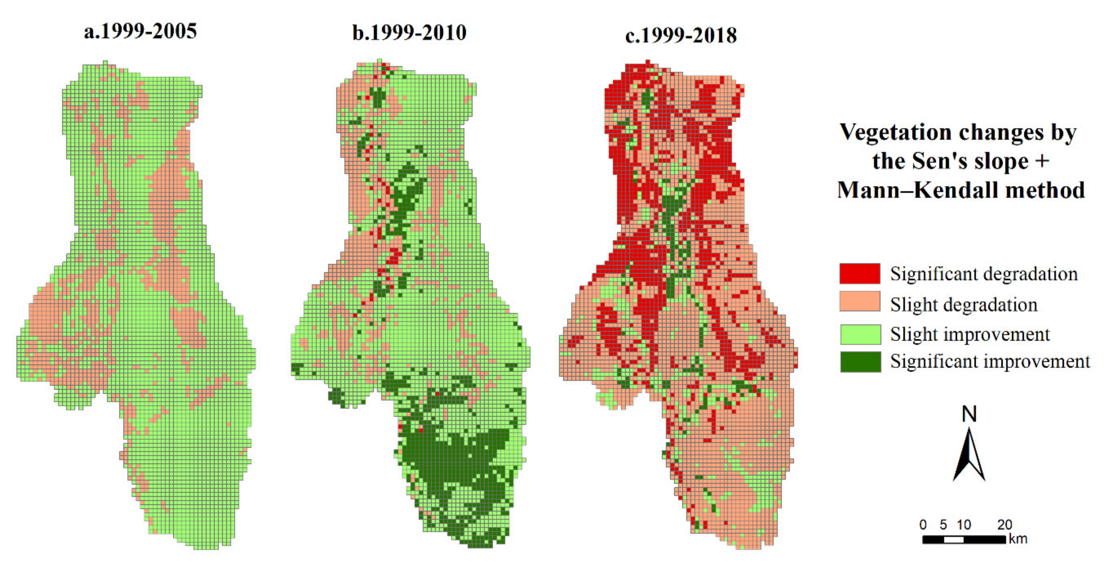
4.1. Temporal Trends and Spatial Distribution in NDVI

The tendency of vegetation changes to first rise and then quickly decline appeared in the whole study area. The proportion of the significant degradation area increased (Figure 3) according to vegetation trend analysis of Sen’s slope. Clear improvements of vegetation changes accounted for the majority of the study area (74%) in the initial stages, especially a significant improvement gathering in the south of the study area (17%) with the NDVI value increasing nearly by 100% (Figure 3b). Initially degraded areas were mainly distributed in the mining areas and eastern mountainous areas, and 85% of them turned degradation into improvement during 1999–2010. Positive growth conditions drove an upward vegetation trend in 1999–2010. Nevertheless, in 1999–2018, the overall trend of vegetation had deteriorated, and degraded areas accounted for more than 80% of the total study area (Figure 3c). Severely degraded vegetation areas (27%) were distributed in the north of the study area and mining areas. Most significant improvements in the south of the study area were lost, and continuous degradation occurred in the western areas. The few improvements that were gathered in the central town may result from ecological construction.

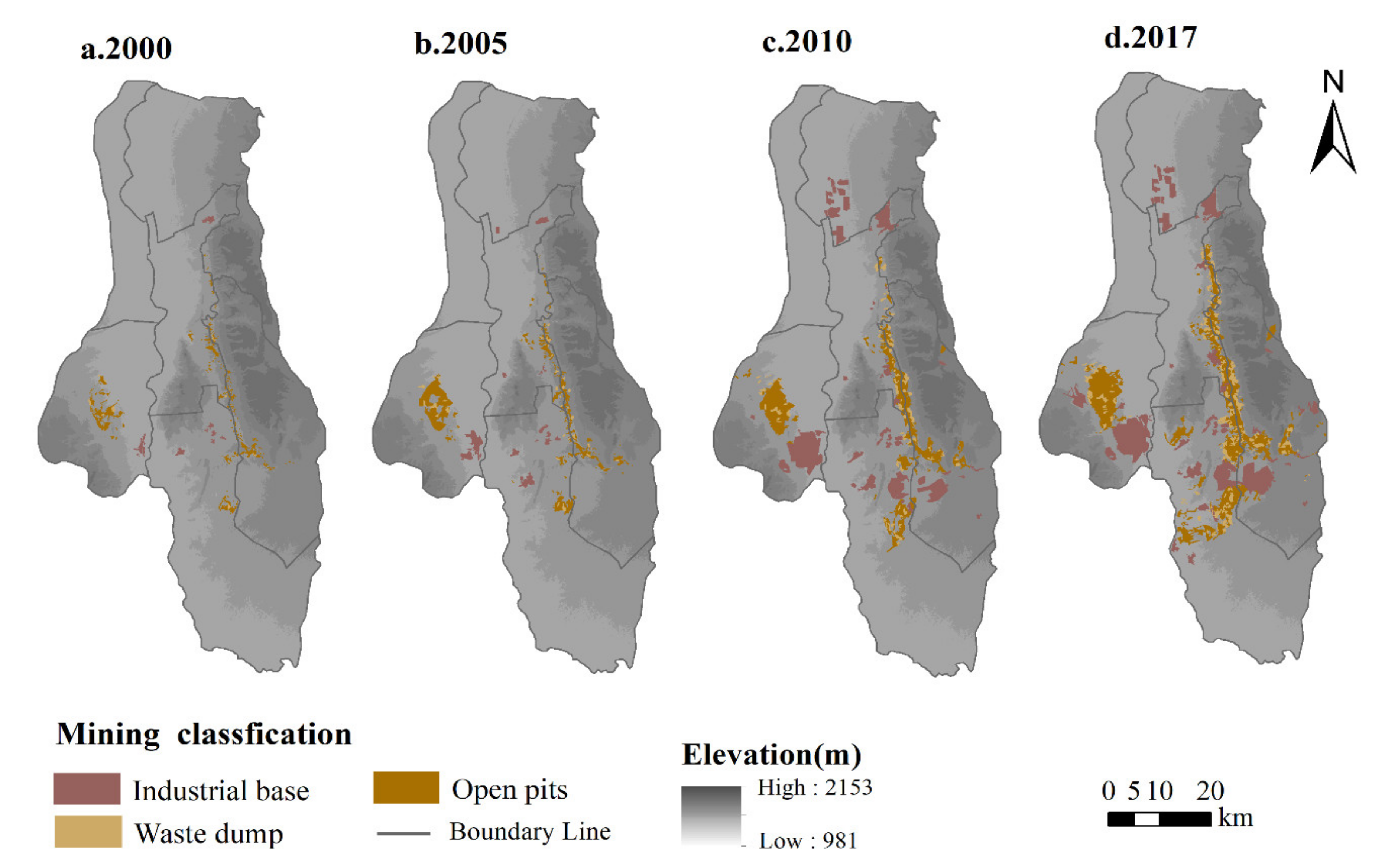
4.2. Spatiotemporal Distribution of Mining Development

Mining development rapidly expanded over the past 20 years, and established a connected spatial pattern in three major industrial bases. As shown in Figure 4, the total area of the industrial base was 9.57 km² in 2000 and 184.98 km² in 2017. Open pits gradually expanded with a uniform growth rate of 9.17 km²/a around the core industrial base, the distribution of which was in a narrow pattern along the terrain of the valley in the middle, and an aggregate pattern in the northwest of the study area. The waste dump was staggered with open pits and expanded from 2.85 km² in 2000 to 69.36 km² in 2017. Areas of mining activities expanded from 55.83 km² in 2000 to 453.78 km² in 2017, accounting for more than one-tenth of the research area and 9 times the production scale in 2000. The average expansion rate was 16%, 32%, and 7% per year in 2000–2005, 2005–2010 and 2010–2017, respectively, with the highest expansion in the period of 2005–2010, as the market price of coal was at historic highs.

4.3. Mining Development and Elevation of Influencing Vegetation Changes

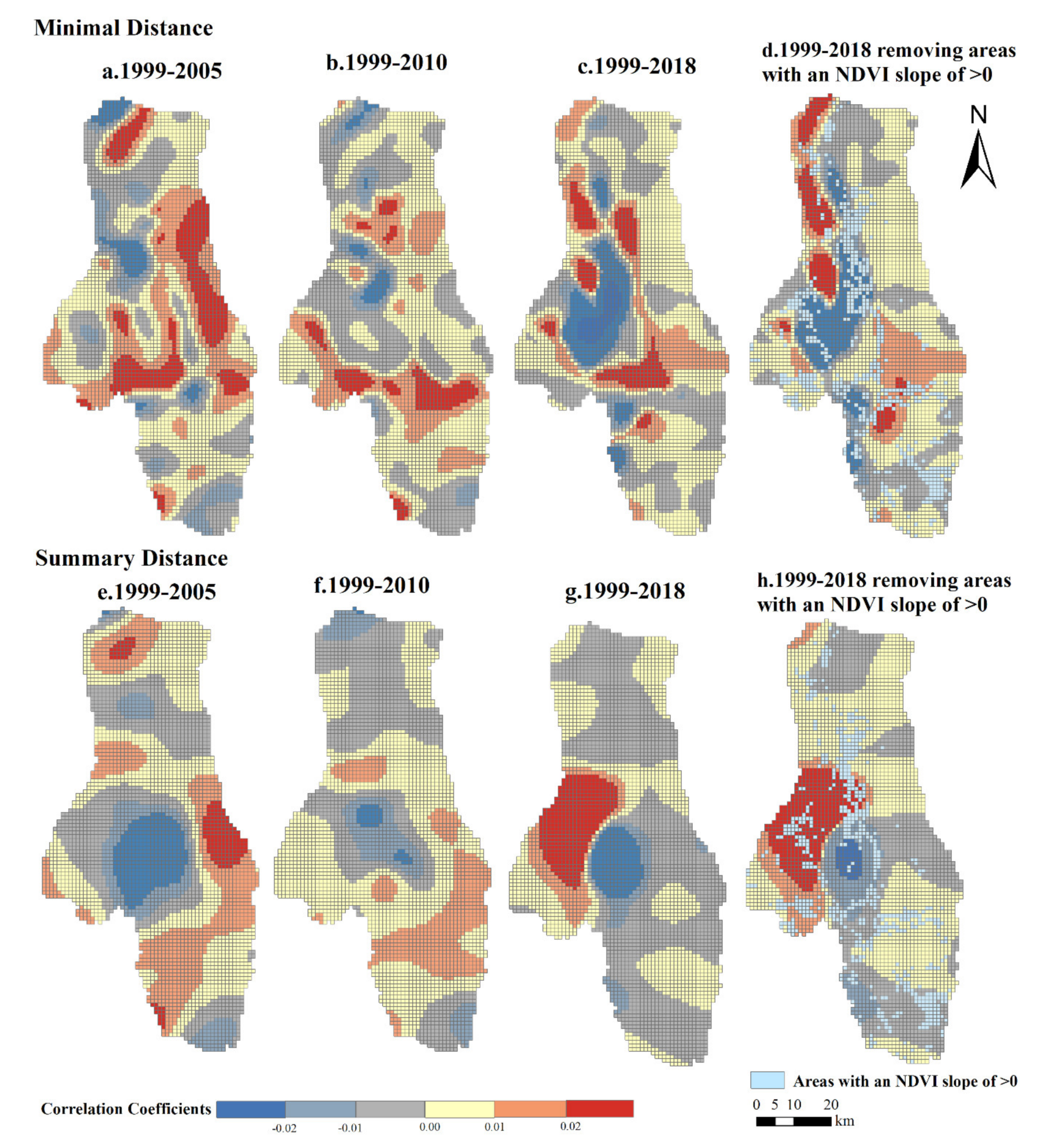
4.3.1. Correlation between Minimal Distance, Summary Distance, and Vegetation Changes

Spatial variation, mapping the relationship between distances and vegetation changes, was clearly shown in Figure 5. The positive coefficient indicated that vegetation changes moved towards an upward trend as the increase in distance to mining areas in the minimal and summary distance models. The depth of colors expressed the level of the correlation coefficient and fitness to match the variables.

For minimal distance, as distance increased, the impact of single mines on vegetation was shrunken, but dominated around areas of mining activities. Areas with positive coefficient (above 0.01) was 1418, 969, 866, and 733 km², respectively, with a continuous decline trend of 48.31%. The mean coefficient (above 0.02) continued growing by 20% (0.025, 0.026, 0.03, 0.033, respectively). Positive coefficients were significantly higher around mining areas than those of other areas, and a clear shift from negative to positive correction constantly occurred in the mining areas (Figure 5a–c). The spatial pattern of areas with higher positive correlation (above 0.01) was consistent with spatial pattern of mining development, especially in the middle of study area after removing the areas with an NDVI slope of >0.

For summary distance, in the agglomeration process of mining development, the impact of multiple mines gradually shifted from the outside to the inside and continued to be increasingly concentrated in overlapping areas of mining activities. Areas with positive correlation (above 0.01) were 1129, 704, 587, and 588 km² respectively, showing a downward trend. The higher ones (above 0.02) maintained a downward trend in the east but an increasing trend in the west, with an area of 186, 0, 393, and 373 km². The average coefficient continuously increased by 92% from 0.026 to 0.050. The increase in both the area and coefficient of positive correlation had emerged and gathered in the west overlapping areas of three industrial bases. This was more evident in the increase in areas with positive correlation after removing areas with an NDVI slope of >0, with mean coefficients of up to 0.056. The comprehensive impact of coal bases is more influential for regional vegetation changes.

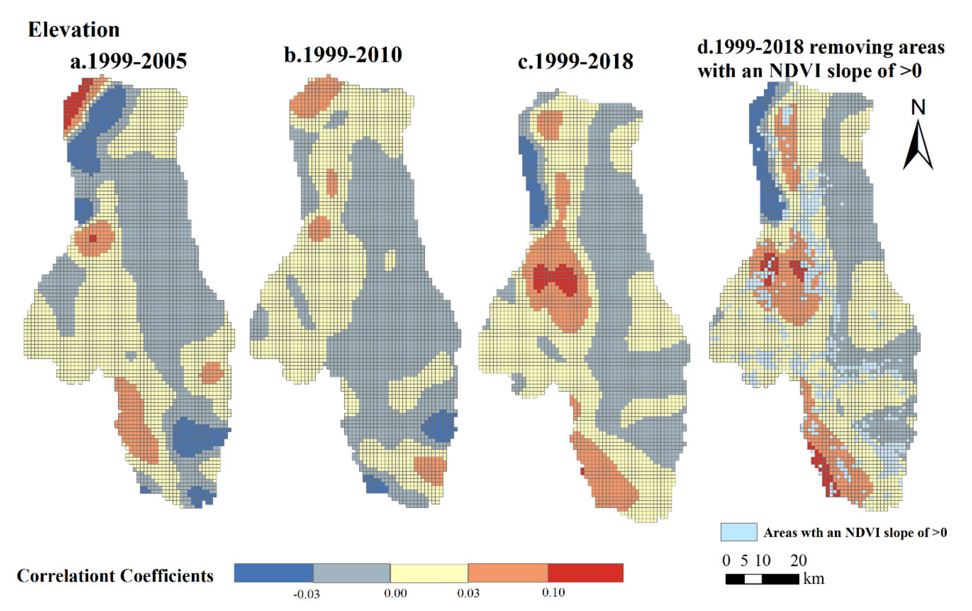
4.3.2. Correlation between Elevation and Vegetation Changes

Significant spatial differences were shown in the relationship between vegetation changes and elevation (Figure 6). The positive coefficient indicated that vegetation degradation improved with the increase in elevations, and the negative coefficient meant that vegetation degradation was worsening with the elevation’s increasing.

Spatial relationship between elevation and vegetation changes varied according to the average elevation of the total mining areas. Negative correlation in higher-elevation areas and positive correlation in low-altitude areas were expressed in the relationship between elevation and vegetation changes. The two were approximately bounded by the average elevation of the total mining areas. Most areas with negative correlation were distributed in the middle and southwest of the study area, with the proportion gradually decreasing from 56%, 62%, 47%, to 38%. Low-elevation areas in the south gradually changed from negative into positive correlation as mining activities continuously expanded, indicating that the degradation of low-elevation vegetation was more serious with the decrease in elevation. Furthermore, this may partly explain the disappearance of extremely significant improvement areas in southern areas as the Hainan industrial base agglomerating. Three positively correlated aggregation areas of about 362 km² were located in the middle, north, and south around the Yellow river and constructed areas. The boundary between positive and negative correlations (–0.03 to 0 and 0 to 0.03) was consistent with the 1200–1230 m contour line, shown in Figure 6c,d.

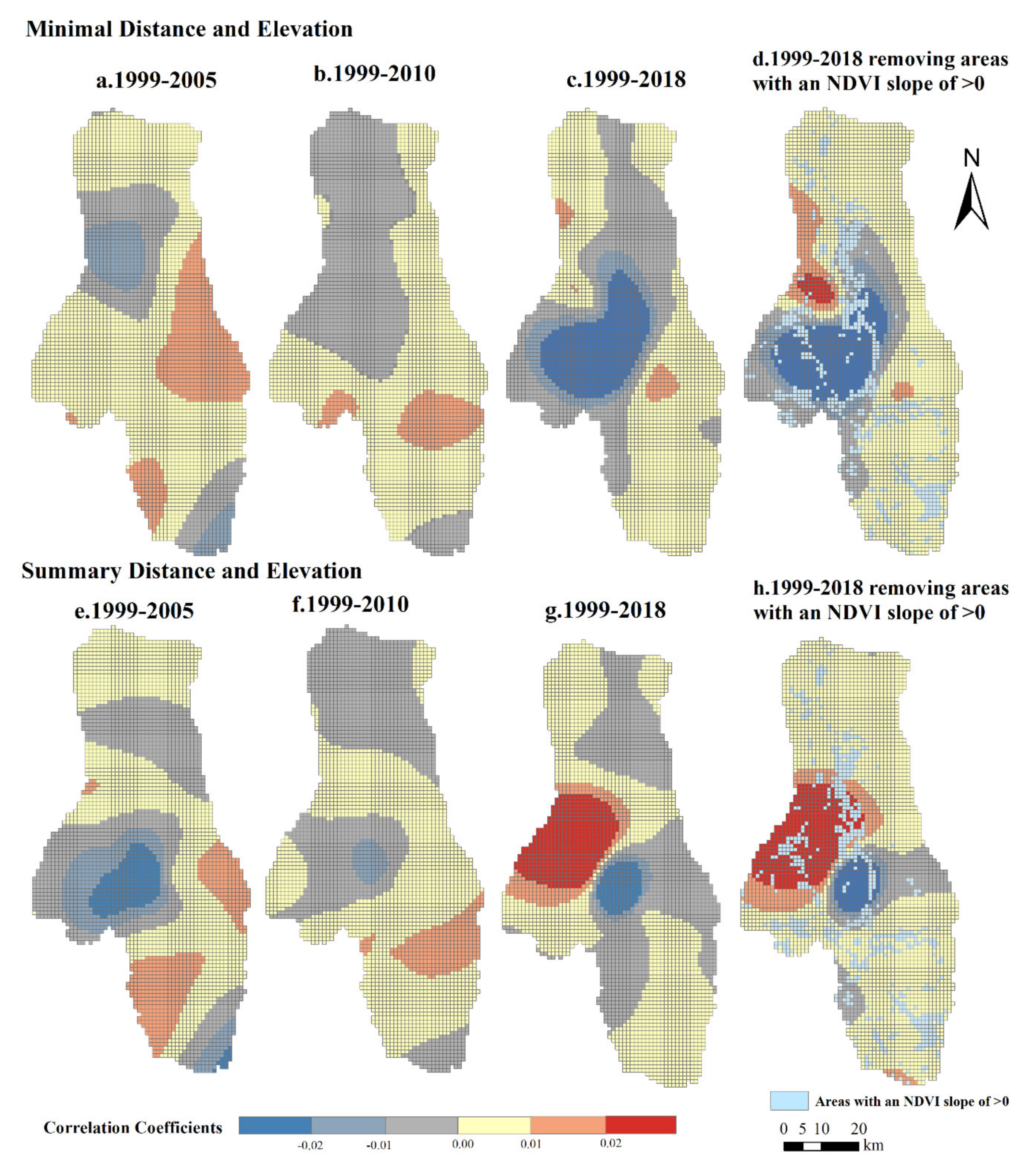
4.3.3. Correlation between Minimal Distance, Summary Distance, Elevation, and Vegetation Changes

Proper spatial stationarity was enormously maintained in maps of distance factors and vegetation changes after the combination of elevation and distances (Figure 7).

For minimal distance, quantity disappearance in positively correlated areas and expansion of negatively correlated areas, especially in the western areas, were clearly shown in the combination of minimal distance and elevation (Figure 7a–d). Such disappearance illustrated that the ecological impact of a single mine on vegetation and its action pathway were not closely related to elevation. As minimal distance to mining areas increased, elevation and distance had disproportionately opposite effects on vegetation changes at different elevation levels, as per Section 4.3.1 and Section 4.3.2.

For summary distance, the spatial distribution of positively correlated areas was relatively stable and showed no significant difference in whether elevation was involved in the relationship of summary distance and vegetation changes. Areas of positive coefficients continued growing with a proportion of up to 86.36%, and the quantities of higher positive coefficients (above 0.02) in 1999–2018 had increased by 17% compared with Figure 5e–h. Consequently, the comprehensive impact of summary distance on vegetation changes was relatively stable and not determined by the elevation, but by the spatial pattern of mining development. Moreover, after removing areas with an NDVI slope of >0, significant improvements of the positive coefficients occupied the majority, and less than 14% of the negative areas were distributed in the middle of the study area. The comprehensive ecological influence of summary distance was constantly strengthened with the systemization of mining activities.

5. Discussion

5.1. Importance of Applying GWR in Studying Spatial Heterogeneity of Vegetation

Significant spatial heterogeneity of the relationship between mining development and vegetation changes was revealed by comparing the GWR and OLS models (

Table 2. Comparison in adjusted R² of geographically weighted regression (GWR) and ordinary least squares (OLS) models.

	Adjusted R2	1999–2005	1999–2010	1999–2018	1999–2018R
Elevation	Adjusted R2G	0.27	0.31	0.50	0.59
	Adjusted R2O	0.01	0.00	0.02	0.04
Minimal distance	Adjusted R2G	0.28	0.33	0.52	0.62
	Adjusted R2O	0.05	0.04	0.00	0.00
Summary distance	Adjusted R2G	0.20	0.28	0.27	0.41
	Adjusted R2O	0.01	0.01	0.00	0.01
Minimal distance and elevation	Adjusted R2G	0.20	0.27	0.29	0.41
	Adjusted R2O	0.05	0.03	0.02	0.05
Summary distance and elevation	Adjusted R2G	0.19	0.26	0.26	0.38
	Adjusted R2O	0.02	0.01	0.02	0.06

Adjusted R²_G: adjusted R² of GWR; adjusted R²_O: adjusted R² of OLS; 1999–2018R: 1999–2018 after removing areas with normalized difference vegetation index (NDVI) slope of > 0.

and

Table 3. Comparison of Akaike information criterion (AIC) from GWR and OLS models.

	AIC	1999–2005	1999–2010	1999–2018	1999–2018R
Elevation	AICG	−31717.3	−34396.9	−32869.7	−28356.0
	AICO	−30523.8	−32951.2	−30187.1	−25504.8
Minimal distance	AICG	−31739.0	−34488.6	−33030.7	−28700.3
	AICO	−30686.0	−33086.7	−30113.6	−25358.1
Summary distance	AICG	−31367.3	−34238.5	−31372.5	−27137.2
	AICO	−30517.9	−32968.3	−30118.3	−25381.6
Minimal distance and elevation	AICG	−31364.3	−34189.6	−31489.8	−27145.2
	AICO	−30692.2	−33084.9	−30186.6	−25519.6
Summary distance and elevation	AICG	−31311.1	−34138.6	−31329.3	−26979.4
	AICO	−30549.2	−32969.9	−30214.0	−25589.5

). The adjusted R² of the GWR model was in the range of 0.19 to 0.62, which was higher and better than that of the OLS model (all less than 0.1). This showed that the GWR model could greatly explain the impact of mining on vegetation changes. Therefore, it was concluded that the spatial relationship between mining development and vegetation changes was almost not linear, but showed great spatial heterogeneity. All R² of GWR also gradually increased with the expansion and aggregation of mining development, indicating that mining development had increasingly significant impact on vegetation changes.

However, the question was why vegetation changes in the resource regions showed significant spatial heterogeneity. Numerous studies suggested that vegetation greening rate was elevation-dependent by the different sensitivity levels to precipitation and temperature changes in arid and semiarid regions [64,65,66]. In mining areas, Liu et al. [67] found significant positive correlation in the relationship between NDVI and elevation factor, while Li et al. [68] discovered that as the elevation increased, the area covered by medium and high vegetation gradually decreased. We concluded that the vegetation changes were closely related with the average elevation of mining activities, and the higher degradation rate occurred away from the average elevation of mining activities due to the gravity convergence of the basin in low elevation, and fragile conditions of vegetation growth and high external sensitivity in high elevation.

Extensive human activities, including ecological management, are other drivers to determine vegetation changes. Areas with negative correlation, where vegetation improved with the decline of summary distance to mining areas (Figure 7h), are mainly distributed in the natural protected areas with strong ecological management, though these are at the shortest distance in the summary distance model, and should be the region with the highest degradation according to the assumption. The effect of ecological protection could also be seen in the relationship between vegetation changes and elevation (Figure 6d), such as the eastern, southeastern, and northeastern areas of positive correlation. The significant improvement areas of vegetation were mainly distributed around the central town because of ecological-engineering activities. Ecological activities are important measures to maintain and improve vegetation growth, and become important factors to increase the spatial heterogeneity of vegetation changes. Furthermore, all-natural protection areas were disproportionately degraded, so existing protected areas must be strengthened, and the cumulative regionwide effects of mining activities must be mitigated [69,70,71].

5.2. Effect of Distance on Vegetation Disturbance in Mining Areas

The results suggested that the ecological impact of a single mine was continuously strengthened around the mining areas. A nationwide survey in China concluded that the distance of environmental impact from mining sites varied from a few hundred meters to 10 km [72]. Previous studies have shown that the influencing range of ecological disturbance in a single mine was mostly between 1000 and 3200 m [73,74]. In areas with poor vegetation growth conditions, the range of mining disturbance is much greater [74]. The average distance of vegetation disturbance in large mining sites is greater than that of small ones [75]. Empirical evidence from the Mongolian Plateau shows that this disturbance range of large coal exacting areas had increased to over 5 km [75], where the ecosystem could maintain stable, sustainable, and rich ecosystem services [76]. The aggregated development of mining activities enhances the range of ecological disturbance of individual mines.

For the comprehensive impact of mining activities, it is difficult to judge the distance threshold of mining disturbance. Our research results showed that its impact on vegetation changes was determined by the comprehensive spatial pattern of current and future mining development. Related scholars made some preliminary explorations. Cheng et al. [77] suggested that, in large coal bases, the source and distribution of heavy-metal pollution have significant spatial heterogeneity, there is a hot spot in the overlapping area of multiple coal mines, and the dispersion of pollutants is higher than that of single mines. Moreover, the distance of its heavy-metal pollution far exceeds the capacity of a single mine, reaching more than 15 km. In the aggregation process of mining development, the centralization effect of mining activities emerged, and was continuously enhanced and stabilized.

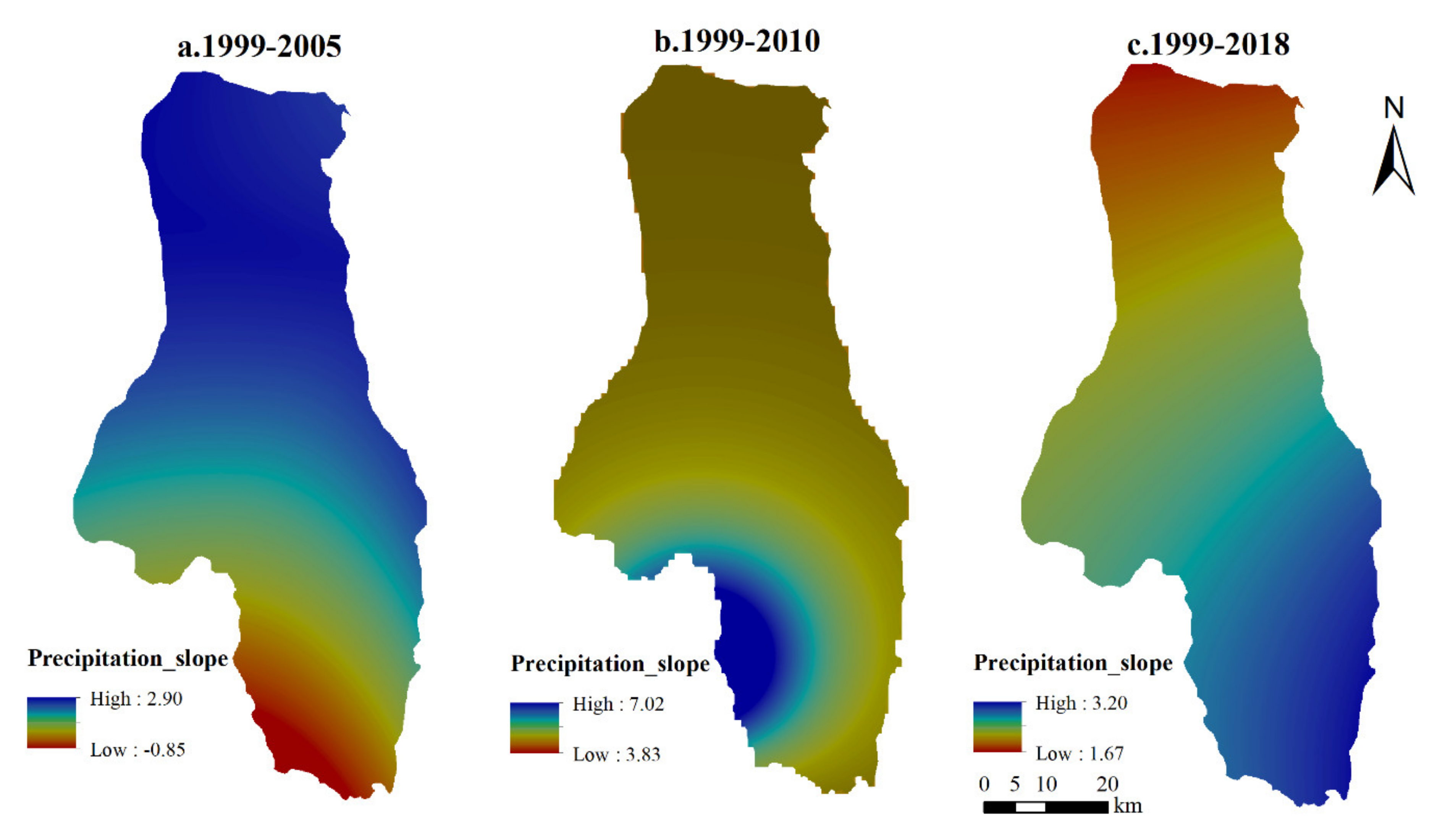
5.3. Response of Vegetation Changes to Climate Conditions

A warming–wetting trend occurred in the study area that provided excellent conditions for vegetation growth, and the increase in precipitation showed spatial differences during the last two decades (Figure 8). In the study area, the precipitation in the north was much lower than that in the south, in which the precipitation growth reached the peak of about 7 mm/a on average during 1999–2010. This strongly explained overall improvements of vegetation in the study area, especially in the south, where almost all significant improvements had emerged in 1999–2010. However, the degree of vegetation degradation was relatively high in 1999-2018, although there was a significant vegetation improvement in the previous period and a constant precipitation increase throughout the period. This properly meant that the impact that resulted from mining development was far greater than the impact of positive climate factors on vegetation during 2010–2018.

Under the context of global warming, the research area experienced notable climate change. Prior to 2010, temperature changes were relatively stable and even slightly decreased, and the average temperature then rose rapidly by about 1.5°C. Increased temperature promotes the germination of vegetation in spring and improves the growth of vegetation; on the other hand, it increases the transpiration and evaporation of plants in summer, which limits vegetation growth in arid and semiarid regions. Ma et al. [78] reported that evapotranspiration variation was consistent with changes in vegetation coverage, with a marginally increasing trend of about 0–5 mm/a during 2000–2010 and no significant increasing trend during 2011–2015 in the northwestern Loess Plateau. Numerous studies also showed that climate warming is one of the main driving factors of greening in northern China by enhancing photosynthesis and increasing vegetation activity [66,79,80,81].

In summary, climatic conditions were very favorable for the growth of vegetation during 1999–2018. It is almost impossible that climate changes led to vegetation degradation in such a water-scarce area with huge evapotranspiration, instead promoting vegetation growth.

5.4. Limitations

Although reliable and extensive data were used in this research, there were inevitable uncertainties or limitations. The interannual series of the maximal NDVI can characterize the dynamic changes of regional vegetation, but the shortage of data in some years and the image time deviation of the growing season had a specific effect on the accurate assessment of vegetation changes. More accurate time-series data and error analysis of calculation should be implemented in future studies. In addition, studies on the spatial differences of dominant areas by single mine and regional mining impacts, and their dominant areas conversion in resource regions should be strengthened in future research. Vegetation changes in resource regions are a comprehensive manifestation of indicators, such as vegetation types, climate conditions, groundwater depth, mining activities, and ecological management [30]. In relation to effect analysis of factors on vegetation, there may have been uncertainties brought about by other indicators. The contribution of other indicators to vegetation changes is notable and should be strengthened in future research.

6. Conclusions

Spatial heterogeneity is a great challenge in exploring the correlation between vegetation changes and mining development. Through spatial correlation based on the GWR model, three dominating factors were detected to quantify the correlation between vegetation changes and mining development across time and space. Our analysis indicated that incremental and combined mining activities could reverse the incremental trend of regional vegetation, leading to 86% degradation in the entire study area. Vegetation experienced a trend first of growth and then decline in the aggregation process of mining development. The scope of influence for single mines on vegetation had shrunk by about 48%, and the mean coefficients increased by 20%, closer to mining areas. The scope of influence for multiple mines on vegetation gradually expanded to 86% from the outer edge to the inner overlapping areas of mining areas, where the mean coefficients increased by 92%. Elevation dependence of vegetation changes varied according to the average elevation of total mining areas and played an important role in causing the spatial heterogeneity of mining impact on vegetation. Ecological measures should be implemented according to local conditions to achieve sustainable vegetation ecology.

References

1. Vereecken, H.; Kollet, S.; Simmer, C. Patterns in Soil-Vegetation-Atmosphere Systems: Monitoring, Modeling, and Data Assimilation. Vadose Zone J. 2010, 9, 821–827. [Google Scholar] [CrossRef]
2. Boyd, I.L.; Freer-Smith, P.H.; Gilligan, C.A.; Godfray, H.C.J. The Consequence of Tree Pests and Diseases for Ecosystem Services. Science 2013, 342, 823. [Google Scholar] [CrossRef] [PubMed]
3. Franklin, J.; Serra-Diaz, J.M.; Syphard, A.D.; Regan, H.M. Global change and terrestrial plant community dynamics. Proc. Natl. Acad. Sci. USA 2016, 113, 3725–3734. [Google Scholar] [CrossRef] [PubMed] [Green Version]
4. Fensholt, R.; Langanke, T.; Rasmussen, K.; Reenberg, A.; Prince, S.D.; Tucker, C.; Scholes, R.J.; Le, Q.B.; Bondeau, A.; Eastman, R.; et al. Greenness in semi-arid areas across the globe 1981–2007—An Earth Observing Satellite based analysis of trends and drivers. Remote Sens. Environ. 2012, 121, 144–158. [Google Scholar] [CrossRef]
5. Zhu, Z.C.; Piao, S.L.; Myneni, R.B.; Huang, M.T.; Zeng, Z.Z.; Canadell, J.G.; Ciais, P.; Sitch, S.; Friedlingstein, P.; Arneth, A.; et al. Greening of the Earth and its drivers. Nat. Clim. Chang. 2016, 6, 791–795. [Google Scholar] [CrossRef]
6. Li, F.; Wang, R.S.; Hu, D.; Ye, Y.P.; Yang, W.R.; Liu, H.X. Measurement methods and applications for beneficial and detrimental effects of ecological services. Ecol. Indic. 2014, 47, 102–111. [Google Scholar] [CrossRef]
7. United Nations(UN). Sustainable Development Goals: 17 Goals to Transform Our World. Available online: http://www.un.org/sustainabledevelopment/sustainable-development-goals/ (accessed on 3 September 2020).
8. United Nations(UN). Decade on Ecosystem Restoration 2021–2030. Available online: https://www.decadeonrestoration.org/ (accessed on 3 September 2020).
9. Hendryx, M.; Zullig, K.J.; Luo, J.H. Impacts of Coal Use on Health. In Annual Review of Public Health; Fielding, J.E., Ed.; Annual Reviews: Palo Alto, CA, USA, 2020; Volume 41, pp. 397–415. [Google Scholar]
10. Qureshi, A.A.; Kazi, T.G.; Baig, J.A.; Arain, M.B.; Afridi, H.I. Exposure of heavy metals in coal gangue soil, in and outside the mining area using BCR conventional and vortex assisted and single step extraction methods. Impact on orchard grass. Chemosphere 2020, 255, 11. [Google Scholar] [CrossRef]
11. Liu, S.L.; Li, W.P. Zoning and management of phreatic water resource conservation impacted by underground coal mining: A case study in arid and semiarid areas. J. Clean. Prod. 2019, 224, 677–685. [Google Scholar] [CrossRef]
12. Ma, K.; Zhang, Y.X.; Ruan, M.Y.; Guo, J.; Chai, T.Y. Land Subsidence in a Coal Mining Area Reduced Soil Fertility and Led to Soil Degradation in Arid and Semi-Arid Regions. Int. J. Environ. Res. Public Health 2019, 16, 3929. [Google Scholar] [CrossRef] [Green Version]
13. Martins, W.B.R.; Lima, M.D.R.; Barros, U.D.; Amorim, L.; Oliveira, F.D.; Schwartz, G. Ecological methods and indicators for recovering and monitoring ecosystems after mining: A global literature review. Ecol. Eng. 2020, 145, 11. [Google Scholar] [CrossRef]
14. Xu, J.P.; Ma, N.; Xie, H.P. Ecological coal mining based dynamic equilibrium strategy to reduce pollution emissions and energy consumption. J. Clean. Prod. 2017, 167, 514–529. [Google Scholar] [CrossRef]
15. Kompala-Baba, A.; Bierza, W.; Blonska, A.; Sierka, E.; Magurno, F.; Chmura, D.; Besenyei, L.; Radosz, L.; Wozniak, G. Vegetation diversity on coal mine spoil heaps—How important is the texture of the soil substrate? Biologia 2019, 74, 419–436. [Google Scholar] [CrossRef] [Green Version]
16. Lefticariu, L.; Walters, E.R.; Pugh, C.W.; Bender, K.S. Sulfate reducing bioreactor dependence on organic substrates for remediation of coal-generated acid mine drainage: Field experiments. Appl. Geochem. 2015, 63, 70–82. [Google Scholar] [CrossRef]
17. Fiket, Z.; Medunic, G.; Vidakovic-Cifrek, Z.; Jezidzic, P.; Cvjetko, P. Effect of coal mining activities and related industry on composition, cytotoxicity and genotoxicity of surrounding soils. Environ. Sci. Pollut. Res. 2020, 27, 6613–6627. [Google Scholar] [CrossRef] [PubMed]
18. Artico, L.L.; Kommling, G.; Migita, N.A.; Menezes, A.P.S. Toxicological Effects of Surface Water Exposed to Coal Contamination on the Test System Allium cepa. Water Air Soil Pollut. 2018, 229, 12. [Google Scholar] [CrossRef]
19. Freitas, L.A.d.; Rambo, C.L.; Franscescon, F.; Barros, A.F.P.d.; Lucca, G.d.S.D.; Siebel, A.M.; Scapinello, J.; Lucas, E.M.; Magro, J.D. Coal extraction causes sediment toxicity in aquatic environments in Santa Catarina, Brazil. Rev. Ambiente Água 2017, 12, 591–604. [Google Scholar] [CrossRef] [Green Version]
20. Wang, Z.Y.; Hou, J.; Guo, J.Y.; Wang, C.J.; Wang, M.J. Coal Dust Reduce the Rate of Root Growth and Photosynthesis of Five Plant Species in Inner Mongolian Grassland. J. Residuals Sci. Technol. 2016, 13, S63–S73. [Google Scholar]
21. Shi, Y.K.; Mu, X.M.; Li, K.R.; Shao, H.B. Soil characterization and differential patterns of heavy metal accumulation in woody plants grown in coal gangue wastelands in Shaanxi, China. Environ. Sci. Pollut. Res. 2016, 23, 13489–13497. [Google Scholar] [CrossRef]
22. Sun, L.; Liao, X.Y.; Yan, X.L.; Zhu, G.H.; Ma, D. Evaluation of heavy metal and polycyclic aromatic hydrocarbons accumulation in plants from typical industrial sites: Potential candidate in phytoremediation for co-contamination. Environ. Sci. Pollut. Res. 2014, 21, 12494–12504. [Google Scholar] [CrossRef]
23. National Development and Reform Commission; PRC. 13th Five-Year Plan for Coal Industry Development. Available online: https://www.ndrc.gov.cn/xxgk/zcfb/ghwb/201612/t20161230_962216.html (accessed on 19 September 2020).
24. Giam, X.; Olden, J.D.; Simberloff, D. Impact of coal mining on stream biodiversity in the US and its regulatory implications. Nat. Sustain. 2018, 1, 176–183. [Google Scholar] [CrossRef]
25. Zeng, Q.; Shen, L.; Yang, J. Potential impacts of mining of super-thick coal seam on the local environment in arid Eastern Junggar coalfield, Xinjiang region, China. Environ. Earth Sci. 2020, 79, 15. [Google Scholar] [CrossRef]
26. Li, Y.M.; Zhang, B.; Wang, B.; Wang, Z.H. Evolutionary trend of the coal industry chain in China: Evidence from the analysis of I-O and APL model. Resour. Conserv. Recycl. 2019, 145, 399–410. [Google Scholar] [CrossRef]
27. Zhang, Y.Q.; Wu, D.; Wang, C.X.; Fu, X.; Wu, G. Impact of coal power generation on the characteristics and risk of heavy metal pollution in nearby soil. Ecosyst. Health Sustain. 2020, 6, 12. [Google Scholar] [CrossRef]
28. Franks, D.M.; Brereton, D.; Moran, C.J. The cumulative dimensions of impact in resource regions. Resour. Policy 2013, 38, 640–647. [Google Scholar] [CrossRef]
29. Porter, M.; Franks, D.M.; Everingham, J.A. Cultivating collaboration: Lessons from initiatives to understand and manage cumulative impacts in Australian resource regions. Resour. Policy 2013, 38, 657–669. [Google Scholar] [CrossRef]
30. Liu, S.L.; Li, W.P.; Qiao, W.; Wang, Q.Q.; Hu, Y.B.; Wang, Z.K. Effect of natural conditions and mining activities on vegetation variations in arid and semiarid mining regions. Ecol. Indic. 2019, 103, 331–345. [Google Scholar] [CrossRef]
31. Pei, H.; Fang, S.F.; Lin, L.; Qin, Z.H.; Wang, X.Y. Methods and applications for ecological vulnerability evaluation in a hyper-arid oasis: A case study of the Turpan Oasis, China. Environ. Earth Sci. 2015, 74, 1449–1461. [Google Scholar] [CrossRef] [Green Version]
32. Fang, A.M.; Dong, J.H.; Cao, Z.G.; Zhang, F.; Li, Y.F. Tempo-Spatial Variation of Vegetation Coverage and Influencing Factors of Large-Scale Mining Areas in Eastern Inner Mongolia, China. Int. J. Environ. Res. Public Health 2020, 17, 47. [Google Scholar] [CrossRef] [Green Version]
33. Li, Y.R.; Cao, Z.; Long, H.L.; Liu, Y.S.; Li, W.J. Dynamic analysis of ecological environment combined with land cover and NDVI changes and implications for sustainable urban-rural development: The case of Mu Us Sandy Land, China. J. Clean. Prod. 2017, 142, 697–715. [Google Scholar] [CrossRef]
34. McMillen, D.P. Geographically Weighted Regression: The Analysis of Spatially Varying Relationships. Am. J. Agric. Econ. 2004, 86, 554–556. [Google Scholar] [CrossRef]
35. Li, H.L.; Peng, J.; Liu, Y.X.; Hu, Y.N. Urbanization impact on landscape patterns in Beijing City, China: A spatial heterogeneity perspective. Ecol. Indic. 2017, 82, 50–60. [Google Scholar] [CrossRef]
36. Tenerelli, P.; Demsar, U.; Luque, S. Crowdsourcing indicators for cultural ecosystem services: A geographically weighted approach for mountain landscapes. Ecol. Indic. 2016, 64, 237–248. [Google Scholar] [CrossRef] [Green Version]
37. Dadashpoor, H.; Azizi, P.; Moghadasi, M. Land use change, urbanization, and change in landscape pattern in a metropolitan area. Sci. Total Environ. 2019, 655, 707–719. [Google Scholar] [CrossRef] [PubMed]
38. Shaker, R.R.; Altman, Y.; Deng, C.B.; Vaz, E.; Forsythe, K.W. Investigating urban heat island through spatial analysis of New York City streetscapes. J. Clean. Prod. 2019, 233, 972–992. [Google Scholar] [CrossRef]
39. Liu, Y.; Zhao, N.Z.; Vanos, J.K.; Cao, G.F. Revisiting the estimations of PM2.5-attributable mortality with advancements in PM2.5 mapping and mortality statistics. Sci. Total Environ. 2019, 666, 499–507. [Google Scholar] [CrossRef]
40. Xia, C.; Xiang, M.; Fang, K.; Li, Y.; Ye, Y.; Shi, Z.; Liu, J. Spatial-temporal distribution of carbon emissions by daily travel and its response to urban form: A case study of Hangzhou, China. J. Clean. Prod. 2020, 257, 120797. [Google Scholar] [CrossRef]
41. Sannigrahi, S.; Zhang, Q.; Pilla, F.; Joshi, P.K.; Basu, B.; Keesstra, S.; Roy, P.S.; Wang, Y.; Sutton, P.C.; Chakraborti, S.; et al. Responses of ecosystem services to natural and anthropogenic forcings: A spatial regression based assessment in the world’s largest mangrove ecosystem. Sci. Total Environ. 2020, 715, 13. [Google Scholar] [CrossRef]
42. Sun, X.; Tang, H.J.; Yang, P.; Hu, G.; Liu, Z.H.; Wu, J.G. Spatiotemporal patterns and drivers of ecosystem service supply and demand across the conterminous United States: A multiscale analysis. Sci. Total Environ. 2020, 703, 17. [Google Scholar] [CrossRef] [PubMed]
43. Sawut, R.; Kasim, N.; Abliz, A.; Li, H.; Yalkun, A.; Maihemuti, B.; Shi, Q.D. Possibility of optimized indices for the assessment of heavy metal contents in soil around an open pit coal mine area. Int. J. Appl. Earth Obs. Geoinf. 2018, 73, 14–25. [Google Scholar] [CrossRef]
44. Intergovernmental Panel on Climate Change(IPCC). Special Report On Climate Change And Land: Desertification. Available online: https://www.ipcc.ch/srccl/chapter/chapter-3/ (accessed on 18 September 2020).
45. Mancini, L.; Sala, S. Social impact assessment in the mining sector: Review and comparison of indicators frameworks. Resour. Policy 2018, 57, 98–111. [Google Scholar] [CrossRef]
46. International Energy Agency (IEA). World Energy Outlook 2017: China. Available online: https://www.iea.org/reports/world-energy-outlook-2017-china (accessed on 18 September 2020).
47. Bu, Q.W.; Li, Q.S.; Zhang, H.D.; Cao, H.M.; Gong, W.W.; Zhang, X.; Ling, K.; Cao, Y.B. Concentrations, Spatial Distributions, and Sources of Heavy Metals in Surface Soils of the Coal Mining City Wuhai, China. J. Chem. 2020, 2020, 10. [Google Scholar] [CrossRef]
48. Wang, W.F.; Hao, W.D.; Sian, Z.F.; Lei, S.G.; Wang, X.S.; Sang, S.X.; Xu, S.C. Effect of coal mining activities on the environment of Tetraena mongolica in Wuhai, Inner Mongolia, China-A geochemical perspective. Int. J. Coal Geol. 2014, 132, 94–102. [Google Scholar] [CrossRef]
49. Guan, Q.Y.; Wang, L.; Pan, B.T.; Guan, W.Q.; Sun, X.Z.; Cai, A. Distribution features and controls of heavy metals in surface sediments from the riverbed of the Ningxia-Inner Mongolian reaches, Yellow River, China. Chemosphere 2016, 144, 29–42. [Google Scholar] [CrossRef] [PubMed]
50. Dai, S.W.; Shulski, M.D.; Hubbard, K.G.; Takle, E.S. A spatiotemporal analysis of Midwest US temperature and precipitation trends during the growing season from 1980 to 2013. Int. J. Clim. 2016, 36, 517–525. [Google Scholar] [CrossRef] [Green Version]
51. Ministry of Ecology and Environment; PRC. List of National Nature Reserves. Available online: http://www.gov.cn/guoqing/2019-04/09/content_5380702.htm (accessed on 19 September 2020).
52. Batunacun; Wieland, R.; Lakes, T.; Hu, Y.F.; Nendel, C. Identifying drivers of land degradation in Xilingol, China, between 1975 and 2015. Land Use Policy 2019, 83, 543–559. [Google Scholar] [CrossRef]
53. Xue, J.R.; Su, B.F. Significant Remote Sensing Vegetation Indices: A Review of Developments and Applications. J. Sens. 2017, 2017, 17. [Google Scholar] [CrossRef] [Green Version]
54. Maneja, R.H.; Miller, J.D.; Li, W.Z.; El-Askary, H.; Flandez, A.V.B.; Dagoy, J.J.; Alcaria, J.F.A.; Basali, A.U.; Al-Abdulkader, K.A.; Loughland, R.A.; et al. Long-term NDVI and recent vegetation cover profiles of major offshore island nesting sites of sea turtles in Saudi waters of the northern Arabian Gulf. Ecol. Indic. 2020, 117, 13. [Google Scholar] [CrossRef]
55. Schell, J.A. Monitoring vegetation systems in the great plains with ERTS. Nasa Spec. Publ. 1973, 351, 309. [Google Scholar]
56. Gocic, M.; Trajkovic, S. Analysis of changes in meteorological variables using Mann-Kendall and Sen’s slope estimator statistical tests in Serbia. Glob. Planet. Chang. 2013, 100, 172–182. [Google Scholar] [CrossRef]
57. Sen, P.K. Estimates of the Regression Coefficient Based on Kendall’s Tau. J. Am. Stat. Assoc. 1968, 63, 1379–1389. [Google Scholar] [CrossRef]
58. Pingale, S.M.; Khare, D.; Jat, M.K.; Adamowski, J. Spatial and temporal trends of mean and extreme rainfall and temperature for the 33 urban centers of the arid and semi-arid state of Rajasthan, India. Atmos. Res. 2014, 138, 73–90. [Google Scholar] [CrossRef]
59. Mann, H.B. Nonparametric test against trend. Econometrica 1945, 13, 245–259. [Google Scholar] [CrossRef]
60. Kendall, M.G. Rank Correlation Methods; [Oxford University Press, Biometrika Trust]; Griffin: London, UK, 1957; Volume 44, p. 298. [Google Scholar]
61. Brunsdon, C.; Fotheringham, S.; Charlton, M. Geographically Weighted Regression-Modelling Spatial Non-Stationarity. J. R. Stat. Soc. Ser. D (Stat.) 1998, 47, 431–443. [Google Scholar] [CrossRef]
62. Alahmadi, S.; Al-Ahmadi, K.; Almeshari, M. Spatial variation in the association between NO2 concentrations and shipping emissions in the Red Sea. Sci. Total Environ. 2019, 676, 131–143. [Google Scholar] [CrossRef]
63. Marquardt, D.W. Generalized Inverses, Ridge Regression, Biased Linear Estimation, and Nonlinear Estimation. Technometrics 1970, 12, 591–612. [Google Scholar] [CrossRef]
64. Qi, X.Z.; Jia, J.H.; Liu, H.Y.; Lin, Z.S. Relative importance of climate change and human activities for vegetation changes on China’s silk road economic belt over multiple timescales. Catena 2019, 180, 224–237. [Google Scholar] [CrossRef]
65. Tai, X.L.; Epstein, H.E.; Li, B. Elevation and Climate Effects on Vegetation Greenness in an Arid Mountain-Basin System of Central Asia. Remote Sens. 2020, 12, 1665. [Google Scholar] [CrossRef]
66. Zhu, Y.K.; Zhang, J.T.; Zhang, Y.Q.; Qin, S.G.; Shao, Y.Y.; Gao, Y. Responses of vegetation to climatic variations in the desert region of northern China. Catena 2019, 175, 27–36. [Google Scholar] [CrossRef]
67. Liu, X.Y.; Zhou, W.; Bai, Z.K. Vegetation coverage change and stability in large open-pit coal mine dumps in China during 1990-2015. Ecol. Eng. 2016, 95, 447–451. [Google Scholar] [CrossRef]
68. Li, X.H.; Lei, S.G.; Cheng, W.; Liu, F.; Wang, W.Z. Spatio-temporal dynamics of vegetation in Jungar Banner of China during 2000–2017. J. Arid Land 2019, 11, 837–854. [Google Scholar] [CrossRef] [Green Version]
69. Duran, A.P.; Rauch, J.; Gaston, K.J. Global spatial coincidence between protected areas and metal mining activities. Biol. Conserv. 2013, 160, 272–278. [Google Scholar] [CrossRef]
70. Neri, A.C.; Dupin, P.; Sanchez, L.E. A pressure-state-response approach to cumulative impact assessment. J. Clean. Prod. 2016, 126, 288–298. [Google Scholar] [CrossRef]
71. Siqueira-Gay, J.; Sonter, L.J.; Sánchez, L.E. Exploring potential impacts of mining on forest loss and fragmentation within a biodiverse region of Brazil’s northeastern Amazon. Resour. Policy 2020, 67, 101662. [Google Scholar] [CrossRef]
72. Ministry of Natural Resources; PRC. The Report on the National General Survey of Soil Contamination. Available online: http://g.mnr.gov.cn/201701/t20170123_1428712.html (accessed on 3 September 2020).
73. Liao; Liu, F. Identifying the Mining Impact Range on the Vegetation of Yangquan Coal Mining Region by Using 3S Technology. J. Nat. Resour. 2010, 25, 185–191. [Google Scholar]
74. Yao, F.; Guli, J.; Bao, A.; Zhang, J.; Li, C.; Liu, J. Damage assessment of the vegetable types based on remote sensing in the open coalmine of arid desert area. China Environ. Sci. 2013, 33, 707–713. [Google Scholar]
75. Ma, Q.; He, C.Y.; Fang, X.N. A rapid method for quantifying landscape-scale vegetation disturbances by surface coal mining in arid and semiarid regions. Landsc. Ecol. 2018, 33, 2061–2070. [Google Scholar] [CrossRef]
76. Lv, X.J.; Xiao, W.; Zhao, Y.L.; Zhang, W.K.; Li, S.C.; Sun, H.X. Drivers of spatio-temporal ecological vulnerability in an arid, coal mining region in Western China. Ecol. Indic. 2019, 106, 18. [Google Scholar] [CrossRef]
77. Cheng, W.; Lei, S.G.; Bian, Z.F.; Zhao, Y.B.; Li, Y.C.; Gan, Y.D. Geographic distribution of heavy metals and identification of their sources in soils near large, open-pit coal mines using positive matrix factorization. J. Hazard. Mater. 2020, 387, 11. [Google Scholar] [CrossRef]
78. Ma, Z.; Yan, N.; Wu, B.; Stein, A.; Zhu, W.; Zeng, H. Variation in actual evapotranspiration following changes in climate and vegetation cover during an ecological restoration period (2000–2015) in the Loess Plateau, China. Sci Total Environ. 2019, 689, 534–545. [Google Scholar] [CrossRef]
79. Forzieri, G.; Alkama, R.; Miralles, D.G.; Cescatti, A. Response to Comment on “Satellites reveal contrasting responses of regional climate to the widespread greening of Earth”. Science 2018, 360, 3. [Google Scholar] [CrossRef] [Green Version]
80. Li, Z.Y.; Ma, W.H.; Liang, C.Z.; Liu, Z.L.; Wang, W.; Wang, L.X. Long-term vegetation dynamics driven by climatic variations in the Inner Mongolia grassland: Findings from 30-year monitoring. Landsc. Ecol. 2015, 30, 1701–1711. [Google Scholar] [CrossRef]
81. Piao, S.L.; Yin, G.D.; Tan, J.G.; Cheng, L.; Huang, M.T.; Li, Y.; Liu, R.G.; Mao, J.F.; Myneni, R.B.; Peng, S.S.; et al. Detection and attribution of vegetation greening trend in China over the last 30 years. Glob. Chang. Biol. 2015, 21, 1601–1609. [Google Scholar] [CrossRef] [PubMed]
Figure 1. (ab) Location, administrative divisions, land-use and land-cover map (a), and topography (b) of study area. Land-use and land-cover map was monitored at 2017, provided by the Institute of Geographic Sciences and Natural Resources Research in China. Note: districts of ①, Uulan Buh; ②, Mengxi; ③, Wuda; ④, Haibowan; ⑤, Etuoke Banner; and ⑥, Hainan.
Remotesensing 12 03247 g001
Figure 2. Framework of data processing flow.
Remotesensing 12 03247 g002
Figure 3. (ac) Spatial distribution of vegetation changes by Sen’s slope and Mann–Kendall method. (a) 1999–2005; (b) 1999–2010; (c)1999–2018.
Remotesensing 12 03247 g003
Figure 4. (ad) Components and spatial distribution of mining activities in study area.
Remotesensing 12 03247 g004
Figure 5. (ah) Spatial patterns of correlation coefficients between distance and vegetation changes. (ad) Minimal and (eh) summary distance in 1999–2018.
Remotesensing 12 03247 g005
Figure 6. (ad) Spatial patterns of correlation coefficients between elevation and vegetation changes in 1999–2018.
Remotesensing 12 03247 g006
Figure 7. (ah) Spatial patterns of correlation coefficients between distance and vegetation changes. (ad) Minimal distance and elevation, and (eh) summary distance and elevation in 1999–2018.
Remotesensing 12 03247 g007
Figure 8. (ac) Spatial distribution of precipitation slope by Kriging interpolation. Precipitation data in 1999–2018 were acquired from five meteorological reference stations: Hanjinqi, Linhe, Huinong, Etuokeqi, and Taole. Precipitation slope was obtained by linear regression based on interannual precipitation data, and then imported into ArcGIS to obtain changes in the study area by Kriging interpolation.
Remotesensing 12 03247 g008