Technical Note

Application of the Msplit Estimation Method in the Detection and Dimensioning of the Displacement of Adjacent Planes

by
Joanna Janicka
1,*,
Jacek Rapiński
1,
Wioleta Błaszczak-Bąk
1 and
Czesław Suchocki
2
1
Faculty of Geoengineering, University of Warmia and Mazury in Olsztyn, ul. Oczapowskiego 1, 10-719 Olsztyn, Poland
2
Faculty of Civil Engineering Environmental and Geodetic Sciences, Koszalin University of Technology, ul. Sniadeckich 2, 75-453 Koszalin, Poland
*
Author to whom correspondence should be addressed.
Remote Sens. 2020, 12(19), 3203; https://doi.org/10.3390/rs12193203
Submission received: 10 September 2020 / Accepted: 25 September 2020 / Published: 30 September 2020
(This article belongs to the Special Issue Geoinformation Technologies in Civil Engineering and the Environment)

Abstract

:
Building constructions are exposed to various forces and natural phenomena. Some of them are sudden and violent, e.g., an earthquake or heavy rains, causing a displacement of the ground. Other phenomena affect objects on a longer-term, e.g., vibrations caused by daily road traffic. Sometimes, building structures may have defects due to incorrect construction. In any case, if an engineering object shows changes in the relation to its correct geometry or position, deformation and displacement measurements are required. Engineering objects are also monitored during their construction. Nowadays, it is important to perform measurements quickly and with high accuracy. The use of a Terrestrial Laser Scanning (TLS) allows for the required measurement speed and accuracy. This measurement technology allows a large dataset, which can be arbitrarily elaborated, to be obtained. The structure of building objects can include vertices, lines, planes, and other shapes and can be described using mathematical functions. This allows data processing to be automated. In this article, we present the Msplit method as an effective approach to the processing of data obtained as a result of TLS measurements. The proposed approach is new because until now, the Msplit estimation method has not been used to detect adjacent planes in one-point cloud obtained from TLS. The Msplit estimation method allows a functional model to be split into two or more competitive models and thus two or more entities in a point cloud to be estimated simultaneously. Four different objects measured using TLS are presented: two objects representing vertical displacements and two objects representing horizontal displacements. The test results and analysis confirm that the Msplit estimation method can be successfully applied in the detection of adjacent planes.

1. Introduction

Monitoring the structure of an object is of great importance with respect to the reliability assessment, damage detection, and assessment of the object’s condition. Control measurements can be performed in different ways, depending on the type of construction, measurement range, and equipment used. Moreover, the classic approach also requires the involvement of a building inspector, who assesses the technical condition of the object, performs a series of measurements, makes drawings, takes photos, and analyzes the collected data. Usually, these measurements are performed using standard geodetic methods, such as the total station [1,2,3], digital photogrammetry [4], and Global Navigation Satellite System (GNSS) methods [5].
Nowadays, the use of terrestrial laser scanners (TLSs) is gaining more and more attention and application as a fast, accurate, and non-destructive measurement method (NDT) [6,7,8].
TLS technology is an active remote sensing technique widely used in civil engineering measurements. In recent years, laser scanning has found an application in many fields, e.g., the measurement of historic and archaeological objects [9,10,11] geotechnical measurements [12,13,14,15], and building condition diagnostics [16,17]. It is also increasingly used in civil engineering measurements. Measurements of large engineering structures, such as dams, bridge structures, and complex engineering structures, e.g., refineries, have long been the subject of measurements using TLS. It can also be used to monitor not only special facilities, but also everyday objects, e.g., streets and residential buildings, and it can be successfully used to obtain information about changes in the structure of an object.
TLS allows data to be acquired as a point cloud of a varying resolution. Each measured point has 3D coordinates (X, Y, Z), an intensity parameter, and semantic information (RGB). Thus, very detailed data about the object are obtained, which can, in the next step, be analyzed.
An important aspect of the development of a dataset obtained as a result of TLS measurements is the maximum possible automation of this process. The structure of a building can be represented as a set of geometric primitives, like vertices, lines, planes, or other shapes, which can be described by mathematical functions. This allows the processing of the data to be automated. This topic was discussed in many publications, for example, in [18,19,20]. With this assumption, it is possible to analyze, e.g., the wall planarity, edge verticality, or vertical and horizontal displacements of a building. In the case of testing the displacement of two elements that constitute two primitives (e.g., planes), the Msplit estimation method can be used. The method developed by Prof. Wisniewski [21] allows a functional model to be split into two or more models and thus two functional models to be identified from a single dataset.
So far, the Msplit estimation method has been used in various studies, for example, as a method of filtering data from airborne laser scanning [22]. The idea of Msplit estimation refers to the widely-known method for the elimination of gross errors (or outliers), called robust M-estimation. Applying this principle in ALS point cloud processing, points that do not belong to the terrain surface can be treated as outliers and eliminated from the DTM creation process. Msplit estimation was also used as a method for robust coordinate transformation [23].
The next application of the Msplit method was as an estimation method in the context of the analysis of the vertical displacement of geodetic points [24] or for detecting circular objects in a point cloud [25].
The results obtained by other researchers using the Msplit method undoubtedly show the potential of the application of the Msplit method in laser scanning data processing. Therefore, in this paper, the authors propose a new, as yet unexplored use of the Msplit method, which consists of fitting two planes to a point cloud acquired from the TLS of displaced planar objects. These objects are shifted relative to each other as a result of natural phenomena and exploitation. This approach allows for the dimensioning of the displacements of objects relative to other objects. This is a very important property from the point of view of construction engineering and building safety.

2. Materials and Methods

2.1. Msplit Estimation Theoretical Background

The proposed estimation method using the Msplit method allows two or more surfaces to be detected by splitting the functional model into two or more competitive models. The models are estimated from one-point cloud. It is not necessary to divide the cloud into individuals representing selected areas or to perform a measurement of each surface separately. Of course, there are some limitations to this method. Firstly, these surfaces must be displaced relative to other surfaces.
The Msplit estimation method assumes that every measurement result can be a realization of either of two or more different random variables. This estimation method was introduced by Wisniewski and is described in [26].

2.1.1. Msplit Estimation

Based on the assumption that the functional model is split into two competitive models Yα or Yβ, each observation has its own “split potential”, i.e., the probability of belonging to one of the random variables. Therefore, the observation set Ω = {yi: i = 1, 2, …, n} is a disordered mixture of the elements assigned to the random variables yα or yβ in an unknown way. For that reason, each observation Yi may have either of two competitive expected values Eα{Yi} = E{Yα} or Eβ{Yi} = E{Yβ}. In this paper, the functional model V = AX + L is split into two competitive ones, which concern the same vector of observation L:
s p l i t ( V = A X + L ) = { V α = A X α + L V β = A X β + L
where A is a common coefficient matrix, Vα and Vβ are competitive vectors of random variables, and Xα and Xβ are competitive parameter vectors. To achieve this task, a cross-weighting procedure must be introduced. The estimation of the competitive vectors (Xα and Xβ) of the parameters using the same observation vector L requires a specially formulated objective function. The proposed method replaces function ρ(v) with functions ρα (vα) and ρβ (vβ), according to the Equation (2) and in compliance with the cross-weighting Vα and Vβ. The weights of the observations are modified according to the following equation:
ω α ( v β ) = ρ α ( v α ) ( v α 2 ) ω β ( v α ) = ρ β ( v β ) ( v β 2 )
If
ρ α ( v α ) = v α 2 v β 2 , ρ β ( v β ) = v β 2 v α 2
Then, the weight functions can be written in the following form:
ω α ( v β ) = v β 2 ,   ω β ( v α ) = v α 2
A plane in three-dimensional space can be described by the equation:
z =   a 0 j x +   a 1 j y +   a 2 j
where:
  • j—plane identification α,β;
  • x, y, z—coordinates;
  • a 0 ,   a 1 ,   a 2 —plane coefficient.
In the case of plane fit, the functional model is described by the following equation:
s p l i t ( V = A X + L ) = { V α = a 0 α x + a 1 α y + a 2 α z α V β = a 0 β x + a 1 β y + a 2 β z β
The idea of Msplit estimation can be easily explained using the example presented in Figure 1.

2.1.2. Msplit(q) Estimation

Based on the assumption that the functional model is split into more than two competing models, the Msplit(q) estimation algorithm can be written in the following form described by Equation (8). The model is then fitted to q competing functional models (l = 1, …, q).
V ( l ) = A X ( l ) + L
s p l i t ( V = A X + L ) = { V ( 1 ) = a 0   1 x + a 1 1 y + a 2 1 z 1 V ( q ) = a 0   q x +   a 1 q y + a 2 q z q
Generalized weight functions should therefore be understood as functions of the following form:
w ( l ) ( v k < l ,   v k > l ) = w ( l )   ( v i ( 1 ) , , v i ( l 1 ) , v i   ( l + 1 ) , ,   v ( q ) ) =   k = 1 , k l q D ( k ) ( v ( k ) )
where
D ( k ) ( v ( k ) ) = D i a g [ ρ ( k ) ( v ( k ) ) , , ρ ( k ) ( v n ( k ) ) ]
and
v k < l = ( v ( 1 ) ,   , v ( l 1 ) ,               v k > l = ( v ( l + 1 ) , , v ( q ) )
The idea of Msplit(q) estimation is presented in Figure 2.
Similarly, one can fit planes into a set of points by splitting the functional model into three and more, respectively.

2.2. Equipment Used and Data Acquisition

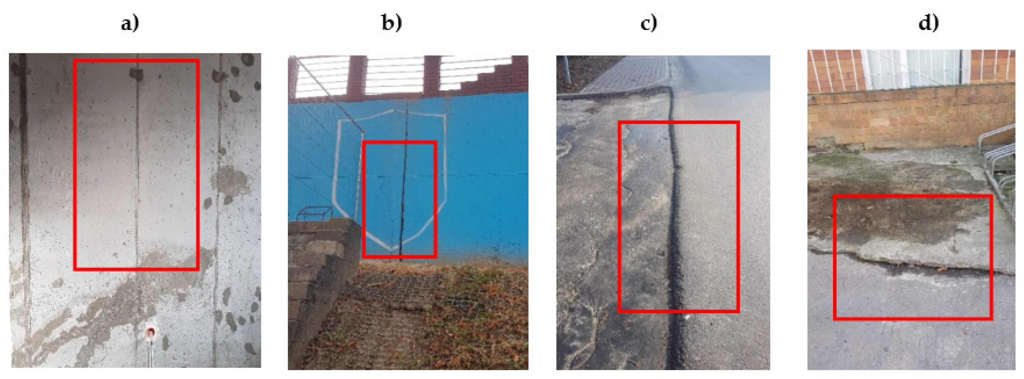
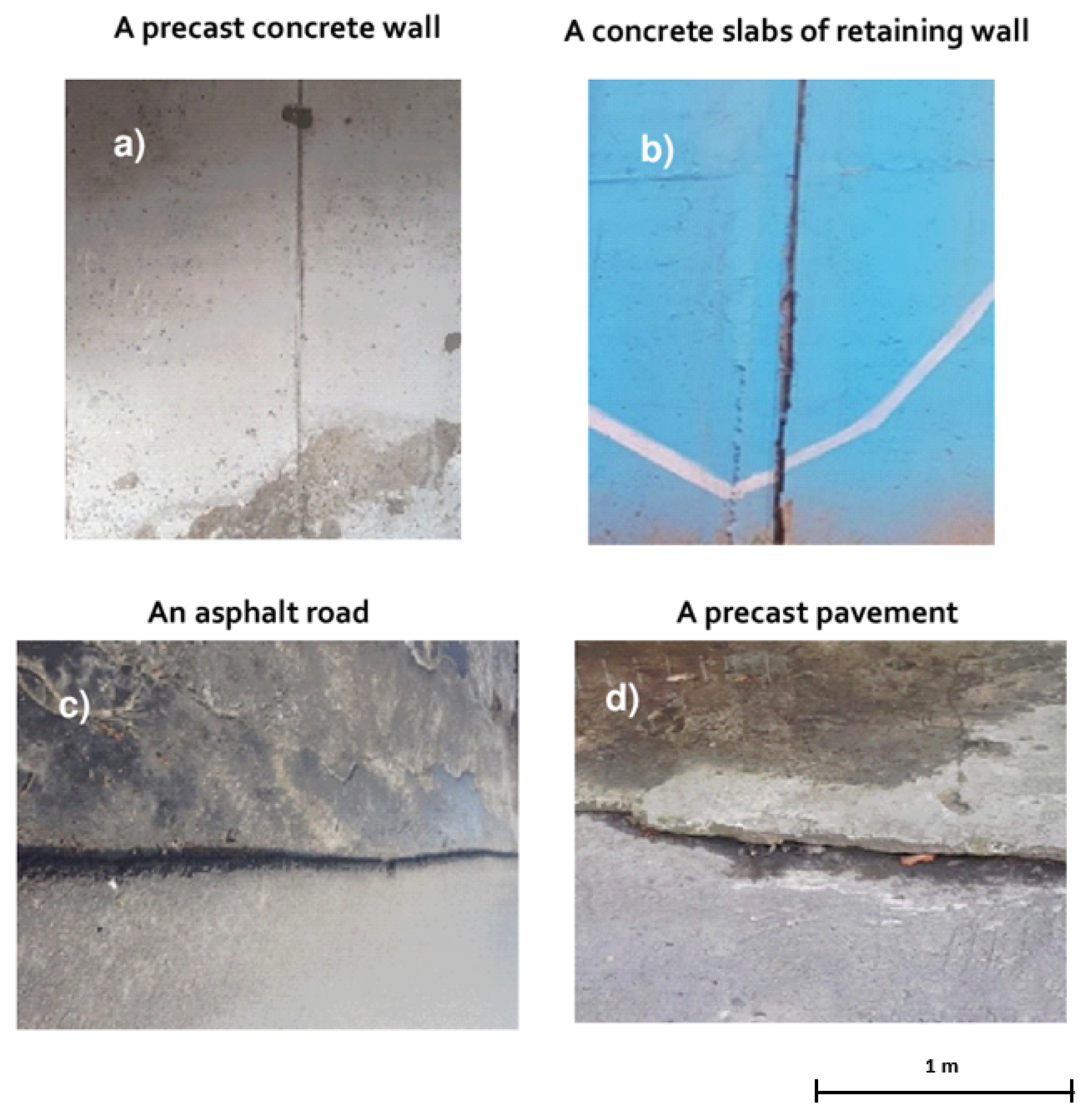
The test measurements were performed using a Leica ScanStation C-10 scanner. The Leica C-10 scanner is based on the time-of-flight principle. The measurements were performed for four different objects. These objects are illustrated in Figure 3 and Figure 4. Figure 3 presents photos of the objects and the areas of study (marked with a red rectangle) that have been fitted using the Msplit estimation method. Figure 4 presents the areas of study, which have been enlarged and corresponds to the clouds of the points shown in Figure 5. Two objects (a,b) represent vertical planes (V), and another two objects (c,d) are horizontal planes (HZ). Figure 3a presents a fragment of the wall in a newly built residential building, which was built from prefabricated elements (large concrete slabs). Thus, it is an example of a smooth surface (Figure 3a) built from two concrete prefabricates, on which no displacements were observed.
Figure 3b presents a fragment of a fence built from concrete slabs that are displaced relative to another concrete slab due to landslides caused by heavy rainfall. This object is an example of a clear displacement of two concrete slabs. The size of a crack between the displaced elements is about 7 cm (see Figure 3b).
The third object is an example of a horizontal shift. Figure 3c shows a fragment of a freshly renovated road. In Figure 3c, one can see a new asphalt layer laid only on one section of a road; hence, there is a large defect between the street with the new asphalt layer and the one that does not have a new layer. Figure 3d presents a fragment of pavement. The pavement is damaged, and the displacement of its fragments is visible. This example differs from object 3 because surface roughness can be also observed. The choice of two such objects, such as those in Figure 3c,d, is intentional. The object in Figure 3c has a smoother, more uniform structure, compared to the concrete pavement with a jagged edge and numerous defects. The structure of the object in Figure 3d is very diverse and rough, and it has numerous depressions.
Such surface examples were selected for testing to check in which cases it will be possible to fit two planes into a set of points constituting one-point cloud using the Msplit estimation method.
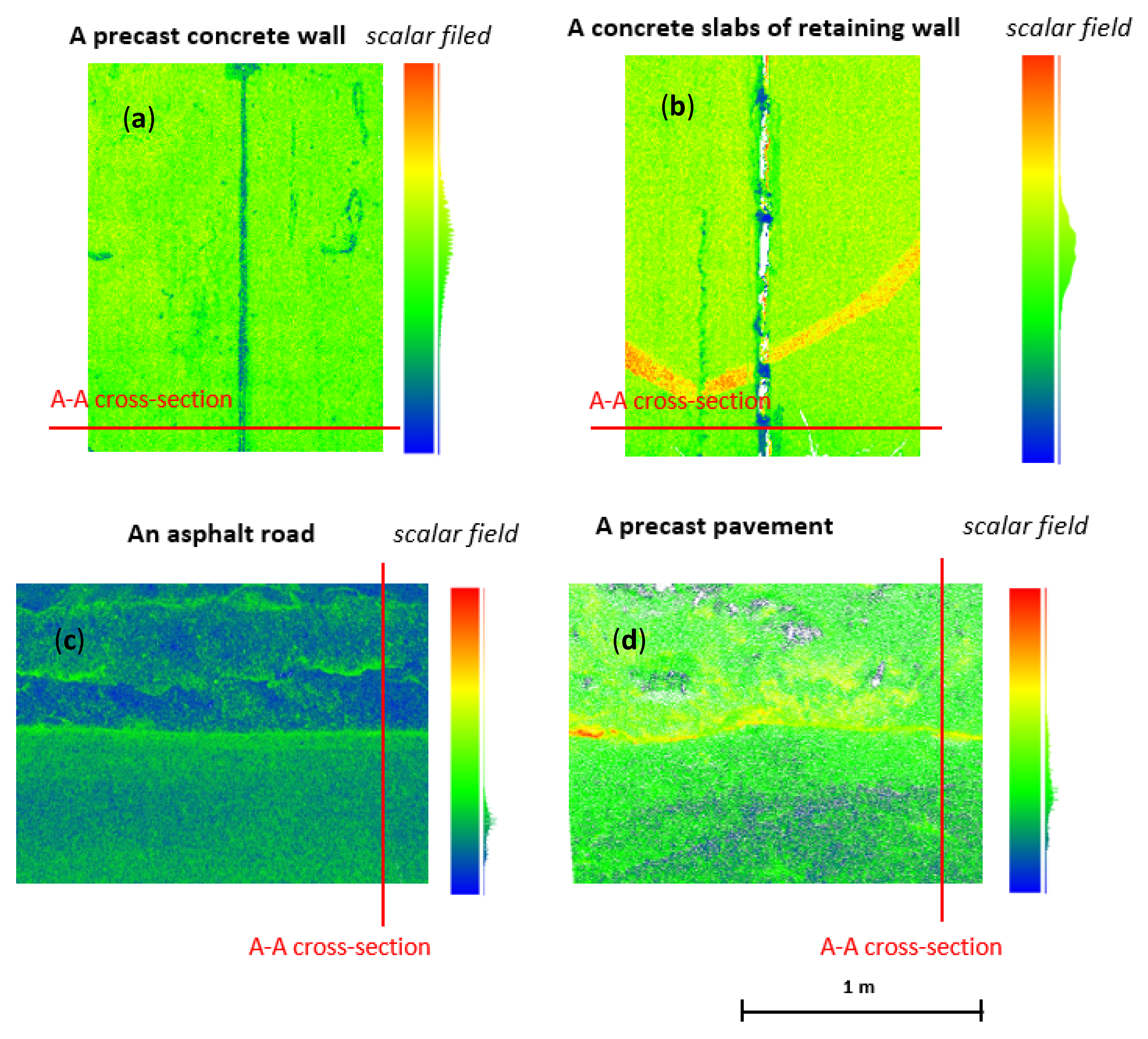
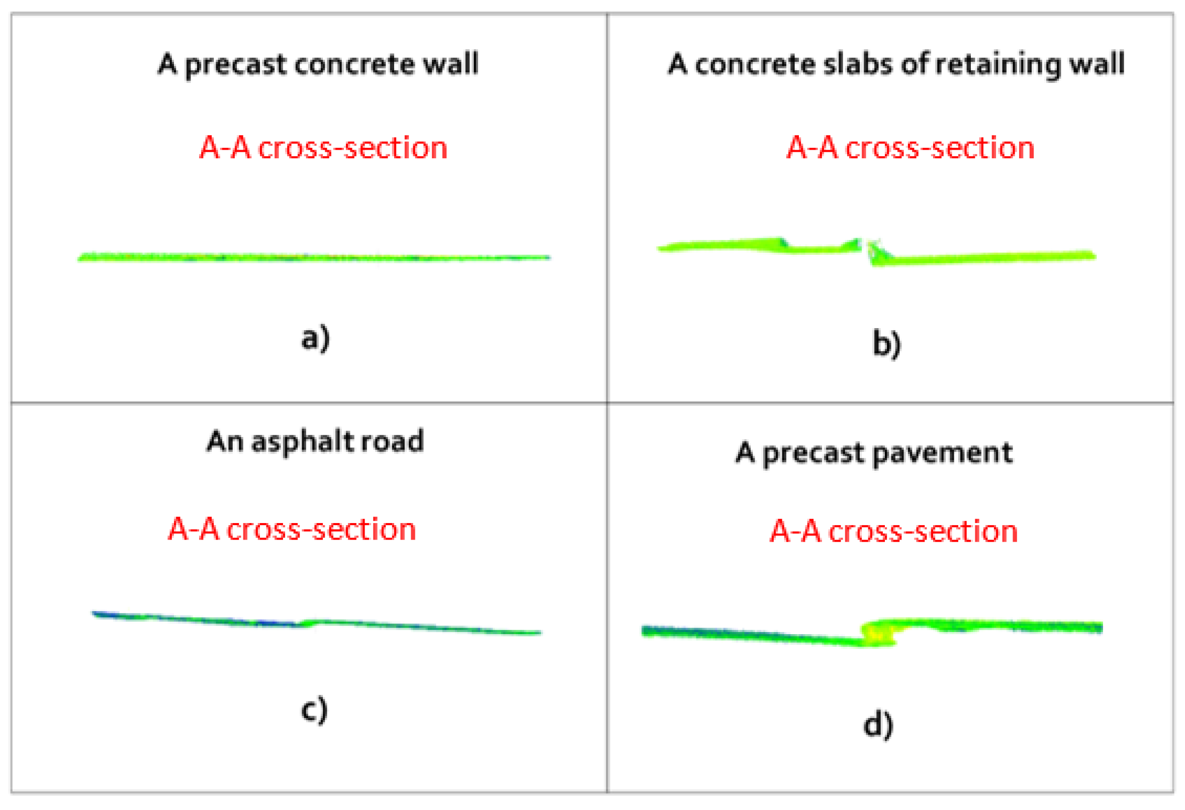
Each object presented in Figure 3 was measured with a 5 mm resolution. As a result of the measurements, point clouds were obtained (see Figure 5). Figure 6 shows the cross-section of each point cloud through the A-A line. It can be observed that the adjacent planes of the objects in Figure 6a,c do not show a height difference. These planes seem to create one plane, while Figure 6b,d clearly form two surfaces.

2.3. Software Description

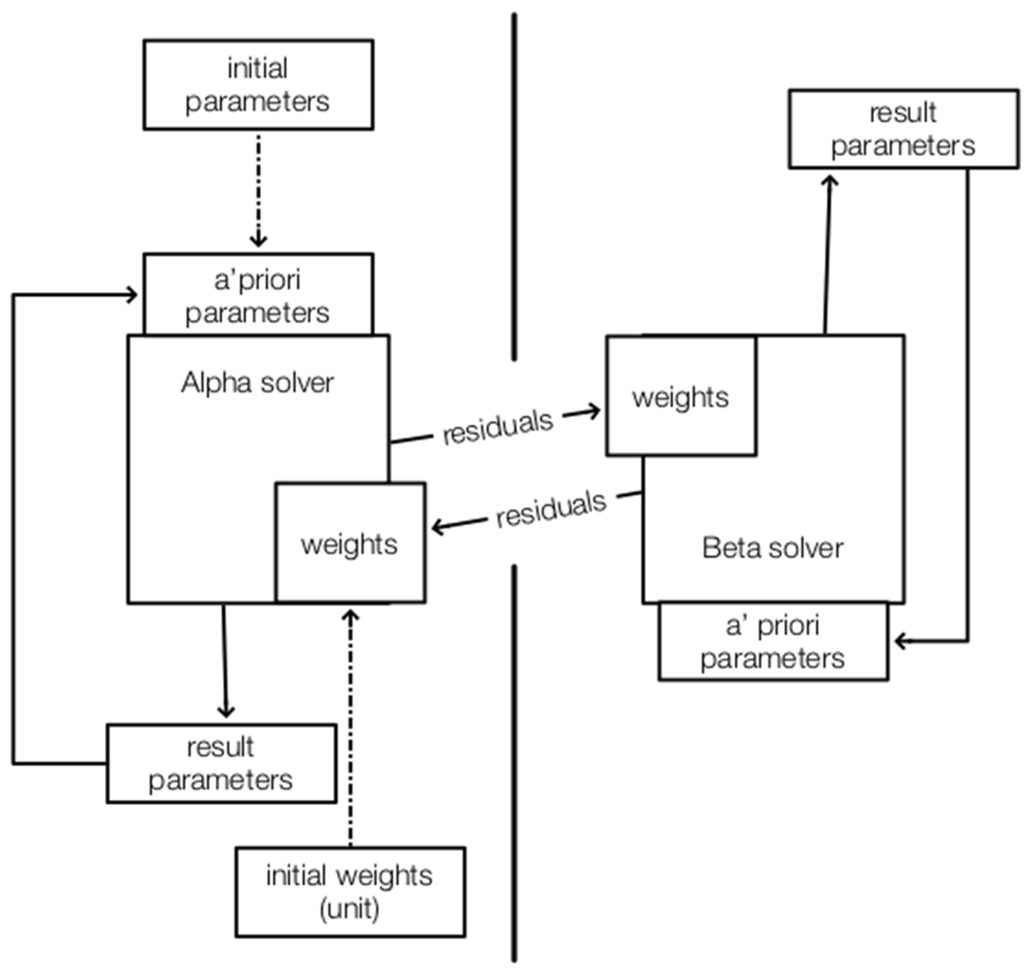
To perform calculations and to fit planes into the point cloud, our own software was used. The algorithm proposed by the authors implements the Msplit estimation method. In the Msplit estimation process, the parameters of two planes α and β are estimated. To achieve this task, the cross-weighting procedure is performed. The first step is called α-solution. Based on the alpha parameters, the alpha residuals are calculated. Then, the beta weights ( ω β ) of observation are modified according to Equation (4). The parameters and free terms are updated. In the next step, the second β-solution is calculated using the least-squares method. The new weights for the α-solution ( ω α ) are calculated. Then, the procedure returns to the α-solution, and the process is iteratively repeated until the increase of the estimated parameters reaches the iteration end threshold. The procedure is shown in Figure 7.
Thus, using the idea of Msplit estimation, the planes were fitted into the point cloud obtained as a result of the measurements performed using a terrestrial laser scanner. In the discussed cases, the Msplit estimation was limited to splitting the functional model into two models.

3. Results

Firstly, all point clouds from four measurement campaigns were imported into the dedicated Leica Cyclon software. Then, the area under consideration was selected and exported from Leica format to a *ptx file, because this is a commonly used format for exchanging scan datasets between different types of software, and it is also the format accepted by our software. The next step was to upload the *ptx files into the software. Because point clouds are large datasets, the software has an option, allowing for the selection of the number of points to fit the planes. A random sampling of point cloud was used in an algorithm to reduce the size of the data set. Processing full datasets significantly extend the processing time.

3.1. The Results of Vertical Object Fitting

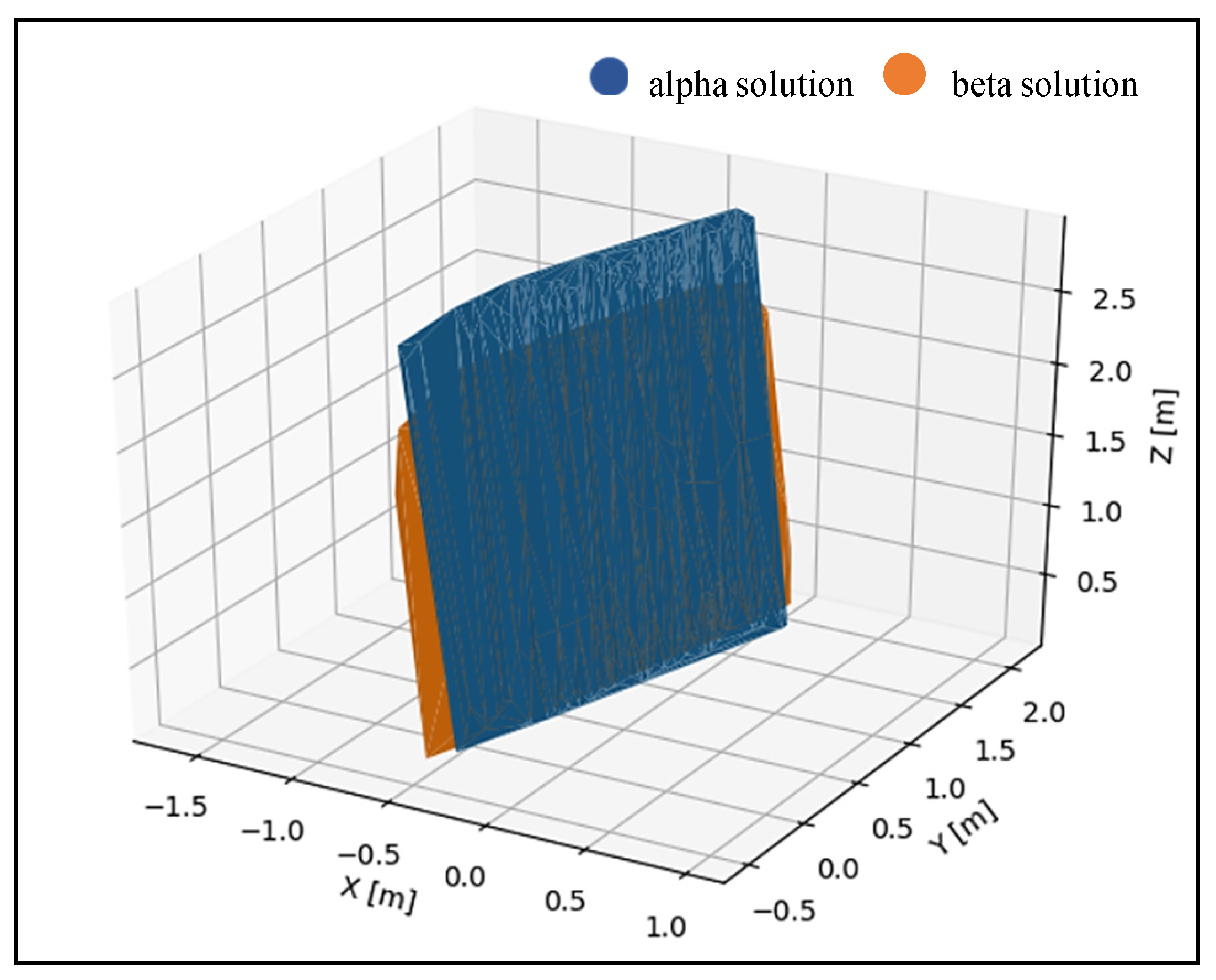
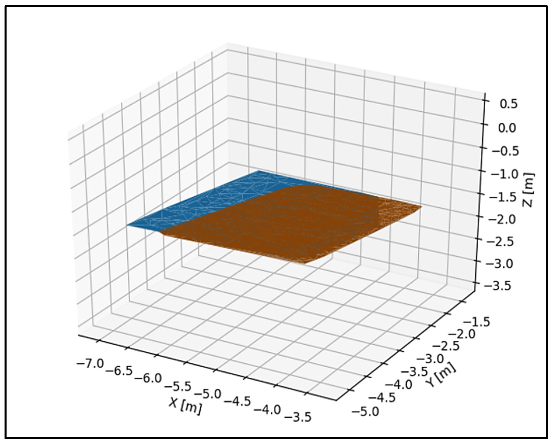
According to the presented algorithm, calculations were performed. The results obtained are presented below in Figure 8 and Figure 9. This section presents the result of fitting two vertical objects: the wall in the building and the retaining wall. As can be observed in Figure 8, the alpha and beta solution overlap. This may indicate that the two planes of the concrete slabs of a wall form a uniform plane, without any displacements.
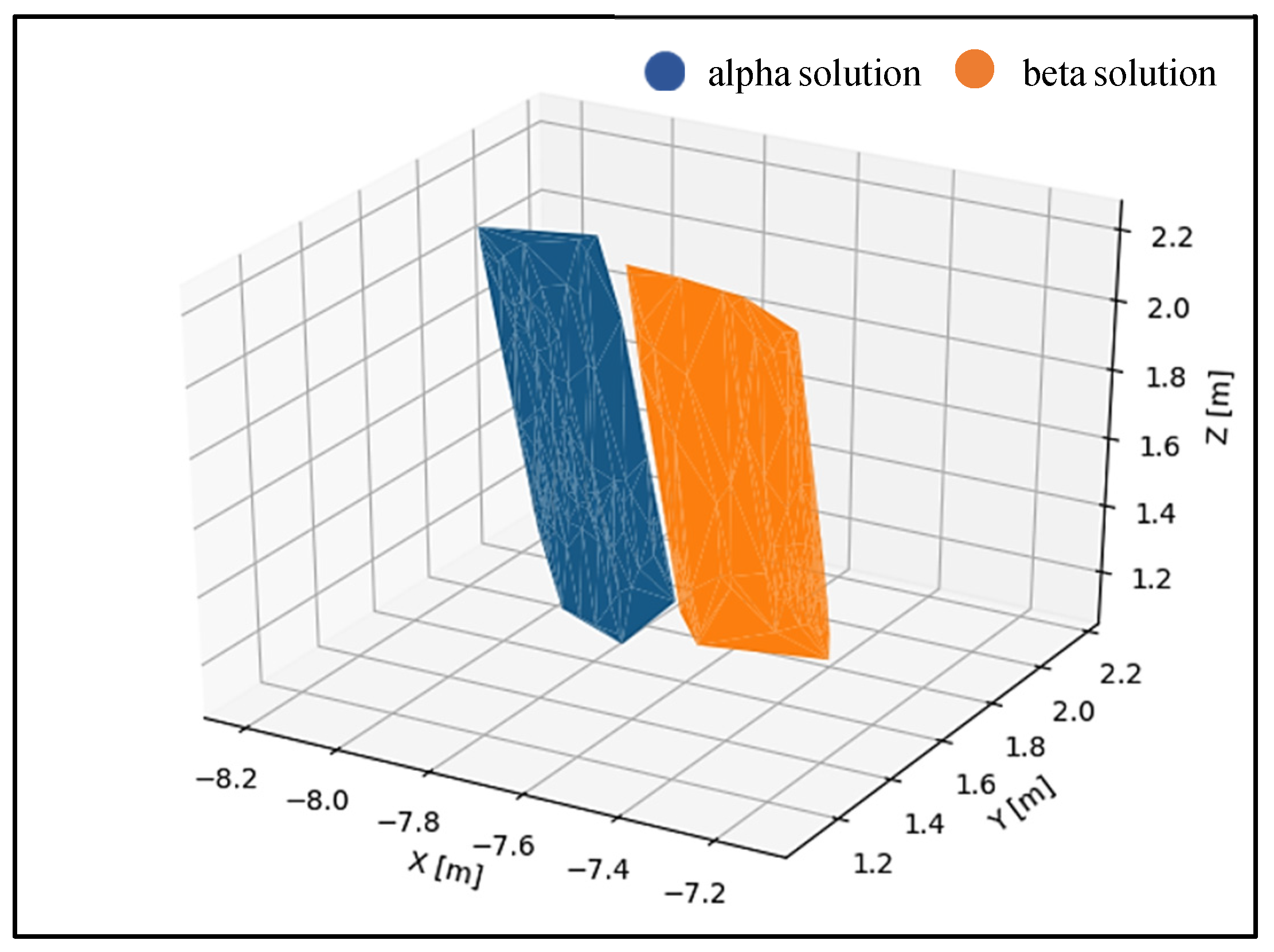
Figure 9 shows an example where displaced wall elements (two plates) were recognized in the dataset, and as a result, two planes (alpha and beta) were fitted into one-point cloud.

3.2. The result of Horizontal Plane Fitting

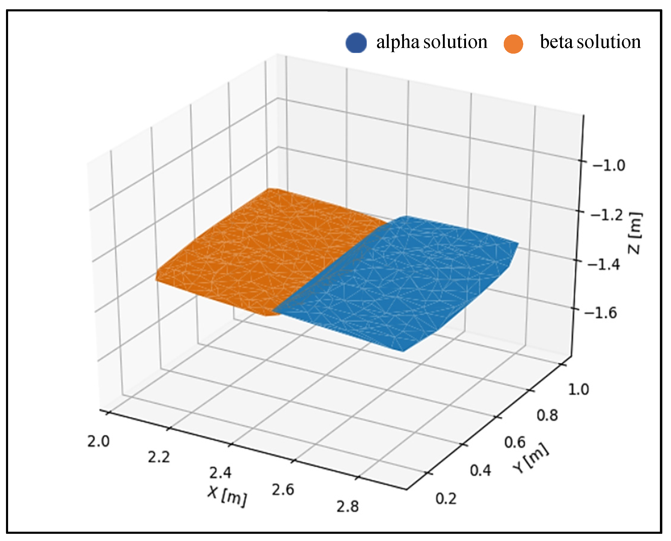
This subsection presents the result of the fitting of two horizontal objects: an asphalt road and a concrete pavement. As in the previous section, the tests performed show two types of solutions. One example is a solution in which the algorithm recognized the displacement of two planes relative to each other (Figure 10). The asphalt road is an example, where the difference between the two elements forming the object was negligible, and the two overlapping planes were defined (Figure 11). This might also indicate that the parameters of these planes are very similar.

3.3. Residual Characteristics

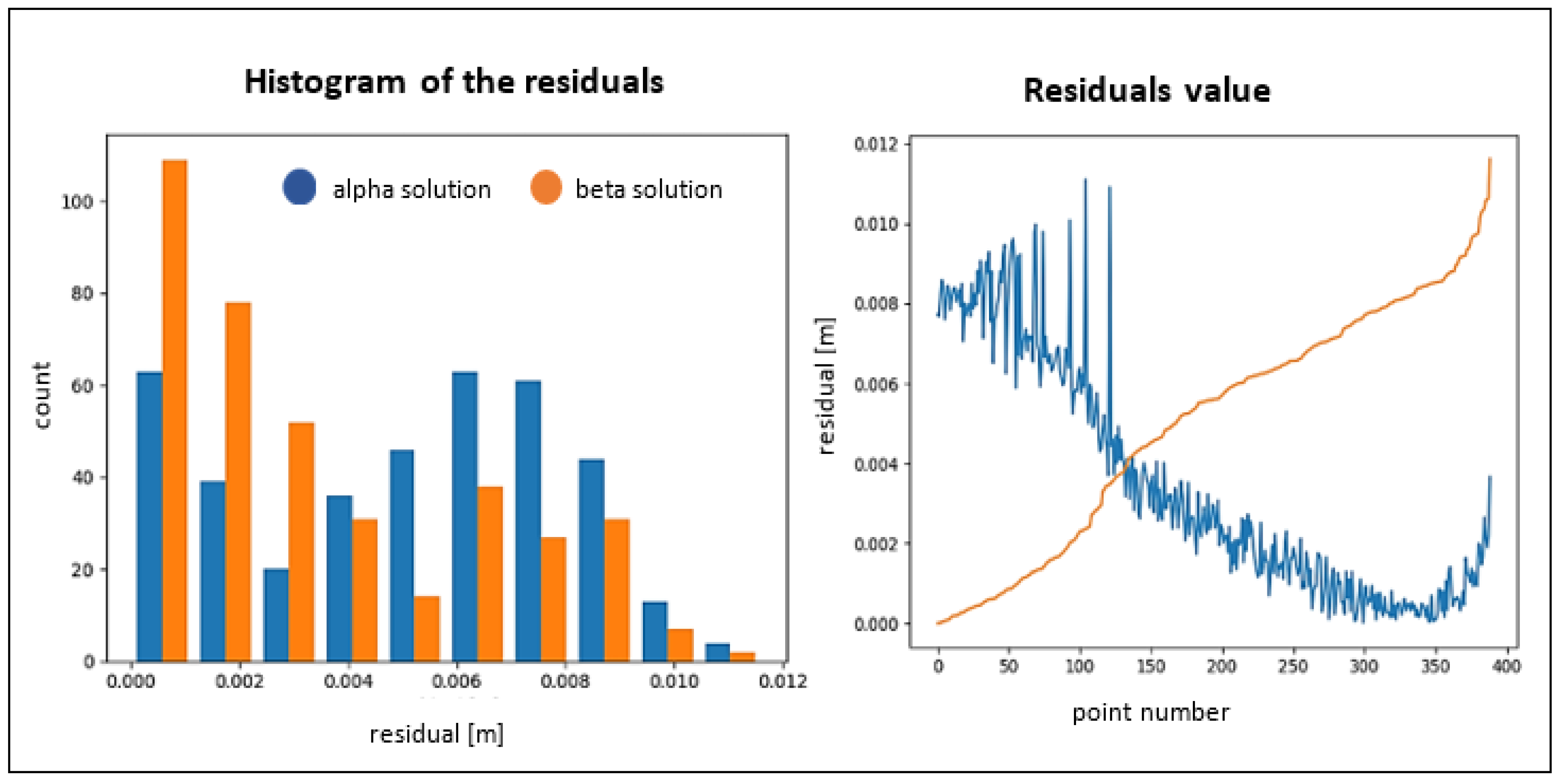
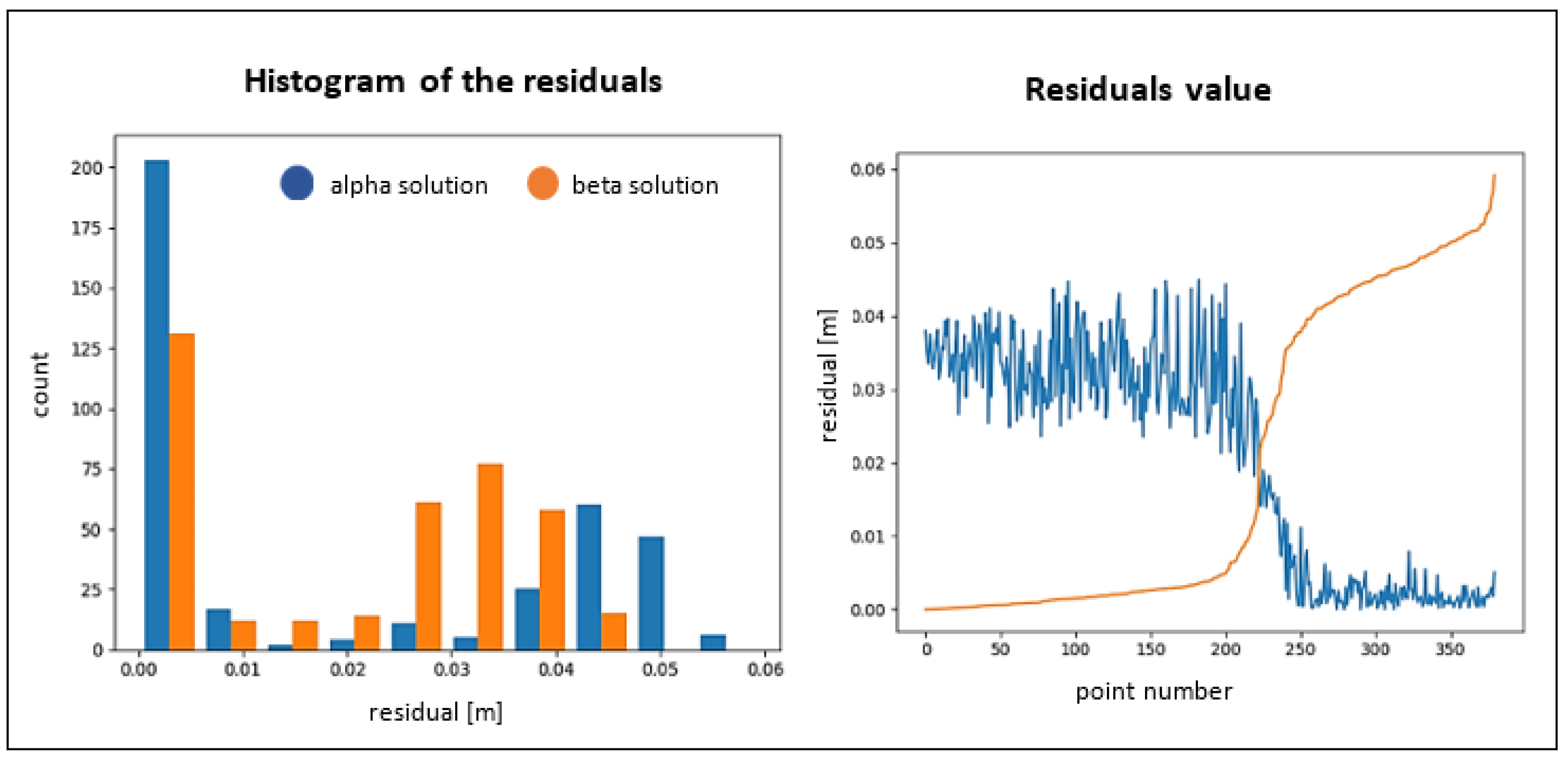
The goal of the conducted research was to indicate the usefulness of the Msplit estimation method in identifying two planes in one-point cloud. The datasets from terrestrial laser scanning were used for this purpose. The conducted research proved that Msplit estimation allows for the extraction of displaced planes if these planes differ in their parameters. Histograms of the residuals and the value of the residuals are presented in Figure 12, Figure 13, Figure 14 and Figure 15.
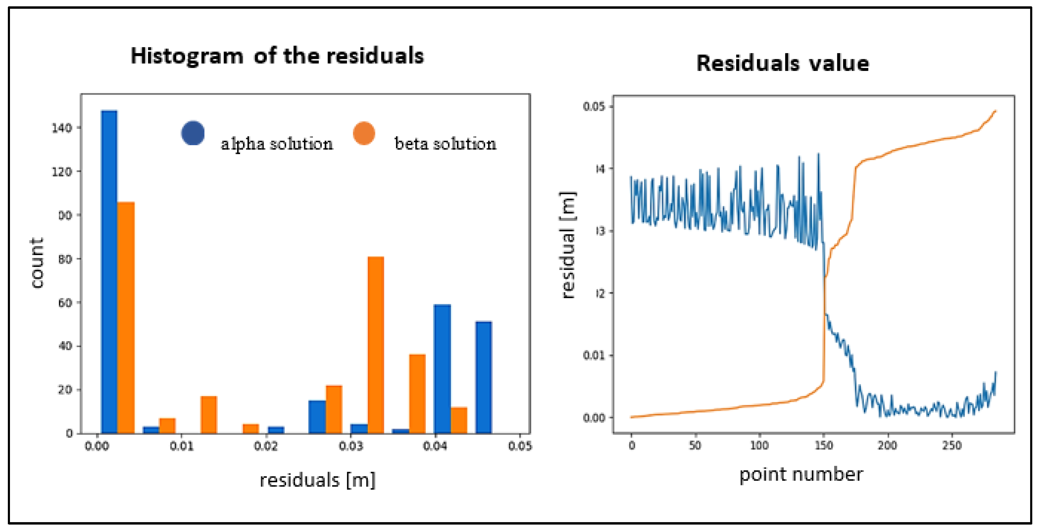
The histogram of the residuals presents the values obtained for the alpha and beta solutions. It can be observed, in Figure 12, that the values of the residuals do not exceed 1 cm for both solutions. The “residual values” graph shows the relation between the points belonging to each solution. If in the point cloud, the Msplit algorithm recognizes two planes with different parameters, then a clear breakpoint should be visible (the blue and orange lines would look like they do in Figure 13). In Figure 12, this trend is not observed, which means that the algorithm did not define the two different planes.
Figure 13 presents the residuals value obtained for each solution (alpha and beta), and one can see that they do not exceed 0.05 m for both solutions (histogram of the residuals). The “residual values” graph presents the distribution of the residuals for the alpha and beta solutions. It can be observed that the residuals from point numbers 1–150 (orange color) do not exceed 0.01 m, while the residuals marked in blue in the range of point numbers 1–150 are about 0.03–0.04 m. The opposite situation is in the range of point numbers 150–300 (blue color line). This means that points 1–150 have been assigned to the beta plane, and points 150–300 have been assigned to the alpha plane.
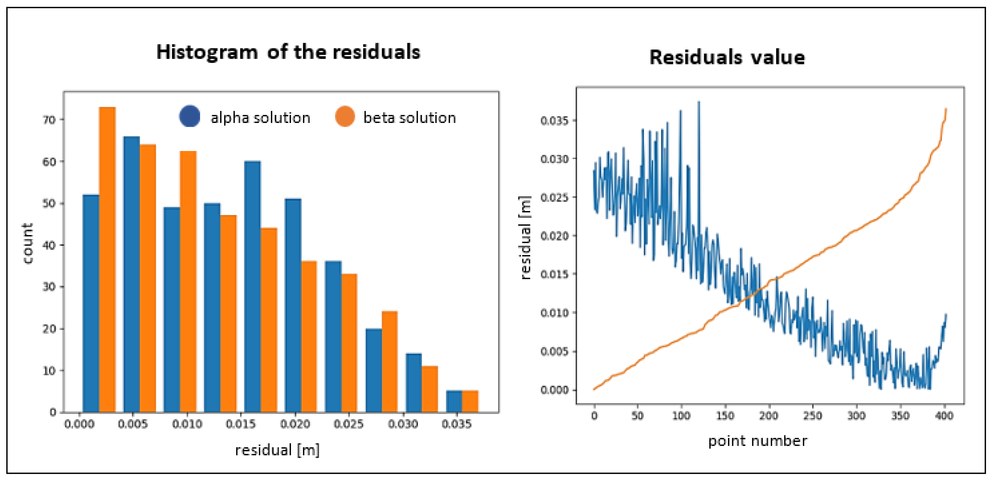
Figure 14 and Figure 15 show the characteristics of the residuals obtained for the two horizontal datasets. The next two examples should be interpreted based on Figure 12 and Figure 13. In Figure 14, a breakpoint between the two solutions cannot be observed. A blue line with a decreasing trend and an orange line with a rising trend is observed. The opposite is the case in Figure 15, where you can see a clear division into two solutions: alpha and beta. The Msplit algorithm assigned about 220 points to the beta solution and about 120 points to the alpha solution.
Based on the “residual values” graph in Figure 15, it can be observed that the residuals from point number 1 to about point number 220 (orange color) do not exceed 0.015 m, while the residuals marked in blue in the range of point numbers 1–220 are about 0.04 m.
The opposite situation is in the range of point numbers 220 to 360 (blue color line). This means that points 1–220 have been assigned to the beta plane, and points 220–360 have been assigned to the alpha plane.
Root mean square (RMS) values were calculated for each plane fitting (Table 1). In each case, the RMS value for both the α and β solutions are similar, which points to the conclusion that the two planes in each object were extracted, and no other planes or outliers are present in the point cloud. The distribution of points relative to the fitted planes in each of the four presented objects is even. Table 2 shows the plane parameters received for each object in the α and β solution.
Comparing the received parameters a 0 α ,   a 1 α , a 2 α , z α and a 0 β ,   a 1 β ,   a 2 β ,   z β it can be observed that “Precast concrete wall” and “An asphalt road” objects are characterized by similar parameters while “Retaining wall” and “Precast pavement” parameters in α solution and β solution differ.
Table 3 presents an efficiency analysis for the calculation time and the obtained RMS values for the alpha and beta solutions. The parameters were calculated for different variants depending on the percentage reduction of the data set.

3.4. The Result of Msplit(q) Estimation Fitting and Residual Characteristic

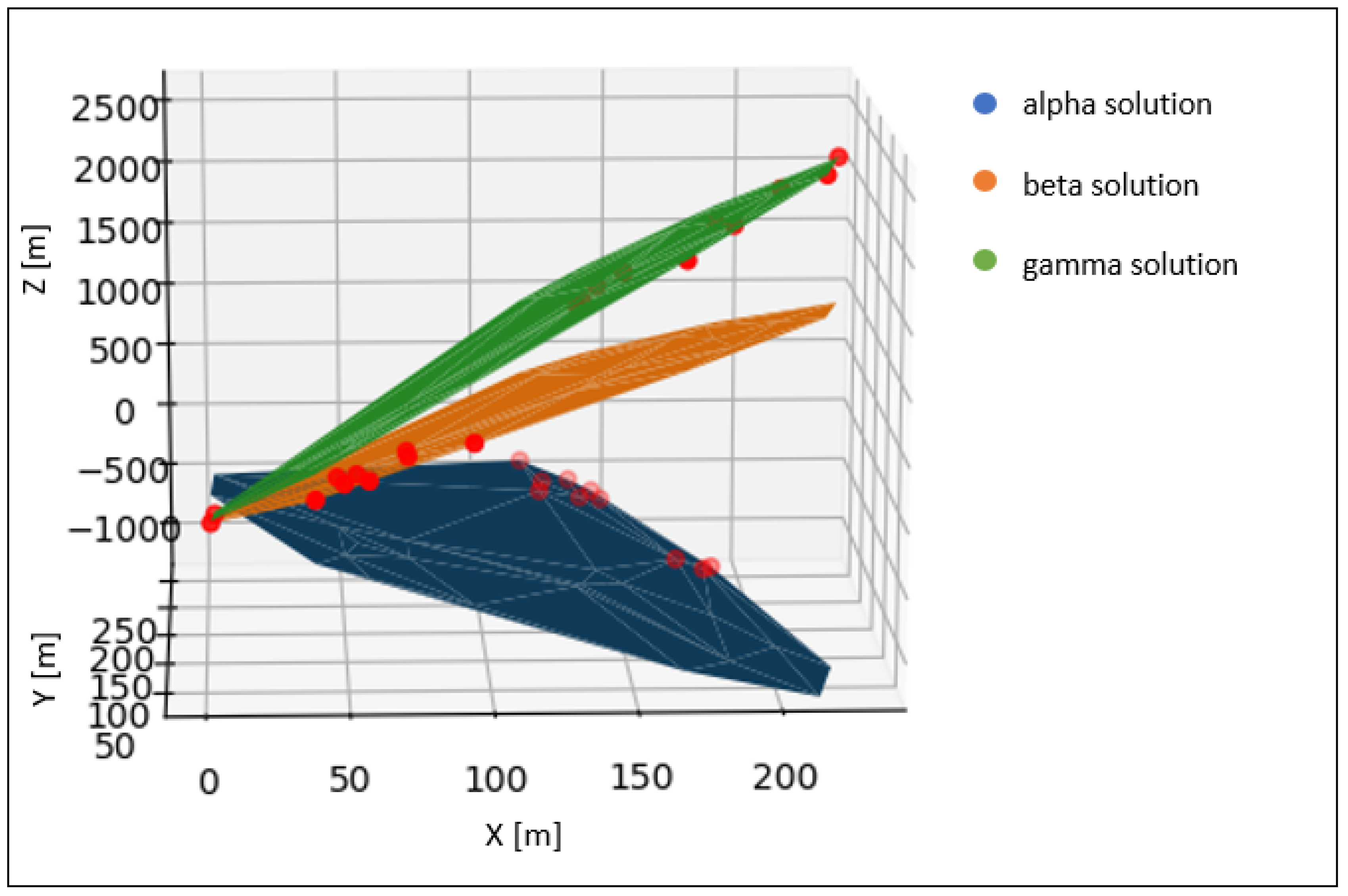
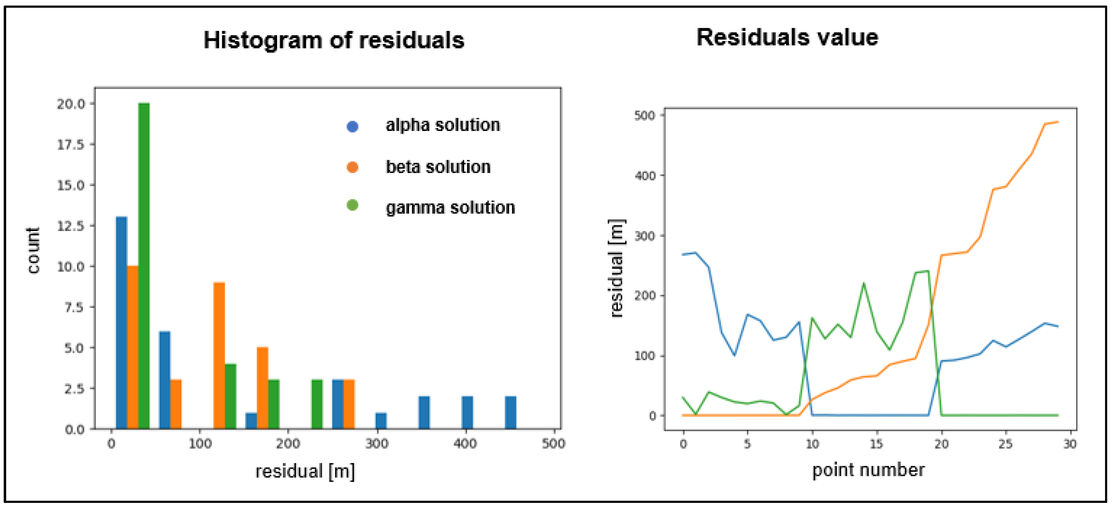
This subsection presents the result of the three planes fitting. The planes were generated as test objects and the Msplit(q) fitting results are presented in Figure 16. Based on the assumption that we want to obtain three planes, points were generated to meet this condition. Then a data file was created containing the XYZ coordinates of these 30 points. In the next step, according to the Msplit(q) estimation algorithm discussed in Section 2.1.2, the assumed planes were fitted.
The histogram of the residuals presents the values obtained for the alpha, beta, and gamma solutions. These three planes have been generated therefore the residuals value differs from the real objects results. It can be observed that points 1–10 belong to the alpha plane, 11–20 to the beta plane, and 21–30 to the gamma plane, it is indicated by the “residuals value” presented in Figure 17.

4. Discussion

This paper applied the Msplit method of estimation to fit two planes into one-point cloud. This approach is possible when the analyzed object or its elements can be described using mathematical functions. In the examples considered in this study, the authors focused on planes. The inspiration was a real situation that recently occurred after heavy rain. Rainwater washed the ground, and as a result, a retaining wall moved. Concrete slabs constituting elements of the wall displaced in relation to each other. One of the options was to measure this wall using a terrestrial laser scanner to estimate the extent of the damage. While processing the point cloud, the idea arose to identify the different planes contained in one-point cloud. The overarching assumption was that the use of the Msplit estimation method was suitable for processing a point cloud.
The efficacy of the Msplit method has been confirmed by tests carried out on different datasets. The sensitivity of the proposed method was described by the authors of this method in [27]. The size of the displacement is an important issue here. To split the functional model into at least two models, these models must be described by different parameters. This means that the planes must be distinguishable in a point cloud measured with TLS. However, the situation can also be interpreted so that if they do not split the model into two (or more, depending on the situation), it can be said that there was no displacement. This situation is shown in Figure 3a (the precast concrete wall of an apartment in a multi-story building in a developer state).
The development of point clouds covering individual walls built from concrete slabs or blocks using the Msplit estimation method in a short time allowed an opinion to be formed regarding the quality of the construction process. Figure 4a shows a fragment of a wall (in one of the apartments) consisting of two concrete slabs. As a result of the study, no displacement of the planes relative to other planes was observed. The algorithm fitted one plane into the entire point cloud, as shown in Figure 8. Thus, it can be concluded that there are no significant displacements that may affect the condition of the structure.
The second vertical object is a retaining wall built from concrete slabs. This object is a good example of using Msplit estimation to fit two planes into a point cloud representing a vertical object whose elements have been displaced. Figure 9 clearly shows the two planes into which the functional model was split.
The next two examples are horizontal surfaces. Additionally, these examples confirm the effectiveness of the proposed estimation method. Figure 10 and Figure 11 present the results of the fitting.
When using the proposed method, it should be remembered that, depending on whether they are of horizontal or vertical planes, functional models should be properly formulated. A functional model must be selected very carefully and based on a mathematical description of the estimated model and data structure.

5. Conclusions

Msplit estimation can be successfully applied in the detection of two planes. It allows a dataset to be correctly split into two and the planes to be fitted to the appropriate dataset. In the solution proposed by the authors, tests were carried out to split the functional model into two. Further testing will be performed for more than two models.
If a displacement does not occur, Msplit estimation cannot split the functional model nor detect two planes with different parameters. Finally, as a result, two overlapping planes were fitted (see “precast concrete wall” and “an asphalt road”). In addition, both horizontal and vertical surfaces, measured with a terrestrial laser scanner, can be analyzed using Msplit estimation.

Author Contributions

Conceptualization, J.J.; methodology, J.J. and J.R.; software, J.R.; investigation, J.J.; resources, J.J. and J.R.; data curation, W.B-B.; writing—original draft preparation, J.J.; writing—review and editing, W.B.-B. and C.S.; visualization, J.J.; All authors have read and agreed to the published version of the manuscript.

Funding

This research received no external funding.

Conflicts of Interest

The authors declare no conflict of interest.

References

  1. Kaloop, M.R.; Beshr, A.A.; Elshiekh, M.Y. Using Total Station for monitoring the deformation of high strength concrete beams. In Proceedings of the 6th International Conference on Vibration Engineering (ICVE), Dalian, China, 6–9 June 2008. [Google Scholar] [CrossRef]
  2. Mrówczyńska, M.; Gibowski, S. Indicating Vertical Deviation of Historical Buildings Using Geodetic Methods—Case Study of Brick and Wood Tower in Nowe Miasteczko. Civ. Environ. Eng. Rep. 2016, 22, 127–136. [Google Scholar] [CrossRef] [Green Version]
  3. Mrówczyńska, M. Analysis of the horizontal structure of a measurement and control geodetic network based on entropy. Geod. Cartogr. 2013, 62, 23–31. [Google Scholar] [CrossRef]
  4. Khalil, A.M. Two-dimensional displacement measurement using static close range photogrammetry and a single fixed camera. Alex. Eng. J. 2011, 50, 219–227. [Google Scholar] [CrossRef] [Green Version]
  5. Brown, C.J.; Karuna, R.; Ashkenazi, V.; Roberts, G.W.; Evans, R.A. Monitoring of structures using the Global Positioning System. Proc. Inst. Civ. Eng. Struct. Build. 1999, 134, 97–105. [Google Scholar] [CrossRef]
  6. Kovačič, B.; Kamnik, R.; Premrov, M.; Gubeljak, N.; Predan, J.; Tišma, Z. Modern deformation measurement techniques and their comparison. Stroj. Vestn. J. Mech. Eng. 2008, 5, 364–371. [Google Scholar]
  7. Suchocki, C.; Błaszczak-Bąk, W. Down-Sampling of Point Clouds for the Technical Diagnostics of Buildings and Structures. Geosciences 2019, 9, 70. [Google Scholar] [CrossRef] [Green Version]
  8. Błaszczak-Bąk, W.; Suchocki, C.; Janicka, J.; Dumalski, A.; Duchnowski, R.; Sobieraj-Żłobińska, A. Automatic threat detection for historic buildings in dark places based on the modified OPTD method. ISPRS Int. J. Geo-Inf. 2020, 9, 123. [Google Scholar] [CrossRef] [Green Version]
  9. Rodríguez-Gonzálvez, P.; Fernández-Palacios, B.J.; Muñoz-Nieto, A.L.; Arias-Sanchez, P.; Gonzalez-Aguilera, D. Mobile LiDAR system: New possibilities for the documentation and dissemination of large cultural heritage sites. Remote Sens. 2017, 9, 189. [Google Scholar] [CrossRef] [Green Version]
  10. Rüther, H.; Chazan, M.; Schroeder, R.; Neeser, R.; Held, C.; Walker, S.J.; Matmon, A.; Horwitz, L.K. Laser scanning for conservation and research of African cultural heritage sites: The case study of Wonderwerk Cave, South Africa. J. Archaeol. Sci. 2009, 36, 1847–1856. [Google Scholar] [CrossRef]
  11. Pawłowicz, J.A. Importance of Laser Scanning Resolution in the Process of Recreating the Architectural Details of Historical Buildings. In Proceedings of the IOP Conference Series: Materials Science and Engineering, Sibiu, Romania, 14–17 June 2017. [Google Scholar]
  12. Suchocki, C. Application of terrestrial laser scanner in cliff shores monitoring. Rocz. Ochr. Sr. 2009, 11, 715–725. [Google Scholar]
  13. Janowski, A.; Szulwic, J.; Tysiac, P.; Wojtowicz, A. Airborne and mobile laser scanning in measurements of sea cliffs on the Southern Baltic. In Proceedings of the International Multidisciplinary Scientific GeoConference Surveying Geology and Mining Ecology Management (SGEM), Albena, Bulgaria, 18–24 June 2015. [Google Scholar]
  14. Li, J.; Wan, Y.; Gao, X. A new approach for subway tunnel deformation monitoring: High-Resolution terrestrial laser scanning. ISPRS Int. Arch. Photogramm. Remote Sens. Spat. Inf. Sci. 2012, 39, 223–228. [Google Scholar] [CrossRef] [Green Version]
  15. Suchocki, C.; Jagoda, M.; Obuchovski, R.; Šlikas, D.; Sužiedelytė-Visockienė, J. The properties of terrestrial laser system intensity in measurements of technical conditions of architectural structures. Metrol. Meas. Syst. 2018, 25, 779–792. [Google Scholar]
  16. Błaszczak-Back, W.; Suchocki, C.; Janicka, J.; Dumalski, A.; Duchnowski, R. Defect detection of historic structures in dark places based on the point cloud analysis by modified OptD method. Int. Arch. Photogramm. Remote Sens. Spat. Inf. Sci. 2019, XLII-3/W8, 71–77. [Google Scholar] [CrossRef] [Green Version]
  17. Corso, J.; Roca, J.; Buill, F. Geometric analysis on stone façades with terrestrial laser scanner technology. Geoscience 2017, 7, 103. [Google Scholar] [CrossRef] [Green Version]
  18. Janowski, A.; Rapinski, J. M-Split Estimation in Laser Scanning Data Modeling. J. Indian Soc. Remote Sens. 2013, 41, 15–19. [Google Scholar] [CrossRef]
  19. Wang, C.K.; Hsu, P.H. Building Detection and Structure Line Extraction from Airborne LiDAR Data. Building 2007, 12, 365–379. [Google Scholar]
  20. Zheng, J.; Mccarthy, T.; Fotheringham, A.S.; Yan, L. Linear Feature Extraction of Buildings from Terrestrial LIDAR Data with Morphological Techniques. Int. Arch. Photogramm. Remote Sens. Spat. Inf. Sci. 2008, 37, 241–244. [Google Scholar]
  21. Wiśniewski, Z. Estimation of parameters in a split functional model of geodetic observations (Msplit estimation). J. Geod. 2009, 83, 105–120. [Google Scholar] [CrossRef]
  22. Błaszczak-Bąk, W.; Janowski, A.; Kamiński, W.; Rapiński, J. Application of the Msplit method for filtering airborne laser scanning data-sets to estimate digital terrain models. Int. J. Remote Sens. 2015, 36, 2421–2437. [Google Scholar] [CrossRef]
  23. Janicka, J. Transformation of coordinates with robust M-estimation and modified Hausbrandt correction. In Proceedings of the 8th International Conference on Environmental Engineering (ICEE), Vilnius, Lithuania, 19–20 May 2011; pp. 1330–1333. [Google Scholar]
  24. Wyszkowska, P.; Duchnowski, R. Performance of Msplit estimates in the context of vertical displacement analysis. J. Appl. Geod. 2020, 14, 149–158. [Google Scholar] [CrossRef]
  25. Janowski, A. The circle object detection with the use of Msplit estimation. E3S Web Conf. 2018, 26, 00014. [Google Scholar] [CrossRef] [Green Version]
  26. Wiśniewski, Z. Msplit(q) estimation: Estimation of parameters in a multi split functional model of geodetic observations. J. Geod. 2010, 84, 355–372. [Google Scholar] [CrossRef]
  27. Wiśniewski, Z.; Duchnowski, R.; Dumalski, A. Efficacy of Msplit estimation in displacement analysis. Sensors 2019, 19, 5047. [Google Scholar] [CrossRef] [Green Version]
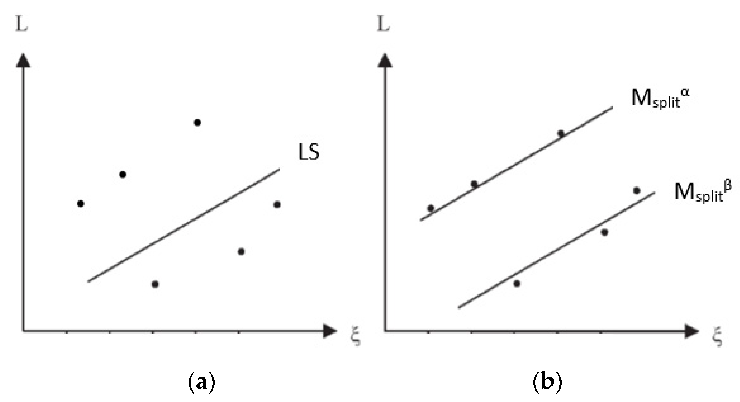
Figure 1. The idea of Msplit estimation and the least-squares method, with the example of line fitting. Figure 1 shows a line fit using the least-squares method (a) and Msplit estimation (b). Similarly, one can fit two or more planes into a set of points by splitting the functional model into two or more, respectively.
Remotesensing 12 03203 g001
Figure 2. The idea of Msplit(q) estimation and the Least Square method, with the example of line fitting. Figure 2 shows (a) an observation set, (b) a line fit using the least-squares method, and (c) Msplit(q) estimation.
Remotesensing 12 03203 g002
Figure 3. Photos of the objects and areas of study (marked with a red rectangle) (a) a precast concrete wall, (b) concrete slabs of retaining wall, (c) an asphalt road, (d) a precast pavement.
Remotesensing 12 03203 g003
Figure 4. The fragments of the real objects measured using Terrestrial Laser Scanning (TLS).
Remotesensing 12 03203 g004
Figure 5. Point clouds representing the objects presented in Figure 2 (ad, respectively).
Remotesensing 12 03203 g005
Figure 6. Cross-section view of the point clouds shown in Figure 3, respectively.
Remotesensing 12 03203 g006
Figure 7. Block diagram of Msplit estimation.
Remotesensing 12 03203 g007
Figure 8. Precast concrete wall (Msplit fitting result).
Remotesensing 12 03203 g008
Figure 9. Concrete slabs of a retaining wall (Msplit fitting result).
Remotesensing 12 03203 g009
Figure 10. Concrete pavement (Msplit fitting result).
Remotesensing 12 03203 g010
Figure 11. Asphalt road (Msplit fitting result).
Remotesensing 12 03203 g011
Figure 12. Precast concrete wall.
Remotesensing 12 03203 g012
Figure 13. Concrete slabs of a retaining wall.
Remotesensing 12 03203 g013
Figure 14. Asphalt road.
Remotesensing 12 03203 g014
Figure 15. Concrete pavement.
Remotesensing 12 03203 g015
Figure 16. Test object—Msplit(q) fitting.
Remotesensing 12 03203 g016
Figure 17. Test object histogram of residuals and residuals value.
Remotesensing 12 03203 g017
Table 1. RMS values for the α solution and β solution and percentage of points in the planes α and β, respectively.
Object NameRMSα plane [m]RMSβ plane [m]α Planeβ Plane
A precast concrete wall0.00580.004535%65%
A retaining wall0.02870.024653%47%
An asphalt road0.01660.015646%54%
A precast pavement0.02870.025757%43%
Table 2. Plane parameters respectively for the α solution and β solution.
Precast Concrete WallRetaining WallAsphalt RoadPrecast Pavement
α Solutionβ Solutionα Solutionβ Solutionα Solutionβ Solutionα Solutionβ Solution
a 0 α 0.26980.2722−2.0063−2.8107−0.0125−0.01500.03550.0630
a 1 α −0.7130−0.72315.91064.92350.13330.1232−0.0491−0.0378
a 2 α 2.68202.71718.14756.78180.75650.74841.07800.9567
z α 1.10461.09921.26171.11911.51081.44500.63980.5922
Table 3. An efficiency analysis (the computation time and RMS values).
Dataset
100%
Dataset
10%
Dataset
1%
Dataset
0.1%
Precast concrete wallNo. of Points3884389--
T [s]/kB40/17444--
RMSα0.00580.0058--
RMSβ0.00420.0045--
Retaining wallNo. of Points285---
T [s]16/134---
RMSα0.0287---
RMSβ0.0246---
Asphalt roadNo. of Points402219402224022402
T [s]5019/157 082509555
RMSα0.01750.01740.01750.0166
RMSβ0.01520.01520.01520.0156
Precast pavementNo. of Points380003800380-
T [s]702/ 14 094687-
RMSα0.02840.02820.0287-
RMSβ0.02610.02620.0257-