Article

Flood Hazard Risk Mapping Using a Pseudo Supervised Random Forest

1
Department of Geodesy & Geomatics Engineering, University of New Brunswick, Fredericton, NB E3B 5A3, Canada
2
Natural Resource Canada, Ottawa, ON K1S 5K2, Canada
*
Author to whom correspondence should be addressed.
Remote Sens. 2020, 12(19), 3206; https://doi.org/10.3390/rs12193206
Submission received: 19 August 2020 / Revised: 24 September 2020 / Accepted: 26 September 2020 / Published: 1 October 2020
(This article belongs to the Special Issue Geospatial Techniques for Urban Water Management)

Abstract

:
Devastating floods occur regularly around the world. Recently, machine learning models have been used for flood susceptibility mapping. However, even when these algorithms are provided with adequate ground truth training samples, they can fail to predict flood extends reliably. On the other hand, the height above nearest drainage (HAND) model can produce flood prediction maps with limited accuracy. The objective of this research is to produce an accurate and dynamic flood modeling technique to produce flood maps as a function of water level by combining the HAND model and machine learning. In this paper, the HAND model was utilized to generate a preliminary flood map; then, the predictions of the HAND model were used to produce pseudo training samples for a R.F. model. To improve the R.F. training stage, five of the most effective flood mapping conditioning factors are used, namely, Altitude, Slope, Aspect, Distance from River and Land use/cover map. In this approach, the R.F. model is trained to dynamically estimate the flood extent with the pseudo training points acquired from the HAND model. However, due to the limited accuracy of the HAND model, a random sample consensus (RANSAC) method was used to detect outliers. The accuracy of the proposed model for flood extent prediction, was tested on different flood events in the city of Fredericton, NB, Canada in 2014, 2016, 2018, 2019. Furthermore, to ensure that the proposed model can produce accurate flood maps in other areas as well, it was also tested on the 2019 flood in Gatineau, QC, Canada. Accuracy assessment metrics, such as overall accuracy, Cohen’s kappa coefficient, Matthews correlation coefficient, true positive rate (TPR), true negative rate (TNR), false positive rate (FPR) and false negative rate (FNR), were used to compare the predicted flood extent of the study areas, to the extent estimated by the HAND model and the extent imaged by Sentinel-2 and Landsat satellites. The results confirm that the proposed model can improve the flood extent prediction of the HAND model without using any ground truth training data.

Graphical Abstract

1. Introduction

Floods are a devastating natural hazard but are inadequately understood [1] and controlled [2]. Floods cause severe damage to people, their health and properties, city infrastructures, ecological systems, agricultural lands and economic activities [3,4,5]. Global warming, urbanization along rivers and coasts and climate change are causing rapid growth in flood events around the world [6,7] and it is crucial for the public, the emergency management community and decision-makers to have access to an accurate estimation of the flood extent. There are different approaches for flood prediction including (1) hydrodynamic models [8,9,10,11,12,13]; (2) empirical methods [14,15]; (3) simplified conceptual models [16,17]; and more recently (4) machine learning and statistical models [18,19,20,21].
(1) Hydrodynamic models use mathematical equations to simulate fluid motion and usually require high computational power [22]. These models require significant data inputs such as flow discharge, water depth, gravitational acceleration and channel bed slope, to simulate flow in their attempt to replicate flow patterns and estimate flow velocity and spatial extents of inundation. Hydrodynamic models are mainly divided into three categories depending on their dimensionality, 1D, 2D and 3D. 1D models consider the floodplain flow as one-dimensional along the river central line [8,9] and by solving mass and momentum conservation equations, model the flood over a floodplain on multiple cross-sections. In 2D models, an intensive collection of topographical data are used for flood simulation assuming that the third dimension, water depth, is shallow [22]. 2D models are probably the most common approach among hydrodynamic models for flood mapping [22]. Furthermore, 1D/2D solutions are becoming very popular, where the 1D component models flow in the river and 2D flow modeled on the floodplain [23]. 3D hydrodynamic models generate a complex three-dimensional representation of floodplain which is usually regarded unnecessary because of their extensive required parameters and maybe comparable accuracy with 2D models [22]. For modeling more complicated flood events, which occur due to tsunami and dam breaks and require modeling of vertical turbulence and spiral flow, 3D models provide better representation because of their capability in modeling vertical dimensions [24,25]. The higher dimensionality of a model, the more parameters required for flood simulation and longer computation time. In general, hydrodynamic models are extremely complex, have sensitive outputs based on site-specific parameters, require a substantial amount of data and their calibration is costly [26].
(2) Empirical methods generate flood maps mainly using observations which could be obtained through satellite imagery, aerial photography, land survey and so forth. Depending on the credibility and resolution of the observations, empirical methods generate flood maps with varying accuracy and are mainly used as a benchmark for modeling and assessment of other approaches [14]. For example, using remote sensing techniques it is possible to map areas covered by water and through a pre- and post-event comparison, affected areas will be identified. However, there are certain limitations involved with this approach such as the often coarse spatial resolution of freely available satellite images, availability of the data at the time of the flood, high cost of data collection through surveying and various types of observations which require knowledge for interpretation [22].
(3) Simplified conceptual models generally involve less physical detail than hydrodynamic models and are based on simplified hydraulic concepts. One example of these types of models is Rapid Flood Spreading Method (RFSM) which separates the floodplain into distinct areas representing the depressions. Then, based on the flood volume and filling/spilling process, inundated areas are identified [16]. Teng in Reference [22] categorized the height above nearest drainage (HAND) model [17] in the simplified conceptual class, which is essentially an elevation model normalized toward the nearest stream [27]. In the HAND model, the elevation of each pixel is calculated from the nearest stream based on a series of steps including producing flow direction, accumulation area and so forth. Then, by considering the water level in the stream, the inundated areas can be recognized. This capability of the HAND model can be used to predict inundated areas as a function of water level in the nearby stream. Different hydrological models can estimate the amount of water in the streams each year and with the HAND model it is possible to estimate inundated areas and manage further damages. However, depending on the topography of the region of interest, existence of natural or artificial infrastructures that affect the water discharge like waterfalls or dams, the HAND model can produce different accuracies. In the studies reported by Momo [28] and McGrath et al. [29], the HAND model was able to obtain flood extents that compared closely to actual flooded areas; however, in Reference [30], the generated HAND model considerably overestimated the real flooded extent. Despite the capability of the HAND model to predict the flood extent and its straightforward approach, the model is highly susceptible to the accuracy of hydrologically conditioned Digital Terrain Models (DTM). Due to its dependence on the external factors, such as precise water level of the river and a hydrologically conditioned DTM, the HAND model can predict flood extents with limited accuracy.
(4) Machine learning and statistical models investigate the probability of an area being flooded or not by studying past flood events and generate flood susceptibility maps. The analysis is based on different topographical, hydrological and geological conditioning factors, which can vary depending on the area of study, flood inventory datasets and existing machine learning models. Researchers have implemented different algorithms over different areas of study such as K-Nearest Neighbors (K-NN) [31], Artificial Neural Networks (ANNs) [32], Support Vector Machines (SVM) [18,33,34], random forest (R.F.) [35,36], Genetic Programming (GP) [37], Frequency Ratio (FR) [34,38,39] and Logistic Regression (LR) [40,41]. Remote sensing and Geographic Information System (GIS), along with machine learning models, have made significant contributions in flood modelling [42,43]. As a case study, Esfandiari et al. [44] tested different conditioning factors for flood mapping and reported that five conditioning factors, namely Altitude, Slope, Aspect, Distance from River and Land use/cover, produce the best results once used with a R.F. classifier. However, these studies map an existing flood as they take training samples from existing satellite images and cannot predict floods in a future event.
One of the major problems of machine learning models is that they require numerous ground truth samples for training. Lee [45] proposed to use pseudo labels with maximum predicted probability to true labels for neural networks. This is a promising approach that can help with reducing the number of training samples but to the best of our knowledge has never been used in real-time flood mapping. On the other hand, the flood susceptibility maps produced by Machine Learning provide a general perspective of flood prone areas based on previous flood events; therefore, they can fail in predicting possible future flood events.
To overcome the problems of machine learning mentioned above (requirement of abundant training samples and low accuracy in flood prediction), we proposed in this paper a new flood prediction model called Pseudo Supervised Random Forest (PS-RF). PS-RF uses the HAND model, a R.F. classifier and random sample consensus (RANSAC) paradigm [46] to dynamically estimate the flood extent. In this model, the flood predictions from the HAND model are used as pseudo labels to train a R.F classifier. Through a series of random data selection and outlier detection using RANSAC paradigm, the most reliable predictions are selected for training R.F. To help eliminate erroneous samples, the five best conditioning factors reported by Reference [44] are used. Then, the R.F. with the best selected pseudo training subset goes through a cross-validation procedure for hyperparameter optimization. The optimized R.F. classifier, is used to produce the final flood map. In this model, rather than using ground truth samples to train the R.F. classifier, the training samples are selected from a thresholded HAND model with their associated uncertainties. However, since we include other conditioning factors, the resulting trained R.F classifier produces higher accuracies compared to a thresholded HAND model alone.
The flood prediction accuracy of PS-RF was tested using five different flood events in Fredericton, NB, Canada in the years 2014, 2016, 2018, 2019. To prove that the proposed model can work in other areas we also tested it using the 2019 flood in Gatineau, QC, Canada. For accuracy assessment, multiple ground truth points were collected from Landsat 8 OLI and Sentinel-2 satellite imageries. PS-RF was able to produce flood maps with accuracies over 89% which surpasses flood extent estimations produced by the HAND model in all the five flood events. The results proved that, by PS-RF, we produced a flood extent prediction model by which we can estimate the inundated areas as a function of the depth of water in the nearby stream. Thus, the relevant authorities can prepare for the rise of water to prevent further damage each year.

2. Materials and Methods

2.1. Study Areas

The first study area in this study is in Fredericton (Figure 1b), the capital of the province of New Brunswick, in Atlantic Canada, which covers an area of approximately 155 square kilometers. The city with its nearly 94,000 population and approximately 22,000 households, has experienced several flood events in history [47]. The Saint John River, which flows from west to east through Fredericton, splits the city into northern and southern sides. Due to cold winters in this region, the surface of the Saint John River freezes every year during winter and it starts to melt as the weather gets warmer in April and May. Extreme snowmelt along with heavy rain can cause a significant rise in the river water level. Also, the Mactaquac Dam, shown in Figure 1b, which is located nearly 19 km upstream from the city, often cannot hold all the melted snow and ice in its headpond, so water may be released to the river downstream. The river, in this study area, is mainly surrounded by relatively flat floodplain which gets inundated by the water level rise.
The City of Gatineau (Figure 1c), is located on the northern bank of the Ottawa River. The city with its 332,000 inhabitants and a total population of 1.3 million is the fourth largest city in the province of Quebec. The Gatineau River goes through the center of the city, flowing from the lakes in the north of the Baskatong Reservoir in western Quebec and joining the Ottawa River in the city. The Ottawa River is regulated with more than 50 major dams and 13 principal reservoirs [48]. The area of interest contains the relatively flat area starting from Chaudière Bridge, where the hydrometric gauge station of 02LA028 is located, continuing for nearly 6 km along the Ottawa River and Gatineau flood plain starting from Ottawa River continuing upstream for around 9 km. In May 2019, the city and adjacent regions experienced a severe flood causing 111 homes to evacuate, 923 damaged and cost more than 3.4 million for government and insurance companies [49]. The flooding was a result of extreme snowmelt accompanied by heavy rain.
The water level in the rivers is observed with several hydrometric stations along the river every five minutes and the observations are recorded on the Canadian Water Office website (wateroffice.ec.gc.ca). For this research, we used the 01AK003 gauge station located in downtown Fredericton and 02LA028 station located in downtown Ottawa. Figure 2 demonstrates the water level in five years of interest in Saint John River in Fredericton and Ottawa River.
The spring snowmelt and water level rise happens yearly with different degrees of intensity depending on the volume and rate of precipitation and how rapidly the snowpack melts and the depth of the snowpack. In the two consecutive years, 2018 and 2019, the Saint John River reached notable water levels of 8.216 m and 8.356 m respectively, which caused severe damage including the closure of about 50 streets in Fredericton and a total of 1000 evacuations across the province, with more than $23 million damage to the province infrastructures [50]. In the Gatineau area, the water level in 2019 reached 45.994 m which is nearly 3 m above the normal water level in the Ottawa River. This intense water level rise left 1212 flood victims and around 575 damaged homes [49].

2.2. Datasets

For this research, we used four different flood events of the Saint John River in Fredericton that occurred in the years 2014, 2016, 2018, 2019 and one flood event in Gatineau city in 2019 (Table 1). For accuracy assessment, we used optical satellite images of the area of interest.
Pan-sharpened Landsat and Multispectral Sentinel-2 images for the five study areas were collected from satellite archives dated either at their peak or close to the peak of the flood events. The Landsat images are pan-sharpened through the fusion of the panchromatic band (15 m) and multispectral bands (30 m) using University of New Brunswick (UNB) pan-sharpening method available in PCI Geomatica software. UNB pan-sharpening addresses significant image fusion challenges including color distortion and dataset dependency and is selected for the fusion of the panchromatic and multispectral bands of the Landsat 8 OLI images, as it properly preserves the spectral signature of the objects as reported by Reference [51]. In other words, the pan-sharpening uses least square to reduce color distortion and applies statistic techniques to remove dataset dependency [52]. More details can found in Reference [53].
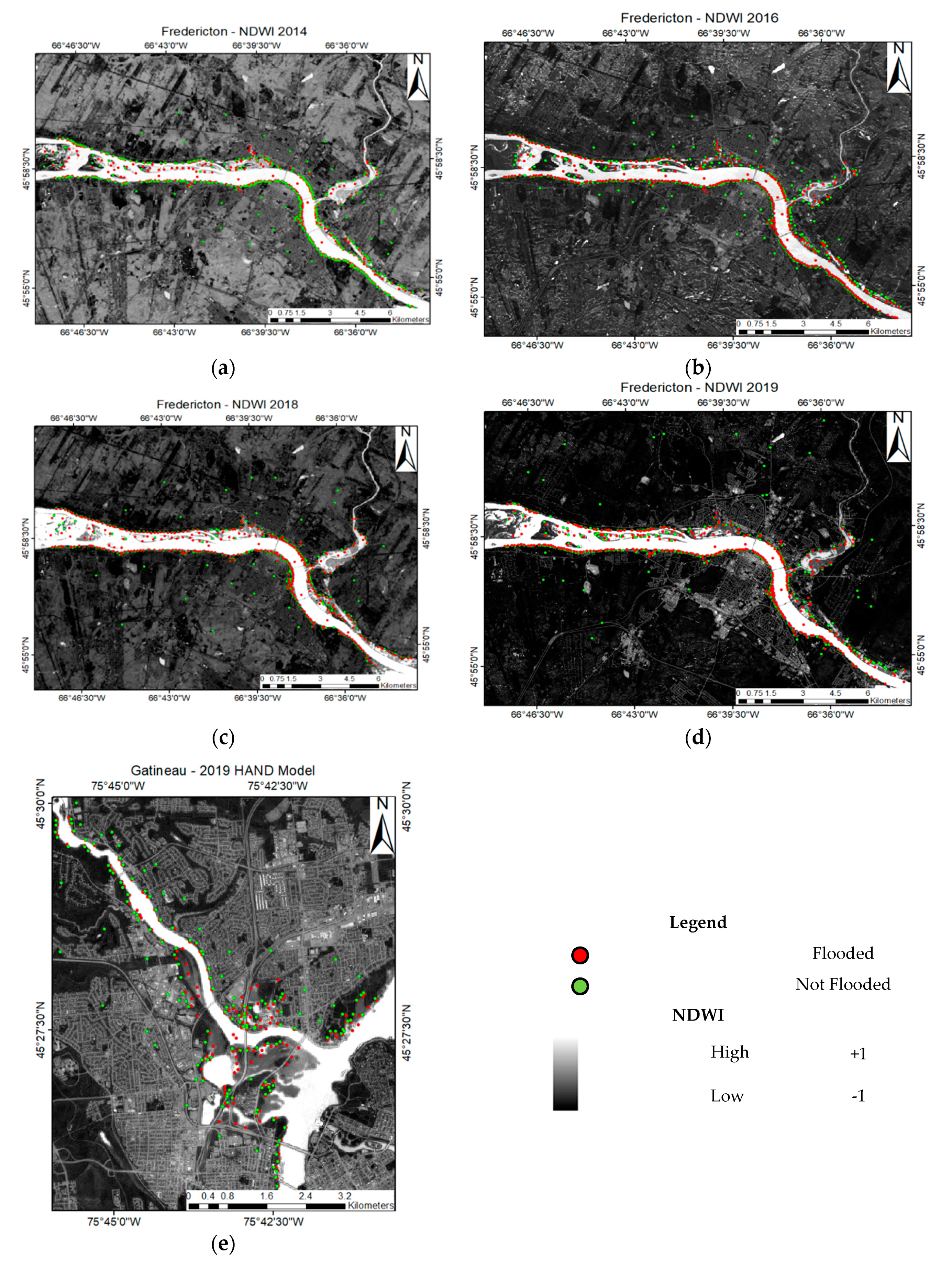
For each flood event, we selected a number of sample points whose label is set to either flooded or not-flooded. We named the points depending on the source of labeling. When we labeled the points as flooded/not flooded using satellite images, we call the points ground truth points. Satellite images capture one instance of floods and clearly show the flooded pixels. Therefore, these labels are considered as ground truth. For the Fredericton and Gatineau study areas, 700 (350 flooded and 350 not flooded) and 330 (165 flooded; 165 not flooded) ground truth points were collected from satellite images, respectively. The points were well-distributed and spread along the floodplains as shown in Figure 3. The ground truth points are only used for accuracy assessment in this study. On the other hand, we labeled the same points using a thresholded HAND model. We call these points pseudo ground truth points. Among the pseudo ground truth points, we selected 10% of them as pseudo training points and 90% of them as validation points.
For accuracy assessment, the ground truth points were selected using a newly developed Normalized Water Difference Index (NDWI) [54] produced from the satellite images (Figure 3). Prior to NDWI calculation, top of the atmosphere correction (TOA) is applied to the images to remove the atmospheric effects from the reflectance values. TOA is applied in QGIS software using the Semi-Automatic Classification Plugin [55]. Equation (1) demonstrates how NDWI is calculated using blue (Blue) and short-wave infrared (SWIR) bands (bands 2 and 6 for Landsat 8 OLI and bands 2 and 11 for Sentinel-2 satellites, respectively). Flooded and not-flooded ground truth points extracted from the NDWIs were mainly selected within the floodplain to assess the capability of the HAND model and PS-RF in generating accurate flood maps.
N D W I = ( B l u e S W I R ) ( B l u e + S W I R ) .
Light Detection and Ranging (LiDAR) data were used to generate the HAND model and three other conditioning factors including Altitude, Slope and Aspect. For the Fredericton datasets, the LiDAR data were obtained from the geographic data catalog website of the Province of New Brunswick (GeoNB) [56]. The LiDAR data were collected in a period of nearly two months, starting on August 2nd, 2015 and continuing to September 28th, 2015, with an average point density of 6 points per square meter. The LiDAR data has a horizontal positional accuracy of ~0.257 m and vertical positional accuracy of 0.275 m which were tested using 216 GPS RTK Survey points [57]. Using available high-resolution LiDAR data, a Digital Terrain Model (DTM) with 1-m resolution was generated for Fredericton area. For the Gatineau dataset, a bare earth High Resolution Digital Elevation Model (HRDEM) [58] was downloaded from the government of Canada website with 1-m resolution. HRDM is a national product of high resolution DTM generated from LiDAR across Canada. The downloaded HRDEM was used to generate the HAND model and Altitude, Slope and Aspect conditioning factors for Gatineau city as was done in the Fredericton study area.

2.3. Conditioning Factors

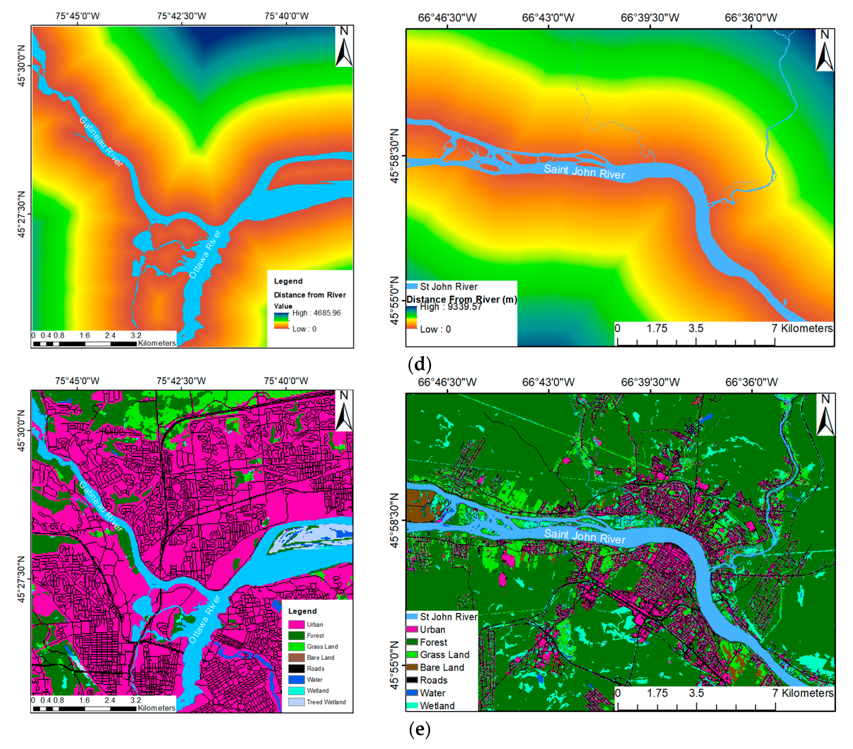
In flood mapping using machine learning, it is crucial to use the appropriate conditioning factors [59]. In a previous case study [44] the best conditioning factors for flood mapping in the Fredericton area were identified. In the study, the effectiveness of 12 different conditioning factors including Altitude, Slope, Aspect, Distance from River, Land use/cover, Terrain Wetness Index (TWI), Terrain Roughness Index (TRI), Stream Power Index (SPI), Curvature, Plan Curvature, Profile Curvature and HAND model were investigated. To find the best combination of conditioning factors, different combinations of the 12 layers were tested as input features of a R.F. classifier. The results confirmed that the combination of five layers, namely Altitude, Slope, Aspect, Distance from River and Land use/cover, provided the highest accuracy. It was found that the Altitude layer is one of the most important conditioning factors for flood mapping [44]. The results also demonstrated that using correlated conditioning factors reduces the accuracy of the R.F. model and a higher number of conditioning factors does not necessarily improve the predictions [44,60]. Thus, for this research, the 5 best conditioning factors namely Altitude, Slope, Aspect, Distance from River and Land use/cover (Figure 4) are used to help with the training of the R.F. model.
For the Fredericton dataset, the Altitude layer, with 1-m spatial resolution, was generated from LiDAR data. Slope and Aspect conditioning factors were derived from the Altitude layer in ArcGIS Desktop 10.6.1 using the Spatial Analyst tool. Distance from River was generated using the Euclidean distance tool within the ArcGIS software and generated from the river boundary shapefile which was obtained from the GeoNB website. The Land use/cover layer was generated by overlaying available polygon shapefiles provided on the GeoNB website. The polygons provided seven classes of Urban, Forest, Grass Land, Bare Land, Roads, Water, Wetlands and were obtained through aerial photography.
The generated conditioning factors for the Gatineau city were derived from HRDEM obtained from the federal governmental website. Conditioning factors were generated using the same tools mentioned earlier within ArcGIS software. The land use/cover layer for the Gatineau dataset was downloaded from Agriculture and Agrifood Canada [61].
Previously mentioned conditioning factors, Altitude, Slope, Aspect and Distance from River had ordinal values that were normalized from 0 to 1 for better consistency in R.F. [62]. All the conditioning factors were covering the same area extent constructing grids of size 1 m2, which resulted in raster sizes of 22,448 columns and 11,533 rows (~258 square kilometers) for the Fredericton region. The same conditions for the Gatineau city were applied and the grids in the Gatineau raster files contained 10,000 columns and 10,000 rows (~100 square kilometers).

2.4. HAND Model

The HAND model is used for several applications such as flood hazard mapping [29], [63], landform classification [17] and remote sensing [64]. As shown in Figure 5, the HAND model is generated through a series of steps. One of the most important requirements of having an accurate HAND model is to use a hydrologically conditioned DTM [17]. To have a proper hydrologically conditioned DTM, a total of 34 culverts and bridges were identified through aerial imagery and OpenStreetMap and burnt using Zonal Statistics Tool and Raster Calculator within ArcMap (Step–1 in Figure 5). Then, the pit holes and depressions in the area were filled using Pit Remove function from the Terrain Analysis Using Digital Elevation Models (TauDEM) suite within ArcGIS [65] (Step–2 in Figure 5). By burning culverts and bridges and filling depressions we ensured that our DTM does not contain erroneous flow directions. Then, the flow direction raster was computed using D-Infinity Flow Directions function from TauDEM, in which the flow is calculated through a triangular facet [66] (Step–3 in Figure 5). The last required component of the HAND model is the stream raster which will be considered as the elevation reference of the model and elevation of all pixels will be calculated from this layer, hence, it is necessary to ensure that the stream raster is accurate. The stream raster can be obtained through D-8 Flow Direction and thresholding the major stream based on Strahler stream order [29,67] but, since the stream shapefiles representing all the streams of the province were available in the GeoNB and Ottawa Open Data [68], geospatial databases for Fredericton and Gatineau respectively, we rasterized the shapefile and used it as our stream raster. D-Infinity Distance Down function available in TauDEM software is the last step which generates the HAND model. Different distance and statistical methods of calculation are available within this tool but for the HAND model generation Vertical method for Distance and Average for Statistical are selected (Step–4 in Figure 5). Once the HAND model is generated through the steps, the model can be used to demonstrate inundated areas based on the water level rise. To do that, the water level difference should be calculated based on the observations from gauge station and the HAND model. For more details on the HAND model, readers can refer to References [17,69].
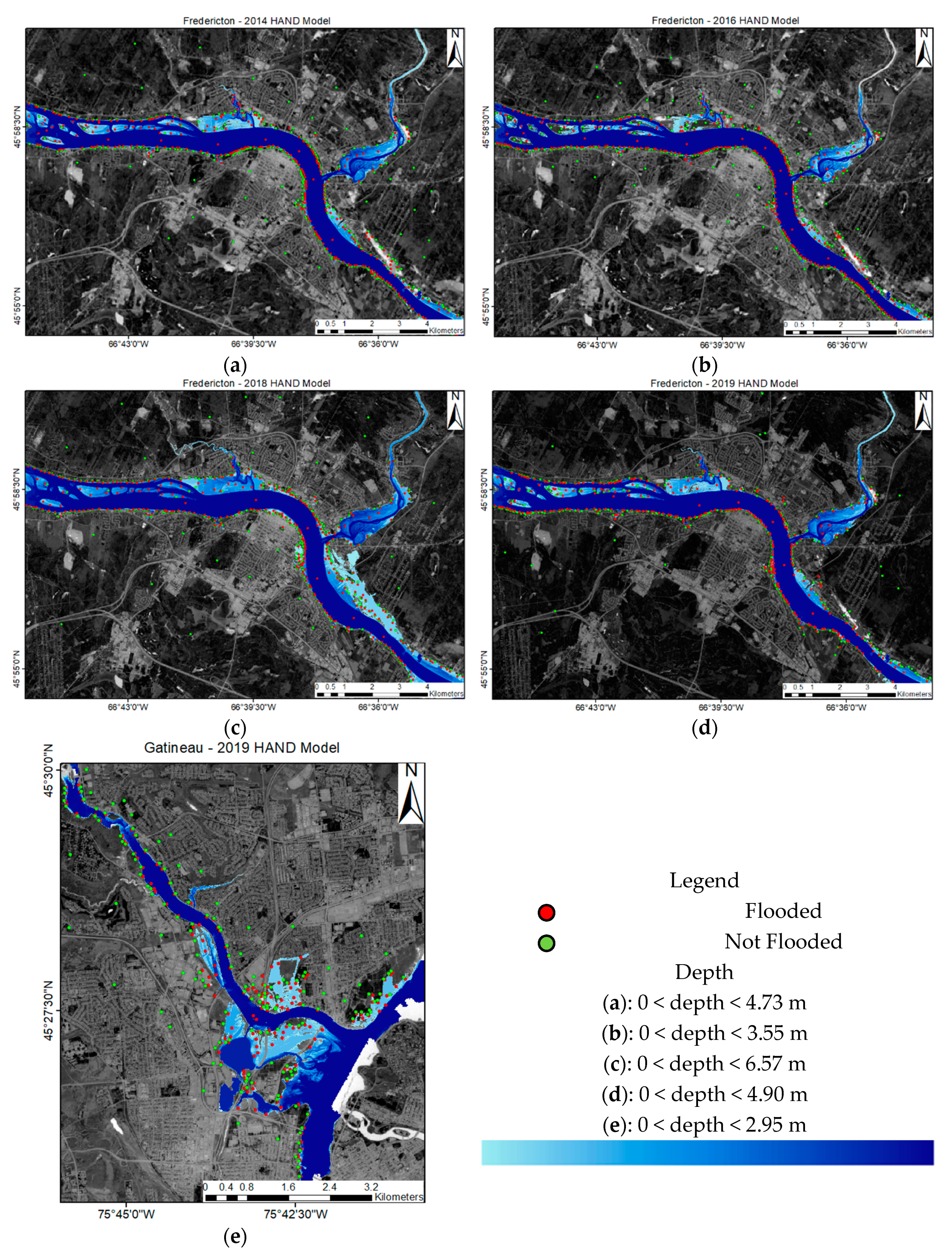
To generate an early estimation of the flood extent, the HAND model is thresholded based on the water level as recorded by the local river gauge. To properly threshold the HAND model, the difference of water level at the time of flood and at the time of LiDAR data collection should be calculated and the model should be thresholded based on that difference [30]. As previously mentioned, in the Fredericton dataset, the LiDAR data were collected in a period of approximately two months from August 2nd, 2015 continuing to September 28th, 2015 and during that time the river water level fluctuated from 1.121 m to 1.854 m. We have used the average water level over that period as the river water level at the time of LiDAR data collection which is equal to 1.46 m. So, the threshold for all the Fredericton datasets were calculated by subtracting the average 1.46 m from the water level at the time of the flood event. The reference water level for the Ottawa River was considered to be 42.04 m which was obtained through gauge readings at the time of data collection. Figure 6 shows the HAND models generated for the five flood events discussed in this study.

2.5. Random Forest

R.F. is a supervised machine learning model and one of the most robust classifiers that makes decisions based on the average of the results of a multitude of decision trees [70]. The classifier fits an arbitrary number of trees on different features of the datasets and by averaging multiple predictions controls the over-fitting issue. R.F. was selected because of its capability to handle noisy data, its efficiency to take features with different natures and its ability to rank the features based on their degree of importance [70,71]. The feature with the highest degree of importance is the major splitter in all the trees.

2.6. Pseudo Supervised Random Forest (PS-RF)

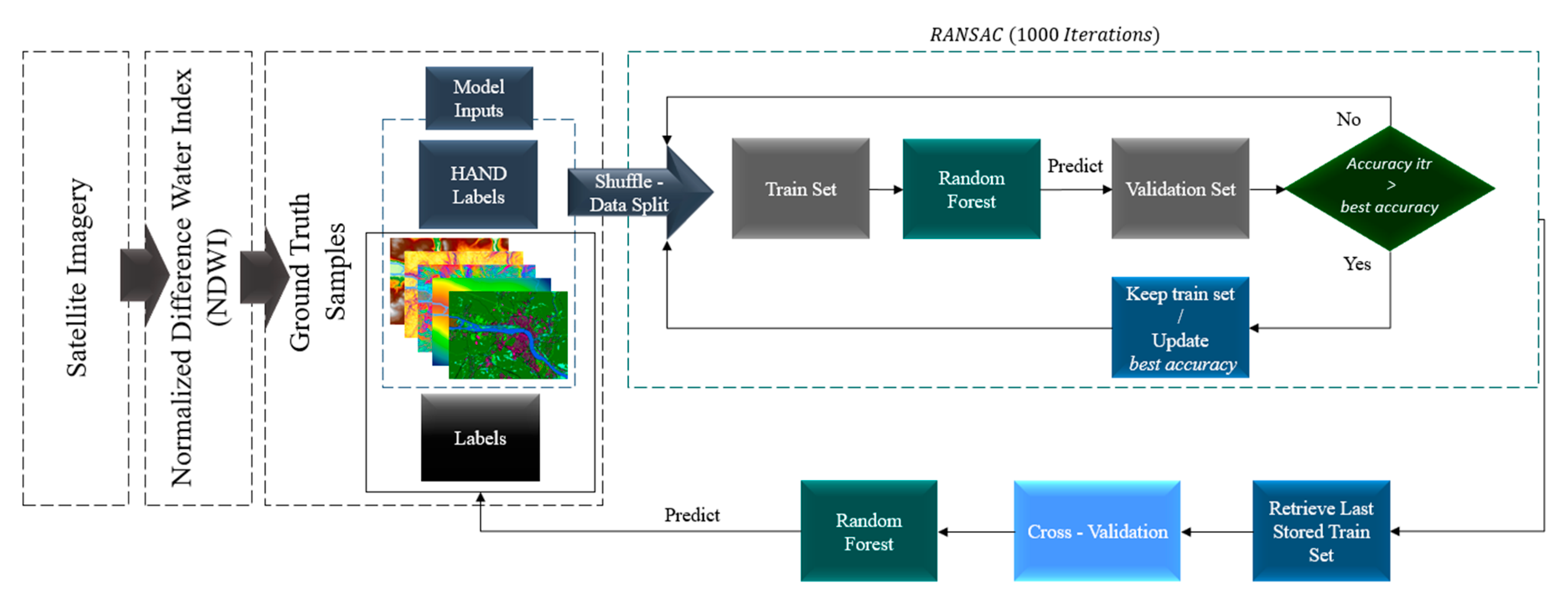
Figure 7 demonstrates the workflow of the proposed PS-RF model. In PS-RF, we used the HAND model predictions as pseudo labels to train a R.F. classifier in Python within Scikit-Learn library [72]. However, due to the deficiencies of the HAND model discussed previously, the pseudo labels obtained from the HAND model are not 100% accurate. Therefore, we need to detect the outliers and remove them so that the R.F. algorithm is trained with the most reliable pseudo training points. For selecting the best pseudo training points and removing the outliers, the RANSAC paradigm was used. Through the RANSAC process, the HAND model is used as a cost function for R.F. optimization. Through iterations and training R.F. by randomly selected pseudo training points, the best training subset is selected and as it is evident from Figure 8, different training subsets achieve various accuracies. So, the outliers involved in training data provided by the HAND model will be identified.
First, the dataset, including 700 pseudo ground truth points for Fredericton and 330 pseudo ground truth points for Gatineau, with values from conditioning factors and pseudo labels (flooded and not-flooded labels from the HAND model) are randomly split into two subsets of 10% training (in fact pseudo training) and 90% validation. The R.F. algorithm is then trained by the pseudo training data and used to predict the validation subset. The overall accuracy of the validation subset is checked against the HAND model. This accuracy number is stored and the process is repeated 1000 times to make sure different combinations of pseudo training points from the dataset are used to train R.F. Over the iteration process, the pseudo training subset is updated each time the process reaches a higher accuracy than previous predictions over the validation subset.
Once 1000 iterations were completed, the best pseudo training subset was used to train the R.F. model. Also, the model hyperparameters including the number of trees (n_estimators), the minimum number of samples (min_sample_split), minimum number of samples at a leaf (min_samples_leaf) and maximum depth of trees (max_depth) are optimized through 5-fold Cross-Validation. Then, the R.F. model which was trained by the best-achieved pseudo training subset is used to predict the ground truth points of the whole dataset.

3. Results

In this study, different measures for accuracy assessment were applied to compare the performance of our results from PS-RF to that of a thresholded HAND model. To assess the accuracy of PS-RF we used accuracy measures such as true positive rate (TPR), true negative rate (TNR), false positive rate (FPR), false negative rate (FNR), overall accuracy, Cohen’s Kappa Coefficient [73] and Matthews Correlation Coefficient (MCC) [74] which are depicted in Table 2.
TPR (Sensitivity) and TNR (Specificity) indices show the probability of correctly predicted flooded and not-flooded points by the HAND model and the proposed model. FPR and FNR indices show the percentage of flooded and not-flooded points which were misclassified. Cohen’s Kappa Coefficient represents the rate of likeliness between ground truth and predicted data and its values are interpreted as: None 0–0.20, Minimal 0.21–0.39, Weak 0.40–0.59, Moderate 0.60–0.79, Strong 0.80–0.90 and Almost Perfect likeliness for values of above 0.90 [75]. Due to recent concerns about Cohen’s Kappa Coefficient assessments and its undesired behavior discussed in Reference [76], the MCC metric was also calculated to ensure the validity of our evaluation. MCC values close to 1 represent perfect agreement, the value of 0 is interpreted as random prediction and the value of −1 is interpreted as complete opposite predictions for observations. Calculated indices are all based on four parameters of true positive (T.P.), true negative (T.N.), false positive (F.P.) and false negative (F.N.). In Cohen’s Kappa Coefficient, P 0 and P e are relative observed agreement and the hypothetical probability of chance agreement, respectively.
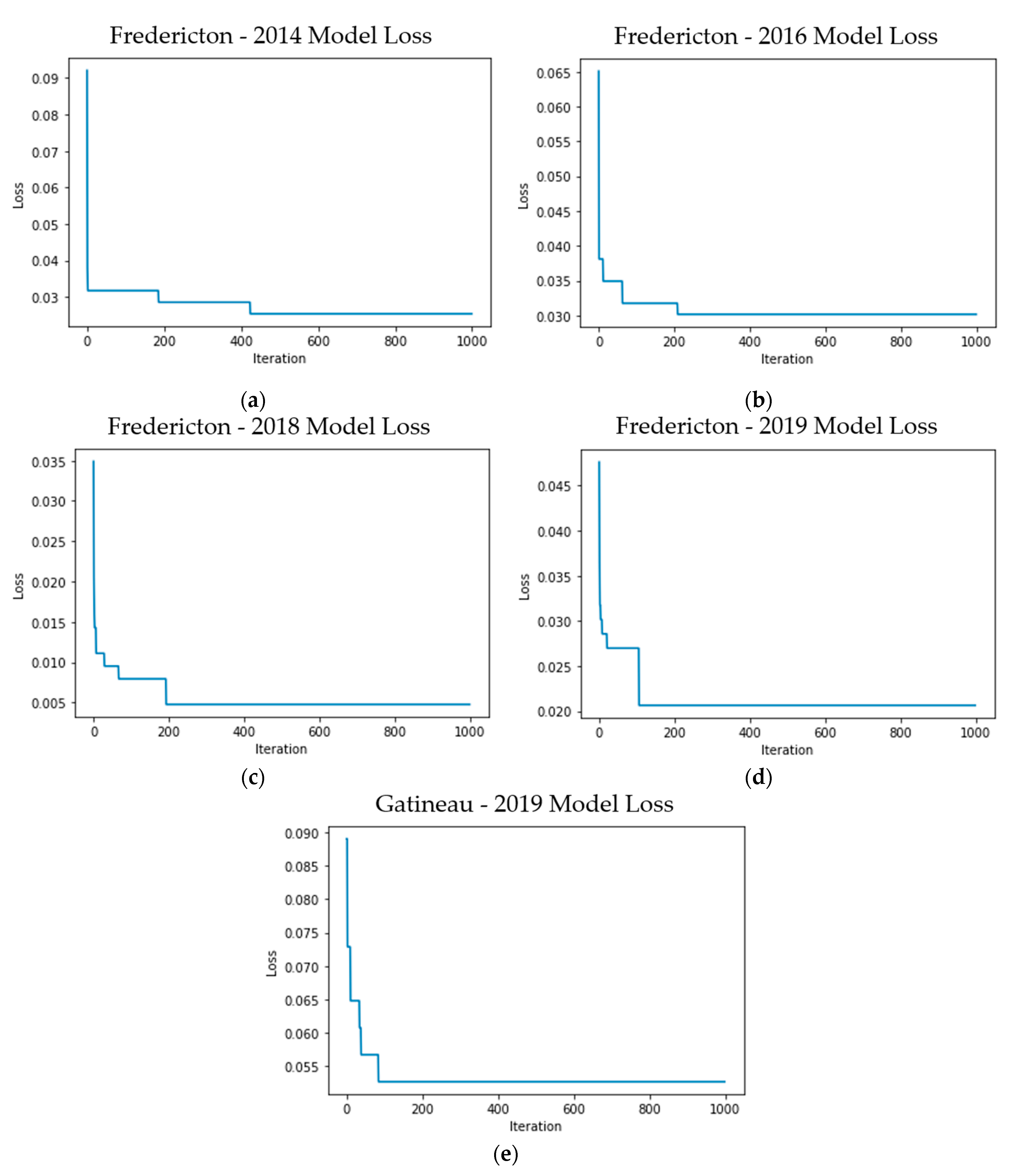
Figure 8 represents the Model Loss for the five periods. The vertical axis of the figures demonstrates how the prediction accuracy over validation data has improved and higher accuracy was obtained by selecting diverse subsets of pseudo ground truth points provided by the HAND model. The horizontal axis is the implemented iteration number. In the 2014 dataset, the R.F. model accuracy over validation data were improved by 0.06 through the iteration process. In 2016, it can be seen that an improvement of nearly 0.04 was achieved through iteration. In 2018, the accuracy for R.F. model was enhanced by 0.03 over validation data through shuffling and selecting training data randomly among our pseudo ground truth points. R.F. predictions for 2019 were also enhanced over validation data by 0.025 through randomly selecting pseudo training data. In the Gatineau flood event that occurred in 2019, there was an improvement of around 0.04 through the iteration process.
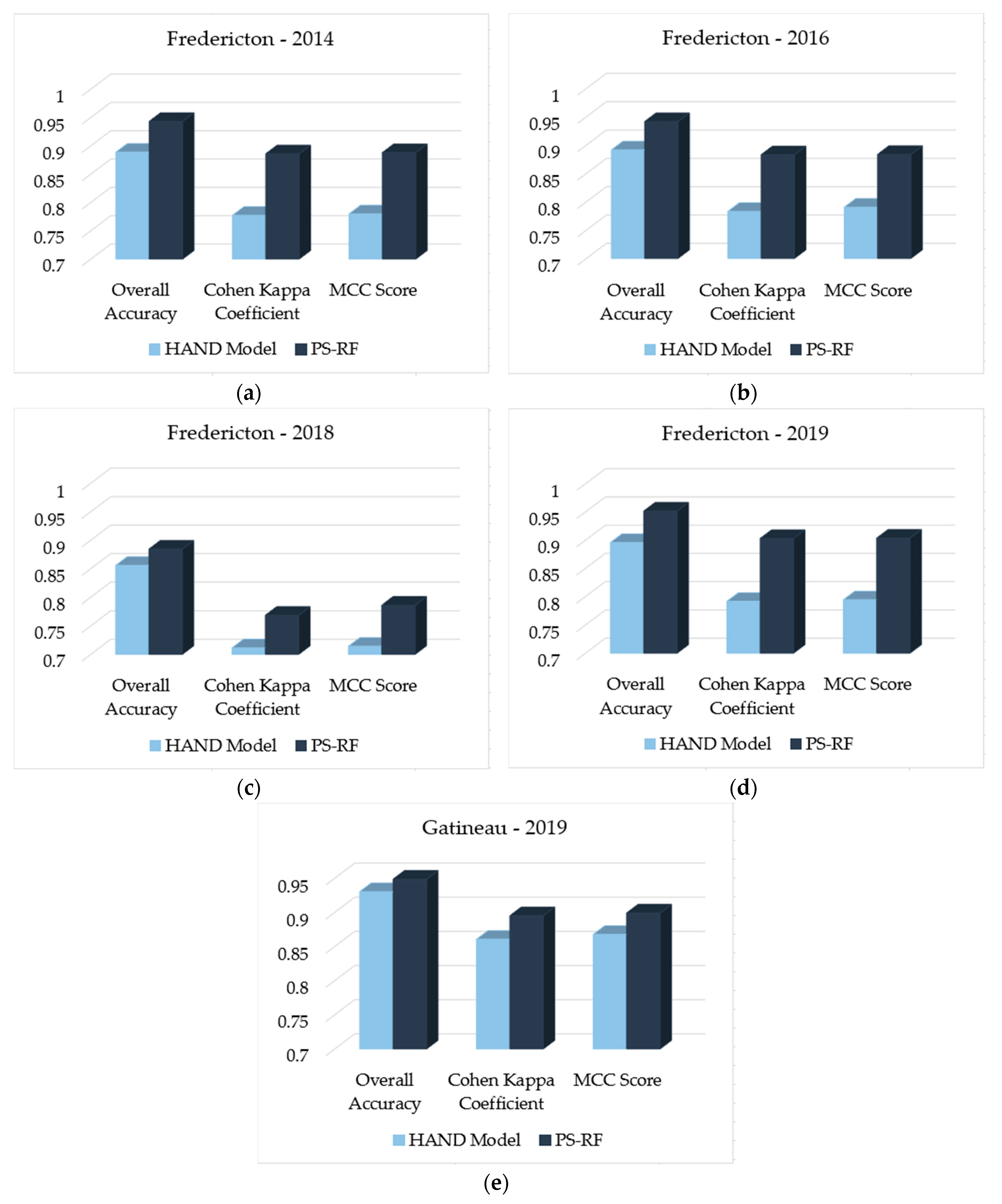
The achieved overall accuracy, which represents the closeness of predictions to their true classes, shows that PS-RF has improved the accuracy of the HAND model in all the five flood events (Figure 9). In the 2014 Fredericton flood event, PS-RF reached an overall accuracy of 94.23% compared to 88.86% from the HAND model. Also, PS-RF was ~11% higher than HAND in both Cohen’s and MCC respectively. In the 2016 Fredericton flood event, the PS-RF model has improved the accuracy of the HAND model by 5% with 94.14% accuracy for PS-RF and 89.14% accuracy for the HAND model. Cohen’s and MCC metrics were 10% and ~9.5% higher for PS-RF than HAND in 2016 as well. 2018 flood event predictions were nearly similar but still, PS-RF obtained a higher accuracy with 88.43% overall accuracy for PS-RF and 85.57% for the HAND model. In 2018, PS-RF had Cohen’s of ~77% which is ~6% higher than HAND and MCC score of ~79% which is ~7% higher than HAND. In the 2019 Fredericton flood event, PS-RF was able to reach an overall accuracy of ~95% compared to ~90% for the HAND model with ~11% higher Cohen’s and MCC score. In Gatineau 2019 flood event, the overall accuracy of PS-RF was 94.85% while the HAND model reached 93.03%. PS-RF’s Cohen’s and MCC score for Gatineau 2019 flood event were ~3.5% and ~3% higher than HAND, respectively.
The Cohen’s and MCC results show that PS-RF has outperformed the HAND model in all the five years of interest and the degree of likeliness in the prediction of flooded and not-flooded points is superior to HAND model according to Cohen’s Kappa Coefficient values. Also, higher values of the MCC index obtained by PS-RF show better classification quality than the HAND model. TPR, FPR, TNR and FNR indices are discussed next and demonstrated in Figure 10 for the HAND model and PS-RF.
To analyze the HAND model and PS-RF accuracy in detecting flood extent, TPR, FPR, TNR and FNR indices were calculated. The accuracy indexes are presented in Figure 10 and discussed further in the discussion section.

4. Discussion

PS-RF was tested in 5 different flood events and resulted in higher accuracy than the HAND model in all. In flood mapping, it is very important to provide precise estimations and the model should not over or underestimate the flood extent. To analyze the performance the HAND model in estimating the extent of 5 tested flood events, different accuracy metrics were calculated and are discussed below.
The Fredericton 2014 flood event, the HAND model has correctly predicted ~85% of flooded ground truth points while PS-RF achieved ~98%. In the case of not-flooded points, the HAND model performed slightly better with TNR value of ~93% compared to ~91% for PS-RF. This means PS-RF was able to perform better in detecting flooded points but the HAND model had a better performance in detecting not-flooded points (Figure 10a). In the Fredericton 2016 flood event, PS-RF performed better in predicting both flooded and not-flooded points with ~9% and ~1% higher TPR and TNR values (Figure 10b), respectively. The Fredericton 2018 flood event contained nearly similar results for PS-RF and HAND model with PS-RF achieving ~9% higher TPR and ~3% lower TNR compared to the HAND model (Figure 10c). In the Fredericton 2019 flood event, PS-RF obtained ~11% higher TPR and ~0.3% lower TNR (Figure 10d). In the Fredericton 2016, 2018 and 2019 floods, PS-RF performed better in detecting both flooded and not-flooded ground truth points than the HAND model. However, in the Gatineau 2019 flood event, PS-RF was able to reach a TPR value of ~93% compared to ~87% from the HAND model. However, the HAND model performed better in detecting not-flooded points with ~2% higher TNR value (Figure 10e). The HAND model can estimate the inundated areas given the depth of water. Therefore, it can produce a dynamic flood mapping model. However, since it is a simplified model, it suffers from having a limited accuracy as reported in different studies [30]. In this study, we proposed a new model that achieved better results compared to a HAND model. We trained an R.F. model to benefit from different conditioning factors, that is, altitude, slope, aspect, distance from river and land use/cover, to adjust the flood borders produced by the HAND model. Thus, this model combines the HAND results with different conditioning factors to improve the accuracy of the final flood maps.
In PS-RF, the predictions of the HAND model are used as the presumptive labels of ground truth points to train R.F. model with five conditioning factors of Altitude, Slope, Aspect, Distance from River and Land use/cover. However, as concluded previously, the HAND model estimations contain errors that need to be eliminated from the pseudo training subset. To remove the HAND model errors, the RANSAC paradigm was employed. The philosophy of RANSAC is to use as little data as possible to train a model while attempting to remove the errors [46]. Thus, to find the optimum percentage of the pseudo training points, different percentage numbers including 10%, 15%, 25%, 50%, 70% and 90% were tested over the 2016 Fredericton and 2019 Gatineau datasets. These pseudo training points are used to train the R.F. model. Figure 11 demonstrates the overall accuracy of the R.F. with different training percentages over the test subset. For comparison only, we displayed the HAND model accuracy in the figure as well.
Since the datasets for Fredericton flood events include the same number of ground truth points, different pseudo training subsets were tested over Fredericton 2016 flood event. As is evident in Figure 11a, the highest overall accuracy, 92.86%, was obtained using 10% pseudo training points and as the training subset was increased, the overall accuracy has become more similar to that of the HAND model. In the Fredericton dataset, where the pseudo training subset was 70%, an overall accuracy of 91.29% was obtained and where it was 90% an overall accuracy of 91.14% was obtained which is similar to the HAND model overall accuracy. In the Gatineau dataset, the highest overall accuracy, 93.94%, was obtained by 15% training data. By increasing the pseudo training percentage to 25%, the overall accuracy reaches 93.48% which is slightly higher than the HAND with 93.03% overall accuracy. As shown in Figure 11b, other training amounts achieved overall accuracies fairly similar to that of the HAND model while the 15% one attained the highest rate. The results of this study showed how the HAND model can provide pseudo training data for R.F. to model flood events. Through this integration, the required training data for R.F. was obtained and the flood events were modeled with a higher accuracy than by the HAND model.
In this study, we proposed to improve the performance of the HAND model in flood mapping by integrating it with one of the most robust machine learning models, R.F. The R.F. model is used in different studies including [19,35] for generating flood susceptibility maps by using the geospatial information of abundant available inundated locations as training data. In these studies, the R.F. model makes predictions based on the data related to previous flood events; therefore, the model provides a general assessment of areas that are at risk of flooding by using datasets from multiple flood events. However, the required training data for R.F. might not be always available for all the locations, which makes the use of R.F. very strict in this context. Hence, we proposed to use a simplified conceptual model to provide the training data for R.F. to dynamically identify the inundated areas.

5. Conclusions

Near-real time flood mapping requires efficient and accurate estimations. Previous techniques for flood mapping either lack the necessary precision or are very costly and intricate for rapid implementation. In this research, a new model, named PS-RF, was developed for flood mapping through the integration of a simplified conceptual model, HAND and a robust machine learning model, R.F. This model was tested on 5 different flood events occurred in Fredericton and Gatineau achieving higher overall accuracy in all the events compared to the HAND model. First, the HAND model was used to simulate the extent of the flood events based on the river water level. To improve the accuracy of flood maps obtained from the HAND model, the RANSAC methodology was used to filter out the outliers from pseudo ground truth points and maintain the most established ones. Then, those most certain pseudo ground truth points were used as pseudo training points for R.F. model. Next, the trained R.F. model was used to estimate the overall flood extent in the area. The proposed model obtained higher accuracy than the HAND model in all five years of interest. Also, by integrating the HAND model and R.F., the required training data for the R.F. model were provided through the HAND. This approach can be implemented in areas with different climate and topography where a high resolution DTM is available; however, varied conditioning factors might be selected for other regions depending on the characteristics of a region. In our future work, we will consider how the feature selection can be further automated using different optimization algorithms which will result in a more complete flood mapping procedure.

Author Contributions

M.E. implemented the experiments and wrote the paper; G.A. implemented the experiments; S.J. analyzed the results and reviewed this paper; H.M. helped to provide data and reviewed this paper; D.C. reviewed this paper. All authors have read and agreed to the published version of the manuscript.

Funding

The authors would like to thank New Brunswick Innovation Foundation (NBIF), grant number RAI2019-026” and “Natural Sciences and Engineering Research Council of Canada (NSERC), grant number RGPIN 170227-2013” for funding this research.

Acknowledgments

The authors would like to thank GeoNB, Ottawa Open Data, Landsat, Senintel-2, Natural Resource Canada (NRCAN) and Terrain Analysis Using Digital Elevation Models (TauDEM) suite providers.

Conflicts of Interest

The authors declare no conflict of interest.

References

  1. Tehrany, M.S.; Lee, M.-J.; Pradhan, B.; Jebur, M.N.; Lee, S. Flood susceptibility mapping using integrated bivariate and multivariate statistical models. Environ. Earth Sci. 2014, 72, 4001–4015. [Google Scholar] [CrossRef]
  2. Thistlethwaite, J.; Henstra, D.; Brown, C.; Scott, D. How flood experience and risk perception influences protective actions and behaviours among Canadian homeowners. Environ. Manag. 2018, 61, 197–208. [Google Scholar] [CrossRef]
  3. Messner, F.; Meyer, V. Flood damage, vulnerability and risk perception–challenges for flood damage research. In Flood Risk Management: Hazards, Vulnerability and Mitigation Measures; Springer: Berlin/Heidelberg Germany, 2006; pp. 149–167. [Google Scholar]
  4. Ghoneim, E.; Foody, G.M. Assessing flash flood hazard in an arid mountainous region. Arab. J. Geosci. 2013, 6, 1191–1202. [Google Scholar] [CrossRef]
  5. Nicholls, R.; Burcharth, H.F.; Zanuttigh, B.; Andersen, T.L.; Orcid, L.; Lara, J.L.; Steendam, G.j.; Roul, P.; Sergent, P.; Ostrowski, R.; et al. Developing a holistic approach to assessing and managing coastal flood risk. In Coastal Risk Management in a Changing Climate; Elsevier—Butterworth-Heinemann: Oxford, UK, 2015; pp. 9–53. [Google Scholar]
  6. Gaur, A.; Gaur, A.; Simonovic, S.P. Future Changes in Flood Hazards across Canada under a Changing Climate. Water 2018, 10, 1441. [Google Scholar] [CrossRef] [Green Version]
  7. Schiermeier, Q. Increased flood risk linked to global warming: Likelihood of extreme rainfall may have been doubled by rising greenhouse-gas levels. Nature 2011, 470, 316–317. [Google Scholar] [CrossRef] [PubMed] [Green Version]
  8. Brunner. HEC-RES River Analysis System—User’s Manual Version 5.0. US Army Corps of Engineers; Institute for Water Resources, Hydrologic Engineering Center (HEC): Davis, CA, USA, 2016; p. 962. [Google Scholar]
  9. DHI. MIKE 11—A Modelling System for Rivers and Channels—User Guide; DHI: Hørsholm, Denmark, 2003; p. 430. [Google Scholar]
  10. DHI. MIKE 21-2D Modelling of Coast and Sea; DHI Water & Environment Pty Ltd.: Hørsholm, Denmark, 2012. [Google Scholar]
  11. Moulinec, C.; Denis, C.; Pham, C.-T.; Rougé, D.; Razafindrakoto, J.-M.; Razafindrakoto, E.; Barber, R.W.; Emerson, D.R.; Gu, X.-J. TELEMAC: An efficient hydrodynamics suite for massively parallel architectures. Comput. Fluids 2011, 51, 30–34. [Google Scholar] [CrossRef] [Green Version]
  12. Prakash, M.; Rothauge, K.; Cleary, P.W. Modelling the impact of dam failure scenarios on flood inundation using SPH. Appl. Math. Model. 2014, 38, 5515–5534. [Google Scholar] [CrossRef]
  13. Vacondio, R.; Rogers, B.D.; Stansby, P.K.; Mignosa, P. SPH modeling of shallow flow with open boundaries for practical flood simulation. J. Hydraul. Eng. 2012, 138, 530–541. [Google Scholar] [CrossRef]
  14. Smith, L.C. Satellite remote sensing of river inundation area, stage, and discharge: A review. Hydrol. Process. 1997, 11, 1427–1439. [Google Scholar] [CrossRef]
  15. Schumann, G.; Bates, D.P.; Horritt, S.M.; Matgen, P.; Pappenberger, F. Progress in integration of remote sensing-derived flood extent and stage data and hydraulic models. Rev. Geophys. 2009, 47. [Google Scholar] [CrossRef]
  16. Lhomme, J.; Sayers, P.; Gouldby, B.; Samuels, P.; Wills, M.; Mulet-Marti, J. Recent development and application of a rapid flood spreading method. In Proceedings of the FLOODrisk, Keble College, Oxford, UK, 30 September–2 October 2008. [Google Scholar]
  17. Nobre, A.D.; Nobre, A.D.; Cuartas, L.A.; Hodnett, M.; Rennó, C.D.; Rodrigues, G.; Silveira, A.; Saleska, S. Height Above the Nearest Drainage—A hydrologically relevant new terrain model. J. Hydrol. 2011, 404, 13–29. [Google Scholar] [CrossRef] [Green Version]
  18. Tehrany, M.S.; Pradhan, B.; Jebur, M.N. Flood susceptibility mapping using a novel ensemble weights-of-evidence and support vector machine models in GIS. J. Hydrol. 2014, 512, 332–343. [Google Scholar] [CrossRef]
  19. Rahmati, O.; Pourghasemi, H.R.; Melesse, A.M. Application of GIS-based data driven random forest and maximum entropy models for groundwater potential mapping: A case study at Mehran Region, Iran. Catena 2016, 137, 360–372. [Google Scholar] [CrossRef]
  20. Zhao, G.; Pang, B.; Xu, Z.; Peng, D.; Xu, L. Assessment of urban flood susceptibility using semi-supervised machine learning model. Sci. Total Environ. 2019, 659, 940–949. [Google Scholar] [CrossRef] [PubMed]
  21. Pourghasemi, H.R.; Kariminejad, N.; Amiri, M.; Edalat, M.; Zarafshar, M.; Blaschke, T.; Cerda, A. Assessing and Mapping Multi-Hazard Risk Susceptibility Using a Machine Learning Technique|Scientific Reports. 2020. Available online: https://www.nature.com/articles/s41598-020-60191-3 (accessed on 30 April 2020).
  22. Teng, J.; Jakeman, A.J.; Vaze, J.; Croke, B.F.; Dutta, D.; Kim, S. Flood inundation modelling: A review of methods, recent advances and uncertainty analysis. Environ. Model. Softw. 2017, 90, 201–216. [Google Scholar] [CrossRef]
  23. Brunner, G.W.; Piper, S.S.; Jensen, M.R.; Chacon, B. Combined 1D and 2D hydraulic modeling within HEC-RAS. In World Environmental and Water Resources Congress; ASCE: Austin, TX, USA, 2015; pp. 1432–1443. [Google Scholar]
  24. Monaghan, J.J. Simulating free surface flows with SPH. J. Comput. Phys. 1994, 110, 399–406. [Google Scholar] [CrossRef]
  25. Ye, J.; McCorquodale, J.A. Simulation of curved open channel flows by 3D hydrodynamic model. J. Hydraul. Eng. 1998, 124, 687–698. [Google Scholar] [CrossRef]
  26. Sidrane, C.; Fitzpatrick, D.J.; Annex, A.; O’Donoghue, D.; Gal, Y.; Biliński, P. Machine Learning for Generalizable Prediction of Flood Susceptibility. arXiv 2019, arXiv:1910.06521. [Google Scholar]
  27. Rennó, C.D.; Nobre, A.D.; Cuartas, L.A.; Soares, J.V.; Hodnett, M.G.; Tomasella, J. HAND, a new terrain descriptor using SRTM-DEM: Mapping terra-firme rainforest environments in Amazonia. Remote Sens. Environ. 2008, 112, 3469–3481. [Google Scholar] [CrossRef]
  28. Momo, M.R. Evaluation of the Application of the HAND model in Mapping of Areas Susceptible to Flooding in the Municipality of Blumenau. Ph.D. Thesis, Tese de Mestrado em Engenharia Ambiental, Fundação Universidade Regional de, Blumenau, Brazil, 2014. (In Spanish). [Google Scholar]
  29. McGrath, H.; Bourgon, J.-F.; Proulx-Bourque, J.-S.; Nastev, M.; el Ezz, A.A. A comparison of simplified conceptual models for rapid web-based flood inundation mapping. Nat. Hazards 2018, 93, 905–920. [Google Scholar] [CrossRef]
  30. Nobre, A.D.; Cuartas, L.A.; Momo, M.R.; Severo, D.L.; Pinheiro, A.; Nobre, C.A. HAND contour: A new proxy predictor of inundation extent. Hydrol. Process. 2016, 30, 320–333. [Google Scholar] [CrossRef]
  31. Toth, E.; Brath, A.; Montanari, A. Comparison of short-term rainfall prediction models for real-time flood forecasting. J. Hydrol. 2000, 239, 132–147. [Google Scholar] [CrossRef]
  32. Falah, F.; Rahmati, O.; Rostami, M.; Ahmadisharaf, E.; Daliakopoulos, I.N.; Pourghasemi, H.R. Artificial neural networks for flood susceptibility mapping in data-scarce urban areas. In Spatial Modeling in GIS and R for Earth and Environmental Sciences; Elsevier: Amsterdam, The Netherlands, 2019; pp. 323–336. [Google Scholar]
  33. Tehrany, M.S.; Pradhan, B.; Mansor, S.; Ahmad, N. Flood susceptibility assessment using GIS-based support vector machine model with different kernel types. Catena 2015, 125, 91–101. [Google Scholar] [CrossRef]
  34. Tehrany, M.S.; Pradhan, B.; Jebur, M.N. Flood susceptibility analysis and its verification using a novel ensemble support vector machine and frequency ratio method. Stoch. Environ. Res. A Risk Assess. 2015, 29, 1149–1165. [Google Scholar] [CrossRef]
  35. Lee, S.; Kim, J.-C.; Jung, H.-S.; Lee, M.J.; Lee, S. Spatial prediction of flood susceptibility using random-forest and boosted-tree models in Seoul metropolitan city, Korea. Geomat. Nat. Hazards Risk 2017, 8, 1185–1203. [Google Scholar] [CrossRef] [Green Version]
  36. Zhao, G.; Pang, B.; Xu, Z.; Yue, J.; Tu, T. Mapping flood susceptibility in mountainous areas on a national scale in China. Sci. Total Environ. 2018, 615, 1133–1142. [Google Scholar] [CrossRef]
  37. Khu, S.T.; Liong, S.-Y.; Babovic, V.; Madsen, H.; Muttil, N. Genetic programming and its application in real-time runoff forecasting 1. JAWRA J. Am. Water Resour. Assoc. 2001, 37, 439–451. [Google Scholar] [CrossRef]
  38. Rahmati, O.; Pourghasemi, H.R.; Zeinivand, H. Flood susceptibility mapping using frequency ratio and weights-of-evidence models in the Golastan Province, Iran. Geocarto Int. 2016, 31, 42–70. [Google Scholar] [CrossRef]
  39. Khosravi, K.; Nohani, E.; Maroufinia, E.; Pourghasemi, H.R. A GIS-based flood susceptibility assessment and its mapping in Iran: A comparison between frequency ratio and weights-of-evidence bivariate statistical models with multi-criteria decision-making technique. Nat. Hazards 2016, 83, 947–987. [Google Scholar] [CrossRef]
  40. Pradhan, B. Flood susceptible mapping and risk area delineation using logistic regression, GIS and remote sensing. J. Spat. Hydrol. 2010, 9, 1–18. [Google Scholar]
  41. Tehrany, M.S.; Pradhan, B.; Jebur, M.N. Spatial prediction of flood susceptible areas using rule based decision tree (DT) and a novel ensemble bivariate and multivariate statistical models in GIS. J. Hydrol. 2013, 504, 69–79. [Google Scholar] [CrossRef]
  42. Haq, M.; Akhtar, M.; Muhammad, S.; Paras, S.; Rahmatullah, J. Techniques of Remote Sensing and GIS for flood monitoring and damage assessment: A case study of Sindh province, Pakistan. Egypt. J. Remote Sens. Space Sci. 2012, 15, 135–141. [Google Scholar] [CrossRef] [Green Version]
  43. Pradhan, B.; Hagemann, U.; Tehrany, M.S.; Prechtel, N. An easy to use ArcMap based texture analysis program for extraction of flooded areas from TerraSAR-X satellite image. Comput. Geosci. 2014, 63, 34–43. [Google Scholar] [CrossRef]
  44. Esfandiari, M.; Jabari, S.; McGrath, H.; Coleman, D. Flood mapping using Random Forest and Identifying the essential conditioning factors; A case study in Fredericton, New Brunswick, Canada. ISPRS Ann. Photogramm. Remote Sens. Spat. Inf. Sci. 2020, 3, 609–615. [Google Scholar] [CrossRef]
  45. Lee, D.-H. Pseudo-label: The simple and efficient semi-supervised learning method for deep neural networks. In Workshop on Challenges in Representation Learning, ICML; Kaggle: San Francisco, CA, USA, 2013; Volume 3. [Google Scholar]
  46. Fischler, M.a.; Bolles, R.C. Random sample consensus: A paradigm for model fitting with. Commun. ACM 1981, 24, 381–395. [Google Scholar] [CrossRef]
  47. McGrath, H.; Stefanakis, E.; Nastev, M. Rapid risk evaluation (ER 2) using MS excel spreadsheet: A case study of Fredericton (New Brunswick, Canada). ISPRS Ann. Photogramm. Remote Sens. Spat. Inf. Sci. 2016, 3, 27. [Google Scholar] [CrossRef]
  48. Ottawa Riverkeeper’s River Report, Ecology and Impacts. 2006. Available online: https://www.ottawariverkeeper.ca/wp-content/uploads/2018/01/River-Report-English.pdf.pdf (accessed on 10 June 2020).
  49. ET|Last Updated: May 4, and 2019, Under Water, again|CBC News. CBC. 4 May 2019. Available online: https://www.cbc.ca/news/canada/ottawa/ottawa-river-flooding-2019-recap-1.5119980 (accessed on 10 June 2020).
  50. AT|Last Updated: April 30, and 2018, Worst Floods in New Brunswick History: How 2018 Compares|CBC News. CBC. 30 April 2018. Available online: https://www.cbc.ca/news/canada/new-brunswick/st-john-river-flooding-history-1.4641969 (accessed on 7 May 2020).
  51. Fathollahi, F.; Zhang, Y. Adaptive band selection for pan-sharpening of hyperspectral images. Int. J. Remote Sens. 2020, 41, 3924–3947. [Google Scholar] [CrossRef]
  52. Jabari, S.; Fathollahi, F.; Roshan, A.; Zhang, Y. Improving UAV imaging quality by optical sensor fusion: An initial study. Int. J. Remote Sens. 2017, 38, 4931–4953. [Google Scholar] [CrossRef]
  53. Zhang, Y. Understanding image fusion. Photogramm. Eng. Remote Sens. 2004, 70, 657–661. [Google Scholar]
  54. Amer, R.; Kolker, A.S.; Muscietta, A. Propensity for erosion and deposition in a deltaic wetland complex: Implications for river management and coastal restoration. Remote Sens. Environ. 2017, 199, 39–50. [Google Scholar] [CrossRef]
  55. Congedo, L. Semi-automatic classification plugin documentation. Release 2016, 4, 29. [Google Scholar]
  56. New Brunswick Geographic Database. Available online: http://www.snb.ca/geonb1/e/DC/catalogue-E.asp (accessed on 10 June 2020).
  57. ERD 2015 Lidar. Available online: https://geonb.snb.ca/downloads2/lidar/2015/erd/meta/erd2015.html (accessed on 24 June2020).
  58. Secretariat, T.B.C.; Secretariat, T.B.C. High Resolution Digital Elevation Model (HRDEM)—CanElevation Series—Open Government Portal. Available online: https://open.canada.ca/data/en/dataset/957782bf-847c-4644-a757-e383c0057995 (accessed on 11 June 2020).
  59. Kia, M.B.; Pirasteh, S.; Pradhan, B.; Mahmud, A.R.; Sulaiman, W.N.A.; Moradi, A. An artificial neural network model for flood simulation using GIS: Johor River Basin, Malaysia. Environ. Earth Sci. 2012, 67, 251–264. [Google Scholar] [CrossRef]
  60. Tehrany, M.S.; Jones, S.; Shabani, F. Identifying the essential flood conditioning factors for flood prone area mapping using machine learning techniques. Catena 2019, 175, 174–192. [Google Scholar] [CrossRef]
  61. Agriculture and Agri-Food Canada. Available online: https://www.agr.gc.ca/atlas/aci/ (accessed on 10 June 2020).
  62. Ihsan, Z.; Idris, M.Y.; Abdullah, A.H. Attribute normalization techniques and performance of intrusion classifiers: A comparative analysis. Life Sci. J. 2013, 10, 2568–2576. [Google Scholar]
  63. Speckhann, G.A.; Chaffe, P.L.B.; Goerl, R.F.; de Abreu, J.J.; Flores, J.A.A. Flood hazard mapping in Southern Brazil: A combination of flow frequency analysis and the HAND model. Hydrol. Sci. J. 2018, 63, 87–100. [Google Scholar] [CrossRef] [Green Version]
  64. Chow, C.; Twele, A.; Martinis, S. An assessment of the Height above Nearest Drainage terrain descriptor for the thematic enhancement of automatic SAR-based flood monitoring services. In Remote Sensing for Agriculture, Ecosystems, and Hydrology XVIII; International Society for Optics and Photonics: Bellingham, WA, USA, 2016; Volume 9998, p. 999808. [Google Scholar]
  65. Tarboton, D.G.; Sazib, N.; Dash, P. TauDEM 5.3 Quick Start Guide to Using the TauDEM, ArcGIS, Toolbox; Utah State University: Logan, UT, USA, 2015. [Google Scholar]
  66. Tarboton, D.G. A new method for the determination of flow directions and upslope areas in grid digital elevation models. Water Resour. Res. 1997, 33, 309–319. [Google Scholar] [CrossRef] [Green Version]
  67. Liu, Y.Y.; Maidment, R.D.; Tarboton, G.D.; Zheng, X.; Yildirim, A.; Sazib, S.N.; Wang, S. A CyberGIS approach to generating high-resolution height above nearest drainage (HAND) raster for national flood mapping. In Proceedings of the Third International Conference of CyberGIS and Geospatial Data Science, Urbana, IL, USA, 26–28 July 2016. [Google Scholar]
  68. Ottawa Open Data. Available online: https://ottawa.ca/en/city-hall/get-know-your-city/open-data (accessed on 10 June 2020).
  69. Liu, Y.Y.; Maidment, D.R.; Tarboton, D.G.; Zheng, X.; Wang, S.A. CyberGIS integration and computation framework for high-resolution continental-scale flood inundation mapping. JAWRA J. Am. Water Resour. Assoc. 2018, 54, 770–784. [Google Scholar] [CrossRef] [Green Version]
  70. Breiman, L. Random forests. Mach. Learn. 2001, 45, 5–32. [Google Scholar] [CrossRef] [Green Version]
  71. Rahmati, O.; Pourghasemi, H.R. Identification of critical flood prone areas in data-scarce and ungauged regions: A comparison of three data mining models. Water Resour. Manag. 2017, 31, 1473–1487. [Google Scholar] [CrossRef]
  72. Pedregosa, F.; Varoquaux, G.; Gramfort, A.; Michel, V.; Thirion, B.; Grisel, O.; Blondel, M.; Prettenhofer, P.; Weiss, R.; Dubourg, V.; et al. Scikit-learn: Machine learning in Python. J. Mach. Learn. Res. 2011, 12, 2825–2830. [Google Scholar]
  73. Campbell, J.B.; Wynne, R.H. Introduction to Remote Sensing; Guilford Press: New York, NY, USA, 2011. [Google Scholar]
  74. Matthews, B.W. Comparison of the predicted and observed secondary structure of T4 phage lysozyme. Biochim. Biophys. Acta BBA Protein Struct. 1975, 405, 442–451. [Google Scholar] [CrossRef]
  75. McHugh, M.L. Interrater reliability: The kappa statistic. Biochem. Med. Biochem. Med. 2012, 22, 276–282. [Google Scholar] [CrossRef]
  76. Delgado, R.; Tibau, X.-A. Why Cohen’s Kappa should be avoided as performance measure in classification. PLoS ONE 2019, 14, e0222916. [Google Scholar] [CrossRef] [PubMed] [Green Version]
Figure 1. Study areas of this paper: (a) map of Canada with the provinces of study highlighted in red and Fredericton and Ottawa cities highlighted with black dots. More details are provided by Stinel-2 satellite images of (b) Fredericton and (c) and Gatineau study. The red borders in (b) and (c) show the extent of the study areas.
Remotesensing 12 03206 g001
Figure 2. Gauge station readings representing water level for Saint John River in (a) 2014, (b) 2016, (c) 2018, (d) 2019 and in Ottawa River in (e) 2019.
Remotesensing 12 03206 g002
Figure 3. Normalized Water Difference Index (NDWI) layers produced for (a) 2014, (b) 2016, (c) 2018, (d) 2019 Fredericton and (e) 2019 Gatineau datasets. The green dots in the images show not-flooded and the red ones illustrate flooded points.
Remotesensing 12 03206 g003
Figure 4. Conditioning factors: (a) Altitude, (b) Slope, (c) Aspect, (d) Distance from River, (e) Land use/cover for (left) Gatineau, (right) Fredericton.
Remotesensing 12 03206 g004aRemotesensing 12 03206 g004b
Figure 5. Implemented workflow for generating flood extents from the height above nearest drainage (HAND) model.
Remotesensing 12 03206 g005
Figure 6. Flood extent for five flood events including Fredericton in 2014 (a), Fredericton in 2016 (b), Fredericton in 2018 (c), Fredericton in 2019 (d) and Gatineau in 2019 (e) all generated from the HAND model corresponding to the dates of the satellite imagery.
Remotesensing 12 03206 g006
Figure 7. Pseudo Supervised Random Forest (PS-RF) workflow.
Remotesensing 12 03206 g007
Figure 8. Model loss for Random Forest (R.F.) through a random sample consensus (RANSAC) process representing the demonstrated for five flood datasets of (a) Fredericton 2014, (b) Fredericton 2016, (c) Fredericton 2018, (d) Fredericton 2019 and (e) Gatineau 2019.
Remotesensing 12 03206 g008
Figure 9. Overall Accuracy, Cohen’s Kappa Coefficient and Matthews Correlation Coefficient (MCC) Score for the HAND model and PS-RF in five flood events of (a) Fredericton 2014, (b) Fredericton 2016, (c) Fredericton 2018, (d) Fredericton 2019, and (e) Gatineau 2019.
Remotesensing 12 03206 g009
Figure 10. True positive rate (TPR), true negative rate (TNR), false positive rate (FPR) and false negative rate (FNR) for the five flood events (a) Fredericton 2014, (b) Fredericton 2016, (c) Fredericton 2018, (d) Fredericton 2019 and (e) Gatineau 2019.
Remotesensing 12 03206 g010
Figure 11. The overall accuracy of different training percentages over validation dataset tested for Fredericton (a) and Gatineau (b) datasets.
Remotesensing 12 03206 g011
Table 1. Flood events and the satellites used for accuracy assessment in each dataset.
Flood EventSatelliteSpatial ResolutionTime of ImageryWater Depth
Fredericton 2014Landsat-815-m (Pansharpened)7 May 2014—15:12:546.19 m
Fredericton 2016Landsat-815-m (Pansharpened)10 April 2016—15:12:545.02 m
Fredericton 2018Sentinel-210-m2 May 2018—15:26:008.04 m
Fredericton 2019Sentinel-210-m2 May 2019—15:26:396.37 m
Gatineau 2019Sentinel-210-m6 May 2019—15:49:1144.99 m
Table 2. Formulas related to accuracy assessment section.
Parameter NameFormula
Sensitivity (TPR) T P T P + F N (2)
Specificity (TNR) T N T N + F P (3)
Fall-out (FPR) T P F P + T N (4)
Miss-rate (FNR) F P F N + T P (5)
Overall Accuracy T P + T N T P + T N + F P + F N (6)
Cohen’s Kappa Coefficient (K) p 0 p e 1 p e (7)
Matthews Correlation Coefficient (MCC) T P × T N F P × F N ( T P + F P ) ( T P + F N ) ( T N + F P ) ( T N + F N ) (8)