1. Introduction
The Arctic region is of high importance for the Earth’s climate. Its influence extends far outside the polar regions and affects the weather in the mid-latitudes as well as the global radiative budget. Sea-ice concentration (SIC), the fraction of a given ocean area covered by sea ice, has been monitored from space since 1972 with the Electrically Scanning Microwave Radiometer (ESMR) and routinely since 1979 with two-daily Arctic-wide coverage until 1987 and daily Arctic-wide coverage from 1987 onwards. The spatial resolutions of the first passive microwave radiometers were about 50 km of the 19 GHz and 25 km of the 37 GHz channels of the Scanning Multichannel Microwave Radiometer (SMMR). Nowadays, spatial resolutions of the 89 GHz channels of the Advanced Microwave Scanning Radiometer 2 (AMSR2), which are used in this study, are less than 5 km. The resolutions are given here as the instantaneous field of view.
While these spatial resolutions are fine enough for climate monitoring, finer resolutions are desirable for model input, navigation and studies at regional scale. SIC data with a spatial resolution of 1 km and finer can be retrieved from thermal infrared measurements. These are currently available operationally from the Moderate Resolution Imaging Spectroradiometer (MODIS) instruments aboard the Terra and Aqua satellites, from the Visible Infrared Imaging Radiometer Suite (VIIRS) aboard Suomi National Polar-orbiting Partnership (NPP) and from the Sea and Land Surface Temperature Radiometer (SLSTR) and the Ocean Land Color Instrument (OLCI) aboard the Sentinel-3A/B satellites. The data are available since 2000 (Terra), 2002 (Aqua), 2011 (VIIRS) and 2016/2018 (Sentinel-3A/B). MODIS Aqua data are used in this study.
Thermal infrared SIC algorithms use the temperature contrast between the ice and water surface. The quantity which is inferred from thermal infrared measurements is called “potential open water”. Potential open water is the open-water fraction of a pixel which would be required for the pixel to have the ice-surface temperature (IST) measured by the satellite, assuming that the pixel comprises water and ice which is thick enough to prevent oceanic heat flux [
1,
2]. The inverse of the potential open water is used as thermal infrared SIC in this study. The temperature contrast can also be used for lead retrieval, as is done in [
3]. Under the assumption that leads (linear openings in the ice) represent the high end of the surface temperature anomaly histogram, they evaluate different segmentation approaches to get binarised lead/no lead images from which daily lead composite maps are derived.
While thermal infrared measurements (MODIS measurements hereafter) have a finer spatial resolution than passive microwave measurements (AMSR2 measurements hereafter), they are limited to cloud-free scenes. Furthermore, they are more sensitive to sea-ice thickness than AMSR2 measurements, which hinders the development of a spatially continuous SIC dataset with the correct magnitude from MODIS measurements alone. Generally speaking, MODIS SIC capture the spatial variability of SIC well, but do often not reflect the correct magnitude. The correct magnitude, together with a spatially continuous coverage, can be obtained from AMSR2 radiometers. This comes at the cost of a coarser spatial resolution. We use the best of the two measurements by merging them and obtaining a spatially continuous dataset at 1 km by 1 km resolution which combines the small-scale features resolved by the MODIS data with the correct magnitude retrieved from the AMSR2 measurements. If no MODIS data are available, the actual resolution decreases to 5 km by 5 km, which corresponds to one grid cell of AMSR2 measurements at the 89 GHz channels.
One advantage of our merged SIC dataset over AMSR2 SIC is the enhanced potential for lead retrieval, where leads show up as reduced SIC. The enhanced potential owes to the fact that AMSR2 SIC show 100% SIC for ice thicker than 10 cm [
4,
5], while MODIS data show leads also if they are covered by thicker ice. Leads are of large importance for heat flux [
3,
6] and ocean–air gas exchange [
7]. Furthermore, the they are important for navigation. For use as model input, spatial continuity is required, which our dataset has due to the inclusion of AMSR2 SIC. We thus provide a dataset which is better suited for calculating ocean–air fluxes than AMSR2 SIC alone and better suited for model input than MODIS SIC alone.
We have been producing the merged SIC dataset operationally between October 2019 and May 2020. During this time, more than 60% of the pixels over sea ice were cloud-free at least once per day on 84% of the days. More than 80% of the pixels were cloud-free on 61% of the days. The actual coverage may have been even better, but sometimes not all MODIS data were available yet at the time of processing. This shows that the operational provision of an Arctic-wide 1 km SIC dataset is possible, which motivates the intercomparison and uncertainty assessment in this study.
First results of the merged dataset are presented in [
8], together with a case study of a polynya which opened north of Greenland in February 2018. In this study, the authors of [
8] show that, especially during the opening of the polynya, the merged SIC dataset is better suited for monitoring the situation than either of the input datasets alone. While the work in [
8] focuses on the application of the merged dataset, this study presents an extensive analysis of the sensitivity of the MODIS SIC dataset to the choice of the MODIS ice tie-point, an intercomparison with an independently derived SIC dataset from Sentinel-2 reflectances and an uncertainty estimate. Specifically, the following questions shall be answered.
How sensitive is the merged sea-ice concentration towards the choice of the MODIS ice tie-point?
How do the single-sensor and merged SIC datasets compare with each other and the independently derived Sentinel-2 SIC dataset?
What are the uncertainties of the merged, MODIS and AMSR2 datasets?
Section 2 will present the data and methods used in the study.
Section 3.1,
Section 3.2 and
Section 3.3 will present the analysis of the sensitivity towards the choice of the MODIS ice tie-point, the intercomparison study and the uncertainty estimate, respectively.
Section 4 discusses the findings and puts them into perspective to other studies.
Section 5 will summarise the content, and
Section 6 will present the answers to the research questions posed above. Finally,
Section 7 will give an outlook for future work.
2. Material and Methods
2.1. MODIS Data
NASA’s MODIS instrument, (
https://modis.gsfc.nasa.gov/, last access 12 September 2020) is borne by two satellites, namely, Terra (since 2000) and Aqua (since 2002). As Aqua flies in the same satellite constellation as AMSR2’s platform Global Change Observation Mission–Water (GCOM-W1) with a 4-minute time lag, we exclusively use MODIS Aqua data. MODIS operates in the visible and thermal infrared spectrum. It provides measurements in 36 wavelength bands centred at wavelengths between 645 nm and 14.235 μm. The MYD29 IST dataset which we use has been developed at Goddard Space Flight Center [
9] and is provided by the National Snow and Ice Data Center (NSIDC) at
https://n5eil01u.ecs.nsidc.org/MOSA/MYD29.006/ (last access 12 September 2020). The brightness temperatures of band 31 (centred at 11.03 μm) and band 32 (centred at 12.02 μm) are used to derive the IST by applying a split-window technique [
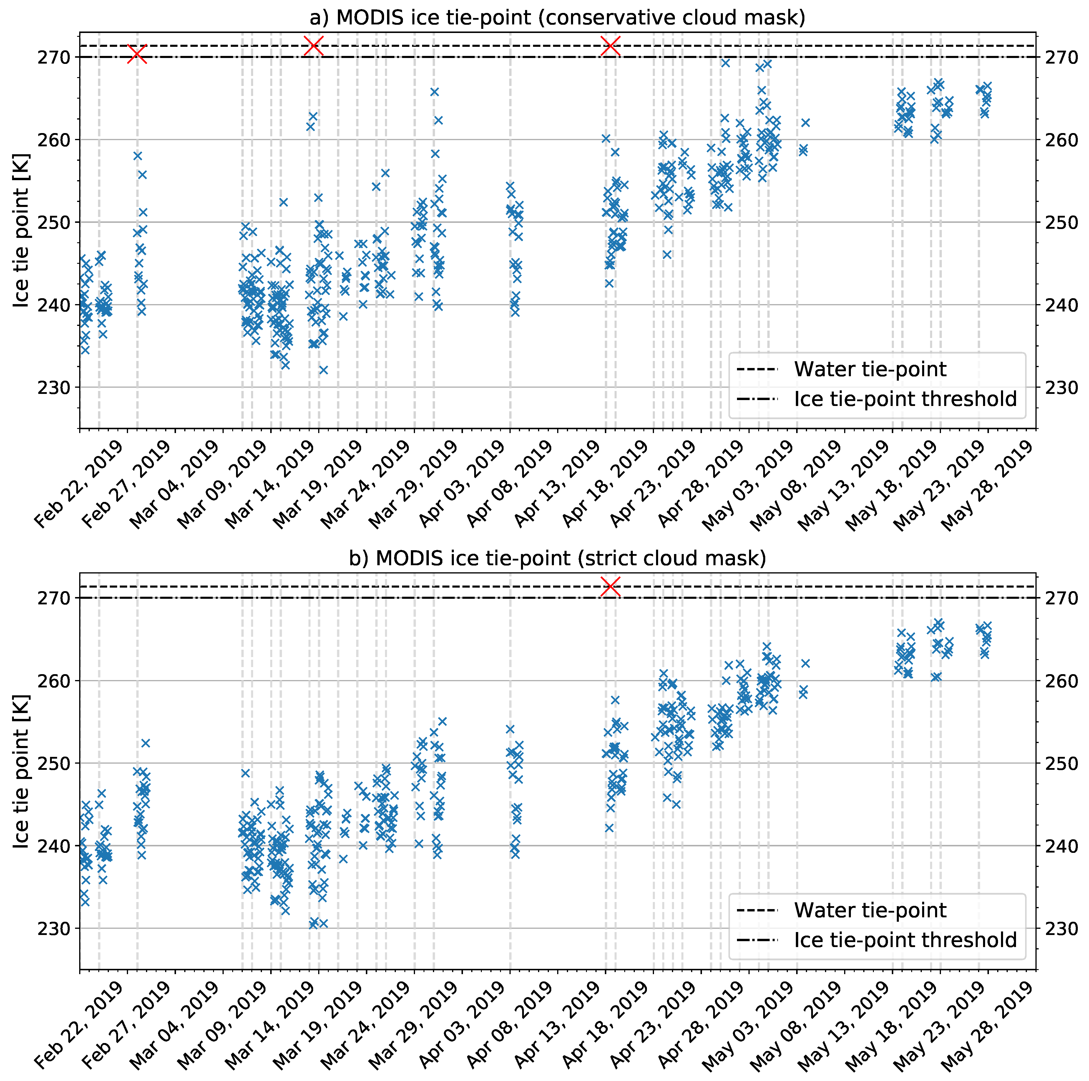
10]. The authors of [
10] apply a conservative cloud mask by masking only those pixels which the MODIS cloud mask (MYD35_L2, [
11]
https://ladsweb.modaps.eosdis.nasa.gov/archive/allData/61/MYD35_L2/, last access 12 September 2020) classifies as “confident cloudy”. We apply a stricter cloud mask by also discarding pixels which are labelled as “probably cloudy” and “probably clear”, thus only tolerating pixels which are labelled “confident clear”. Additionally, pixels over land, inland water and the open ocean are masked out by both cloud masks. The MYD29 data are sliced into granules which cover ~5 min. Each granule has a spatial dimension of 2030 km by 1354 km. The grid spacing is 1 km. Further details on the MYD29 dataset are given in [
10], at
https://nsidc.org/data/MOD29/versions/6 (last access 12 September 2020) and in the Algorithm Theoretical Baseline Document at
https://modis.gsfc.nasa.gov/data/atbd/atbd_mod10.pdf (last access 12 September 2020). For each Sentinel-2 scene, we downloaded all MODIS granules which intersected with the scene on the same day (997 granules in total). For the assessment of the MODIS ice tie-point (
Section 3.1) and the uncertainty estimates (
Section 3.3), all of these MODIS granules are used. For the intercomparison with the Sentinel-2 SIC (
Section 3.2), only the MODIS granules pertaining to the swath with the smallest time lag towards the Sentinel-2 scene are used. If the time lag exceeds 120 min, no intercomparison is done. For the merging, the granules are gridded to a north polar stereographic grid with the latitude of true scale at 70°N, also known and hereafter referred to as the NSIDC grid (
https://nsidc.org/data/polar-stereo/ps_grids.html, last access 12 September 2020). For the intercomparison with the Sentinel-2 SIC, they are resampled to a Transverse Mercator projection for consistency with the Sentinel-2 data.
2.2. ASI-AMSR2 Sea-Ice Concentration
The Advanced Microwave Scanning Radiometer 2 (AMSR2) aboard the Japan Aerospace Exploration Agency’s (JAXA’s) GCOM-W1 measures horizontally and vertically polarised electromagnetic radiation in seven microwave frequency bands between 6.9 GHz and 89 GHz. The polarisation difference at 89 GHz is used by the Arctic Radiation and Turbulence Interaction Study (ARTIST) Sea Ice algorithm (ASI). The ASI-AMSR2 SIC is provided as a daily gridded dataset at 6.25 km and 3.125 km grid spacing at
https://seaice.uni-bremen.de (last access 12 September 2020). For a better temporal consistency with the MODIS data, we use swath data processed internally. For the merged dataset, they are interpolated to the same projection and grid spacing as the MODIS data. For the intercomparison with the Sentinel-2 SIC, they are resampled to a Transverse Mercator projection for consistency with the Sentinel-2 data.
2.3. Sentinel-2 Reflectances
Sentinel-2 reflectances are used to create a reference SIC dataset for evaluation of the merged, MODIS and AMSR2 SIC. The EU Copernicus Sentinel-2A/B satellites were launched in June 2015 (Sentinel-2A) and March 2017 (Sentinel-2B). They follow a sun-synchronous orbit at 786 km altitude and 10:30 am equator crossing time. Their phase is shifted by 180°. Their payload, the Multispectral Instrument (MSI), features 13 bands in the visible and shortwave infrared spectral region. To obtain a reference dataset, we downloaded 79 cloud-free scenes from
https://scihub.copernicus.eu/ (last access 12 September 2020). We made sure that they are cloud-free by checking every scene visually.
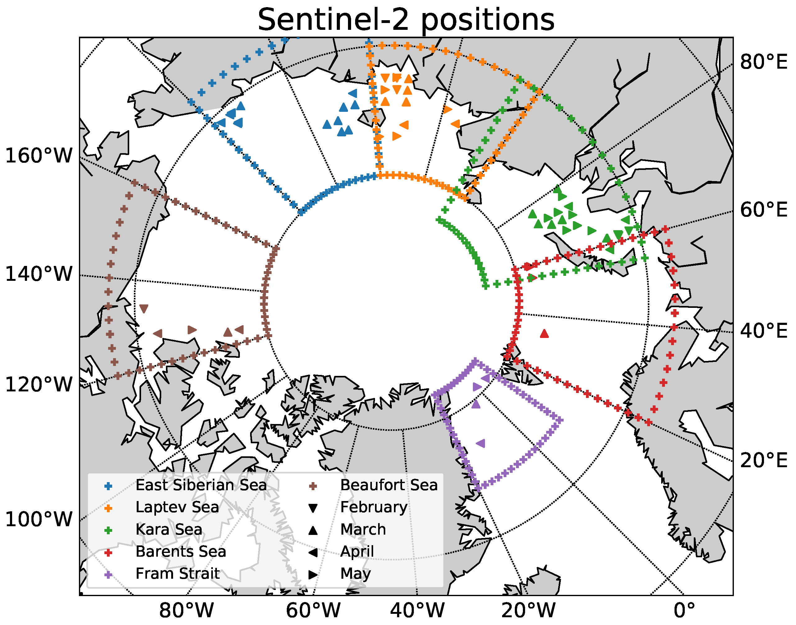
Figure 1 and
Table 1 offer a spatial and temporal overview over the scenes. Scenes with more than two hours time lag towards the next MODIS/AMSR2 overflight are not used for the intercomparison, but are included in the paper because of their possible relevance for other validation studies. The scenes were recorded in the East Siberian, Laptev, Kara, Barents, Beaufort Sea and in the Fram Strait between 22 February 2019 and 27th May 2019. The scenes comprise mainly first-year ice with smaller amounts of young ice. Ice-type maps based on Advanced Scatterometer (ASCAT) and AMSR2 data ([
12,
13,
14],
https://seaice.uni-bremen.de/multiyear-ice-concentration/, last access 12 September 2020) show some multiyear ice in the East Siberian, Fram Strait and Beaufort Sea (not explicitly shown here). For this study, Level 1 C reflectances at 665 nm (band 4) with a spatial resolution of 10 m are used. Level 1 C data are top-of-the-atmosphere reflectances which are projected onto a Universal Transverse Mercator projection.
2.4. MODIS Sea-Ice Concentration Retrieval
For the MODIS SIC retrieval, accurate knowledge of the background temperatures is crucial. The background temperatures, hereafter referred to as tie-points, are the reference temperatures which a pixel would have if it were covered completely by open water (water tie-point
) or covered completely by sea ice (ice tie-point
). For the tie-point retrieval, we follow the approach of the works in [
1,
8].
The choice of is straightforward: we assume that the open water is constantly at the freezing point of salt water, −1.8 °C. If it would be colder, the water would freeze to sea ice until thermal equilibrium is reached. If it would be warmer, it would melt the surrounding the sea ice and thereby cool down to the freezing point. However, until equilibrium is reached other water temperatures can also be observed, which is part of the uncertainty.
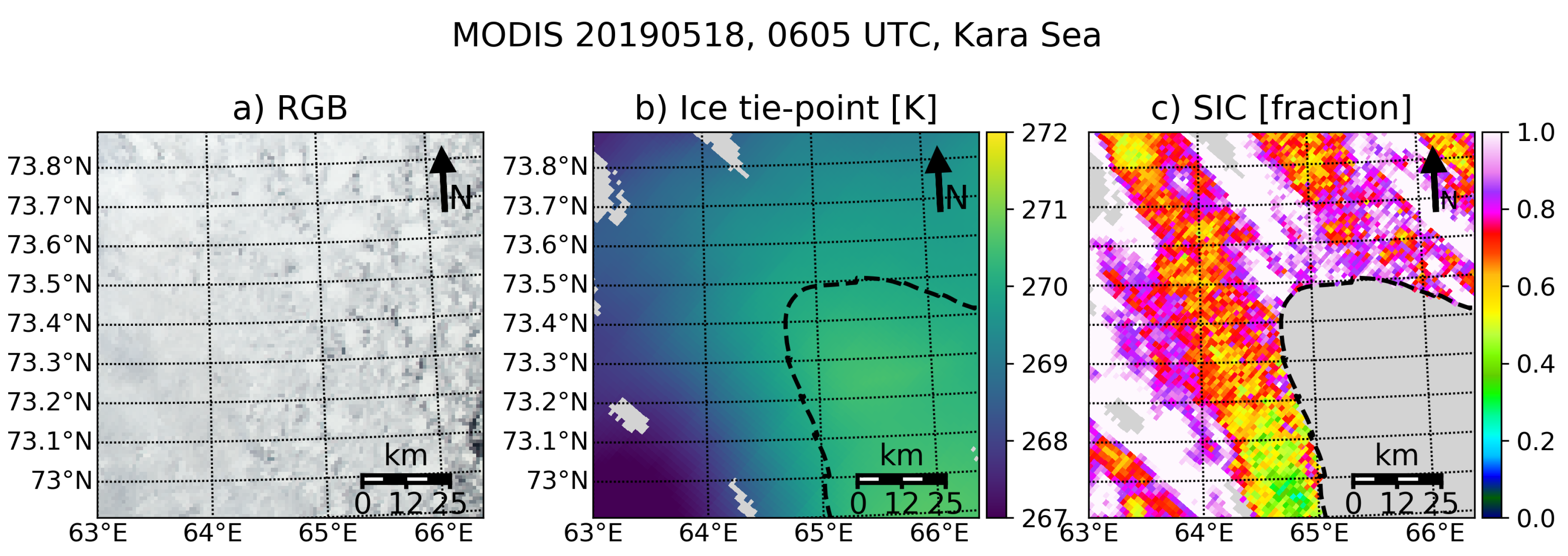
The choice of
is less straightforward. The IST follows the air temperature and thus has large spatial and temporal variability, which renders it impossible to choose an Arctic-wide fixed
. To account for the local variability, each pixel is assigned its own
. For this, the IST field is split into cells of 48 pixels by 48 pixels. We assume only linear IST variation within these cells. Each cell is split into 3 by 3 subcells of 16 pixels by 16 pixels. Within a subcell, we assume negligible IST variations. In the next step, the 25th percentile of the IST field in the subcell is selected as preliminary
, so that there are 9 preliminary
values per cell. Once the
are selected, a linear regression with two variables is performed within the cell to express the
as function of the x/y position within the cell:
where
x and
y are the indices of the respective pixel within the cell,
is
at this pixel, and
a,
b and
c are the regression coefficients. Subcells are discarded entirely if more than 70% of the pixels are covered by clouds and cells are discarded entirely if more than four subcells are discarded entirely. The authors of [
15] investigate the sensitivity of the retrieval towards the required fraction of cloud-free pixels within one subcell, the required number of valid subcells in one cell and the percentile for the estimation of
. They confirm that the initial settings are a reasonable choice. So far, the approach directly follows that in [
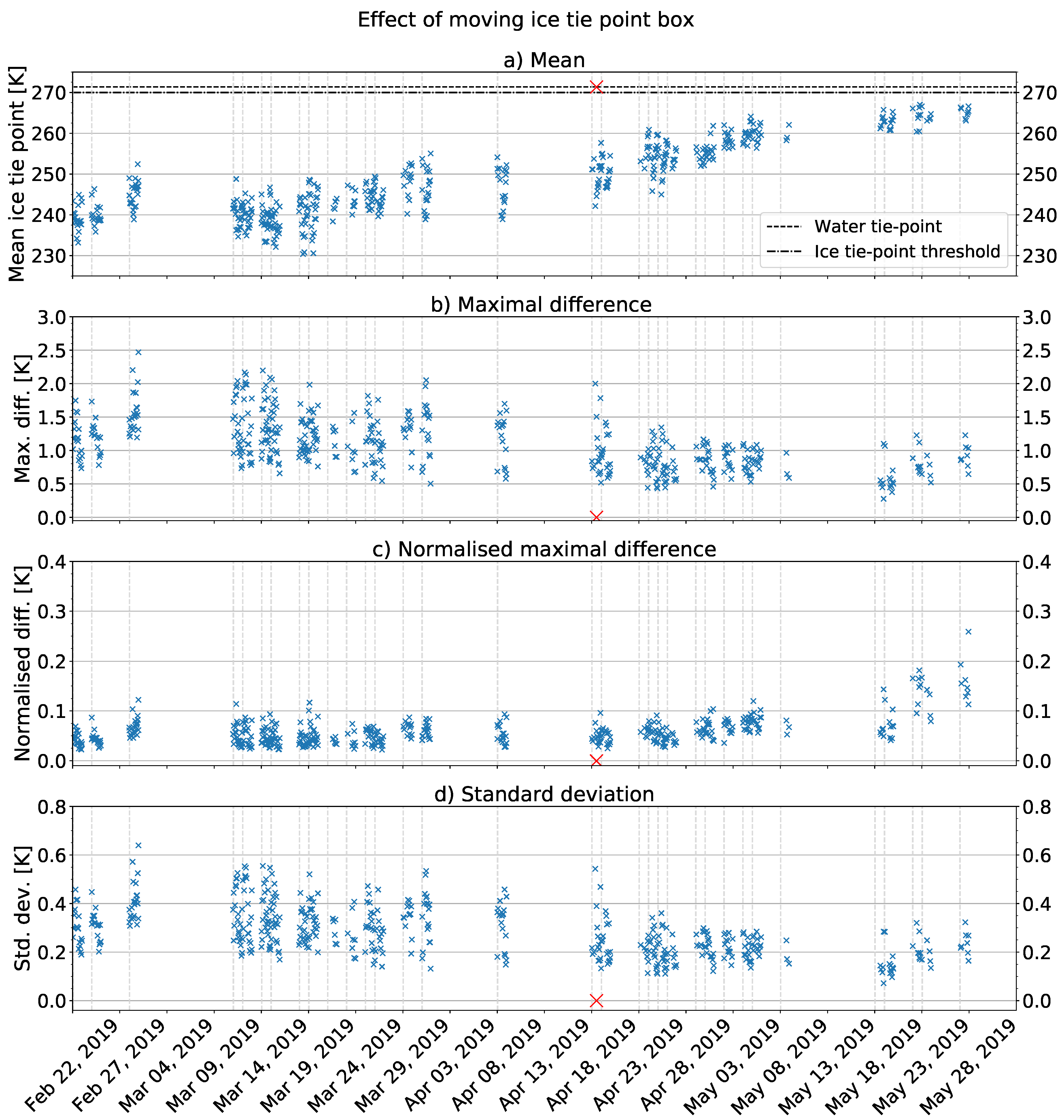
1]. They shift the cells by 48 pixels once the calculation is done, so that each pixel is covered once. As in [
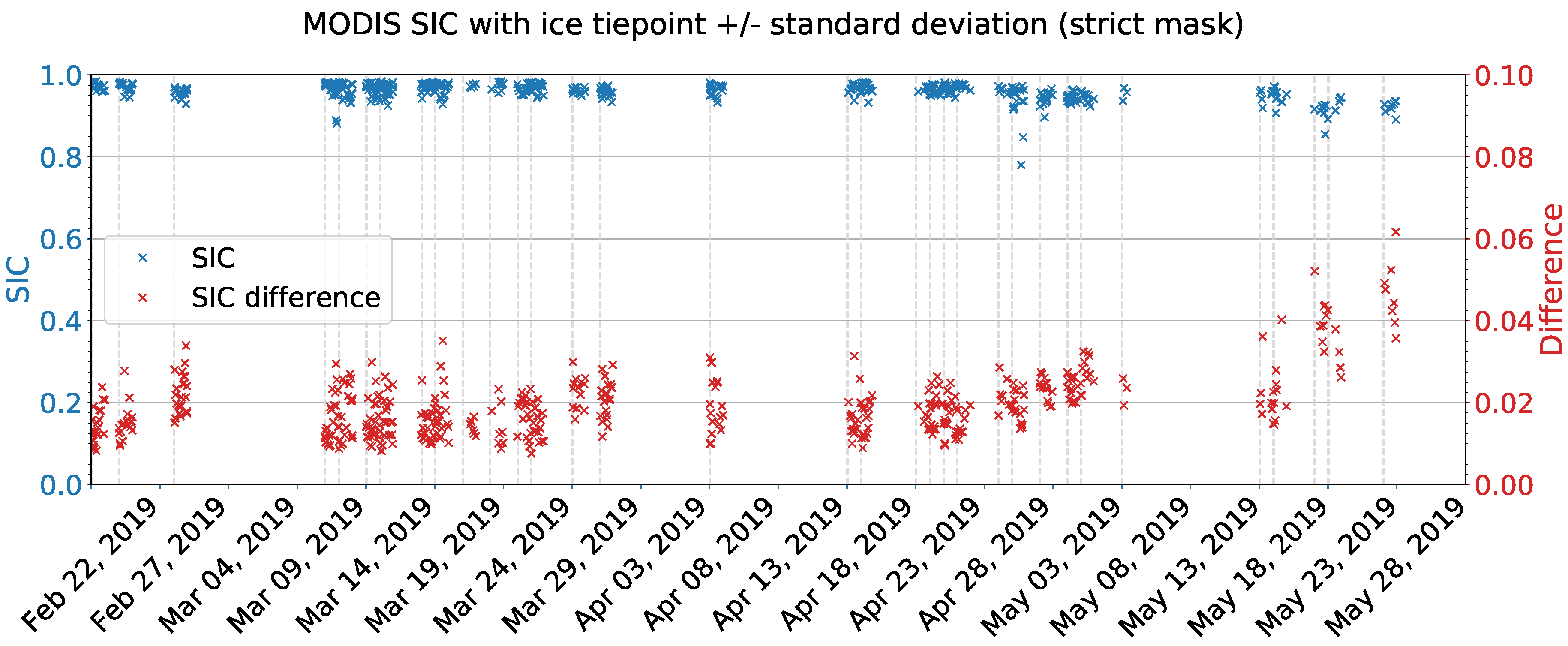
8], we shift the cell by 1 pixel before repeating the calculation, so that each pixel is covered 48 times. The mean of the 48 iterations is then selected as
. Our approach allows to use the standard deviation of the 48 iterations as estimate for the uncertainty of
. Once
for each pixel is determined, the IST is converted to SIC by linear interpolation:
No SIC retrieval is performed in the current version of our retrieval if exceeds 270 K.
The SIC calculation is performed on granule level. Subsequently, each granule is gridded to the NSIDC projection with 1 km grid spacing. Then, granules which belong to the same orbit are merged together, so that there is one MODIS SIC array per orbit.
2.5. Merging MODIS and AMSR2 Sea-Ice Concentration
After combining the gridded MODIS granules to one overflight, we select the corresponding AMSR2 overflight. As both platforms, Aqua and GCOM-W1, are part of the A-Train, the time lag is on the order of minutes. Our central assumption for the merging is that the MODIS SIC capture the variability at 1 km resolution correctly, but tend to underestimate the SIC due to the influence of thin ice thickness. Furthermore, they are limited by the presence of clouds. The AMSR2 SIC, on the other hand, are less sensitive to thin ice than the MODIS SIC, and thus retrieve the right magnitude at a spatial scale of 5 km and are available independently of cloud coverage. We thus tune the mean of the MODIS SIC in an area of 5 km by 5 km to match that of the AMSR2 data. This is done in the following way. First, the AMSR2 data are resampled/interpolated to a grid cell size of 1 km. Then, the difference between the mean MODIS SIC and the mean AMSR2 SIC in an area of 5 km by 5 km (i.e., 5 by 5 1 km-by-1 km pixels on the interpolated grid, not the original AMSR2 grid) is calculated:
where
and
are the mean MODIS and AMSR2 SIC in the respective 5 km by 5 km cell and
is their difference. This difference is now added to each MODIS pixel in this box such that it matches the mean of the AMSR2 pixels. In the final step, the cloud gaps are filled by the respective AMSR2 pixels:
Here,
is the merged SIC at the pixel with the coordinates
;
and
are the MODIS and AMSR2 SIC at this pixel, respectively, and
is defined as in Equation (
4). A similar approach has been used in [
16]. Different to them, we shift the 5 km by 5 km box by 1 pixel before the calculation is repeated for each pixel in the box. The mean is selected as merged SIC value. This mitigates the inaccuracy of choosing arbitrary starting positions for the merging, analogously to the approach which we chose for the
retrieval in
Section 2.4.
If the AMSR2 SIC are 100% in the entire scene, we allow SIC above 100% in some grid cells in order to resolve leads with reduced MODIS SIC which the AMSR2 did not show because they are overfrozen. By doing this the requirement of the merging procedure to keep the AMSR2 SIC mean (i.e., 100%) is fulfilled. In the end, however, the merged SIC is capped at 100%, which means that the means of the merged and the AMSR2 SIC are not entirely consistent in such cases. We accept this as a compromise for the enhanced potential to resolve leads. The above 100% SIC values before the truncation will be provided as additional information in our dataset.
2.6. Deriving Uncertainty Estimates
2.6.1. MODIS Sea-Ice Concentration Uncertainty
Several uncertainty-afflicted parameters enter the MODIS SIC retrieval. The MODIS SIC uncertainty,
, is given by Gaussian error propagation applied to Equation (
2):
where
,
and
are the uncertainty contributions of
,
and
, respectively. They are given by
where
,
and
are the uncertainties of
,
and
, respectively. We assume that
and
are equal to the measurement uncertainty of the MODIS IST, which amounts to 1.3 K [
10]. For
, we assume that it is equal to the standard deviation of the 48 iterations done for the retrieval of
in
Section 2.4. It is typically between 0.1 and 0.6 K (see Figure 4d).
2.6.2. Merged Sea-Ice Concentration Uncertainty
If MODIS data are available, the first case in Equation (
4) needs to be considered, and the merged SIC at the pixel with the coordinates (x,y) is given by
and
are basically two samples of the same dataset, only that
is the average MODIS SIC in the 5 km by 5 km around the pixel at the coordinates (x,y). We thus consider Equation (
9) to be a linear combination of the MODIS and AMSR2 SIC and calculate the uncertainty as
where
is the uncertainty of the merged SIC and
and
are the uncertainty contributions of the MODIS SIC and the AMSR2 SIC, respectively. As
and
are retrieved from different wavelength regimes and by different approaches, we consider them to be independent observations of the same quantity and thus scale the uncertainty by
.
and
are given by
where
is the MODIS SIC uncertainty as given by Equation (
5) and
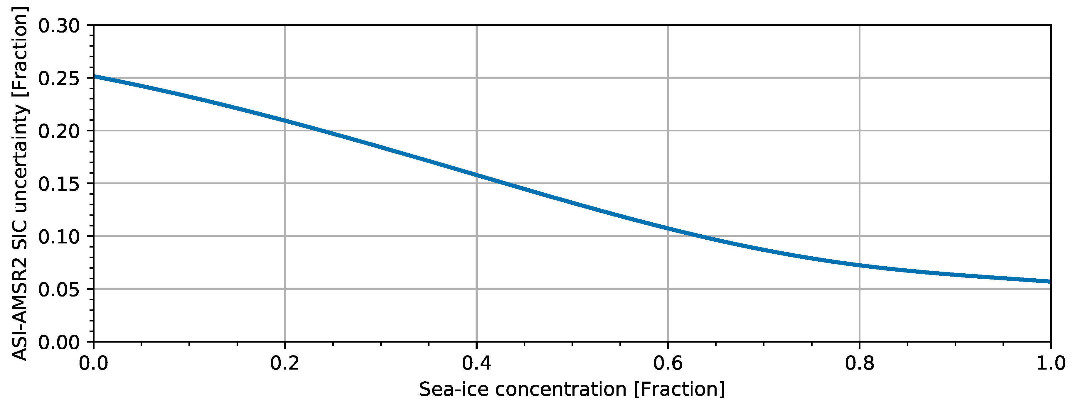
is the uncertainty of the AMSR2 SIC. We adopt the approach of the authors of [
17], who give
as a function of the AMSR2 SIC as shown in
Figure 2.
If MODIS data are not available for the merging, the merged SIC uncertainty is equal to the AMSR2 SIC uncertainty.
2.7. Sentinel-2 Sea-Ice Concentration
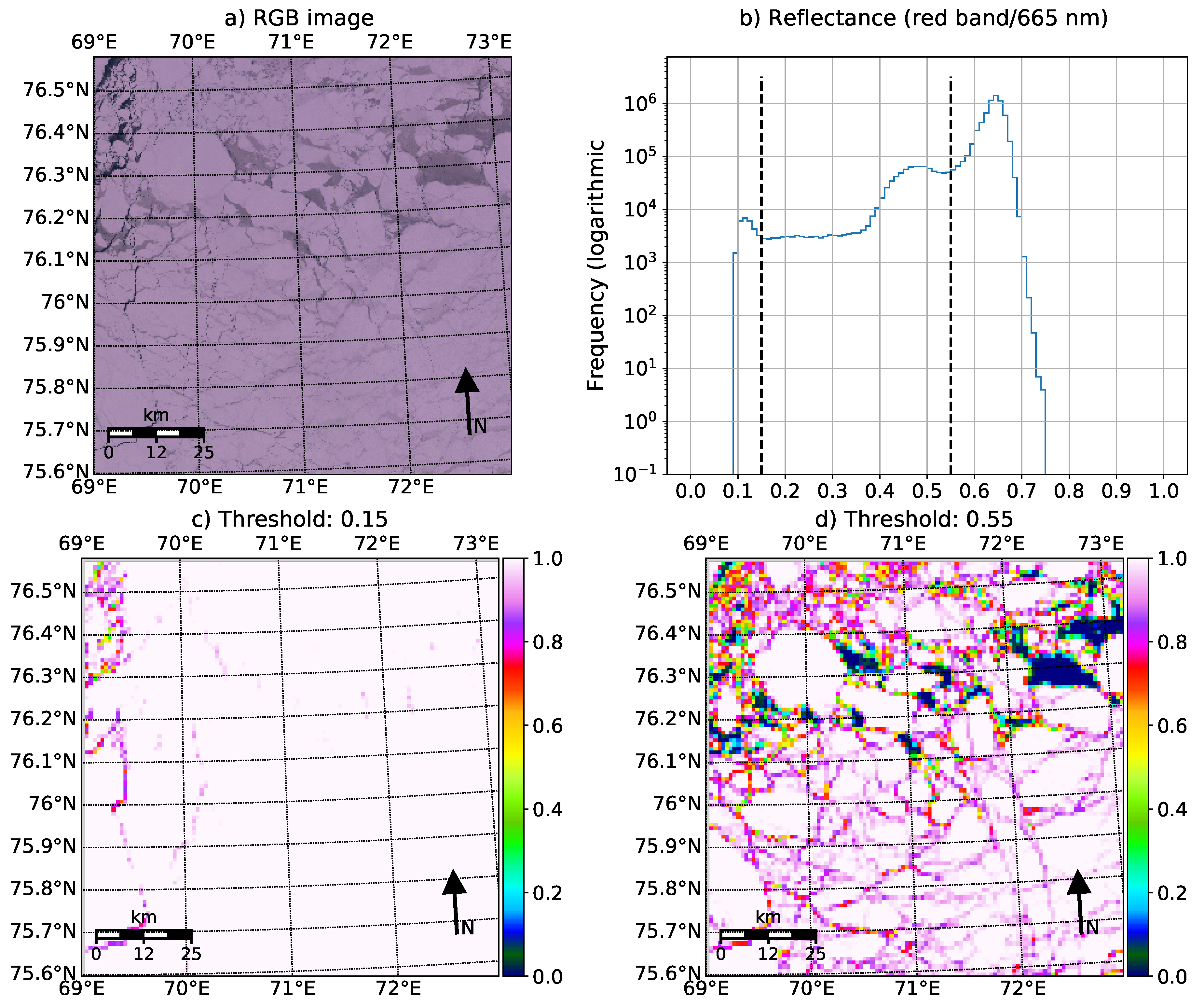
We classify the Sentinel-2 reflectances according to their frequency distribution (see the example in Figure 6b). The three bands from the visible spectrum (bands 2–4) are investigated. Histograms of all 3 bands (red/640 nm, green/560 nm and blue/490 nm) are evaluated for all 79 Sentinel-2 scenes. They show no notable difference for our purpose; all three bands enable a clear distinction between the thin and thick-ice classes if both classes are present and a clear distinction between ice and water if only thick ice is present. We decide to use band 4 (red/640 nm). The reflectances are classified into three classes: open water, thin ice and thick ice. As the ice peaks differ from scene to scene, we select specific thresholds for each scene instead of using a global threshold for each scene. If there are two peaks at the high end of the reflectance spectrum, both are treated as ice. We create two reference SIC datasets: One for which the thin-ice class is treated as ice and one for which it is treated as water. The SIC dataset where the thin ice is treated as water will be called thick-ice SIC as it comprises only thick ice. Consequently, the SIC dataset for which also thin ice is treated as ice will be called thin-ice dataset as it comprises thin and thick ice. The resolution of the binarised ice/water maps is 10 m and the desired resolution of the SIC dataset is 1 km. Thus, we assume that one SIC pixel (1 km) comprises 100 by 100 reflectance pixels. We select each pixel in the SIC array and assign it with the average of the surrounding 100 by 100 reflectance pixels, assuming that the SIC pixel is in the centre of the box. In this way, we obtain a SIC dataset at 1 km resolution from the 10 m reflectance dataset.
4. Discussion
The quality of the MODIS SIC which we present in
Section 3.1 depends crucially on the reliability of the cloud screening. Specifically, the MODIS cloud mask does not always identify thin clouds and fog correctly [
10]. We account for this by masking clouds strictly by only tolerating pixels which are flagged “confident clear”. This means that the confidence in the pixel being cloud-free is more than 99% [
21]. Even better cloud screening might be achieved with the Fuzzy Cloud Artifact Filter proposed by the authors of [
22], but using the MODIS cloud mask alone; this is the best we can do for cloud screening. Additionally, the merging procedure makes sure that even if there are unscreened clouds, the quality of the merged SIC is not much worse than that of the AMSR2 SIC, as we show in
Section 3.2 and
Figure 9.
Calculating the MODIS SIC, we find that changing the freezing point from −1.87 °C to −1.09 °C (corresponding to salinities of 34 and 20, respectively) only introduces a mean difference of 0.5%. A salinity of 20 is the lower limit of what one would expect for the marginal seas [
23]. It is higher in the Central Arctic, so that the small mean difference of 0.5% is already an upper limit of the actual error. The authors of [
15] find an even lower sensitivity of 0.2%. We thus consider the error introduced by the assumption of a constant freezing point as negligible. Additionally, not retrieving SIC for ice tie-points higher than 266.5 K in future makes sure that the dynamic range is large enough to be robust against small freezing point variations.
Both MODIS SIC and AMSR2 SIC are influenced by sea-ice thickness. The AMSR2 SIC underestimate a SIC of 100% by up to 50% for very thin ice (thinner than 6 cm), but are close to 100% SIC for ice thicker than this under the surface conditions of our study [
4]. The authors of [
5] confirm this by reporting SIC underestimations of 5% or less for sea-ice thicker than 10 cm. Other passive microwave SIC algorithms are affected more strongly by sea-ice thickness [
4,
5].
The MODIS SIC underestimation due to sea-ice thickness is not linked to a certain thickness. Instead, it depends on the distribution of sea-ice thickness. The MODIS SIC algorithm assumes a bimodal ice thickness distribution within the region used for the ice tie-point retrieval. If more than one sea-ice thickness class is present in this region, the ice tie-point will represent the ice-surface temperature above the thicker ice, while the thin ice will appear warmer due to the oceanic heat flux and will thus be retrieved as reduced SIC. This is desired by the authors of [
1] as their primary goal is to represent the thermal forcing of the atmosphere rather than the actual fraction of ice. We want to retrieve this fraction and thus tune the MODIS SIC to the mean of the AMSR2 SIC.
A situation with inhomogeneously distributed sea-ice thickness as described above can happen throughout the winter season, while sea ice which is thin enough to appear as reduced SIC in the AMSR2 SIC is not expected that often, especially in winter then the large temperature contrast between ocean and air lets the ice grow quickly. We thus consider the AMSR2 SIC to be less dependent on sea-ice thickness than the MODIS SIC, which is again an argument for tuning the MODIS SIC to match the mean of the AMSR2 SIC.
The main benefit of including the MODIS data is the higher potential for identifying leads. Generally, it is debatable whether an overfrozen lead should be shown as reduced SIC, as strictly speaking the SIC should be 100% instantly when the lead starts to refreeze. For most applications, e.g., heat flux calculation or navigation, the presence of leads is very relevant. A calculation in [
24] shows that for thick ice the heat flux would be ~9 Wm
−2 for 99% SIC and 5 Wm
−2 for 100% SIC. In a 1 km grid cell of our dataset, this would correspond to a difference of 4 MW. We see this and the importance of leads for navigation as a sufficient argument for keeping the leads as reduced SIC in our merged dataset. The benefit of keeping the leads is also reflected in the higher open-water extent of the merged and MODIS SIC compared to the AMSR2 SIC.
For lead retrieval only, the MODIS SIC would be more suitable than the merged SIC. However, our main goal is to have a dataset which does not only allow lead identification, but also offers spatial continuity. We therefore see our dataset as a compromise where a part of the lead information from the MODIS data is lost, but we judge the spatial continuity as valuable enough to accept this as a trade-off. For users who are mainly interested in leads, the MODIS SIC will be provided along with the merged SIC in a future version of our dataset.
Both MODIS and AMSR2 SIC are strongly influenced by melt ponds. We do not consider this relevant for our study here since we do not cover the melt season, but it makes MODIS SIC retrieval in summer impossible, especially if we discard pixels with ice tie-points above 266.5 K as derived in
Section 3.3. The merged SIC are thus only available between October and May.
We do not compare our merged SIC to passive microwave SIC. The reason for this is that the main advantage of our product over the well-established passive microwave SIC algorithms is the finer resolution. As the ASI-AMSR2 SIC have the finest spatial resolution of all passive microwave SIC algorithms, we expect the ASI-AMSR2 SIC to yield an open-water extent (the metric which we use to show the advantages of the merged SIC) which is closer to that of the Sentinel-2 reference SIC than for the other passive microwave algorithms. Showing that the open-water extent of our merged SIC is closer to the Sentinel-2 open-water extent than that of the ASI-AMSR2 SIC does thus immanently show that the merged SIC are also better compared to the other passive microwave SIC with their even coarser spatial resolution. As we preserve the mean of the ASI-AMSR2 SIC, previous comparisons of ASI-AMSR2 SIC to alternative SIC products [
24,
25,
26,
27] are also valid for our product in terms of potential biases, although the variability might be different.
The selection of Sentinel-2 scenes for evaluation could introduce a bias into our dataset as we are (a) limited to daylight conditions, (b) limited to the marginal seas and (c) limited to temporally unevenly sampled scenes. Our results are thus only representative for these conditions and regions, they should not be interpreted as an assessment of the Arctic-wide SIC transition from late Winter to early Summer. However, the 66 reference scenes cover a fair amount of different ice conditions and a higher than average percentage of intermediate ice concentrations due to their location in the marginal seas. Low and intermediate SIC retrievals are in general more challenging and have higher uncertainties than the close to 100% SIC in the central Arctic. Thus, we do not expect worse results for such cases.
For evaluation, the authors of [
15] compare the MODIS SIC with SIC derived from aircraft measurements and find an error of ±10% in April. Comparison with SSM/I data, also done by [
15], yields a linear regression error of ±7%. The MODIS SIC uncertainties derived by us are on average lower than the ones from the work in [
15], but are larger (up to 20%) in some cases. In May, they range from 10% to 35%, i.e., they are larger than the ones in [
15]. However, as the values in April, when the work in [
15] was done, agree rather well, we conclude that our MODIS SIC uncertainty estimates are in the range of what we expect from the literature.
We make a quite simple approach for estimating the AMSR2 SIC uncertainty by simply assuming them as a function of the SIC after [
17], yielding uncertainties between 5% and 10%. The accuracy of the AMSR2 SIC and 12 other passive microwave SIC algorithms has been assessed by [
26]. They report accuracies between 3.1% and 8.1% compared to a reference dataset of 75% SIC in winter (
Table 2b in [
26]). The accuracy of ASI given by [
26] is 3.9%. Our uncertainty estimates for the merged SIC during spring are mostly at the upper end of the range of the passive microwave SIC algorithms given in [
26], but higher in summer. However, the finer spatial resolution of our dataset has to be taken into account as an additional advantage. We thus judge our merged SIC uncertainty estimates as acceptable.
5. Summary
In this study, we first provide an assessment of the sensitivity of the MODIS SIC towards the choice of the ice tie-point, which is an essential parameter for the MODIS SIC retrieval. This is done by varying the starting position of the region which is used for the ice tie-point retrieval. This yields an ensemble of up to 48 possible MODIS ice tie-points, the mean of which is selected as final ice tie-point and the standard deviation of which is used as an estimate of the tie-point uncertainty. We find that the standard deviation averaged over all seasons is 0.33 K, which corresponds to 1.7% of the dynamic range. Converted to SIC, this yields an uncertainty of on average 1.9% and at maximum 6.2%. We mitigate this uncertainty as much as possible by varying the region for the ice tie-point retrieval and taking the average as ice tie-point.
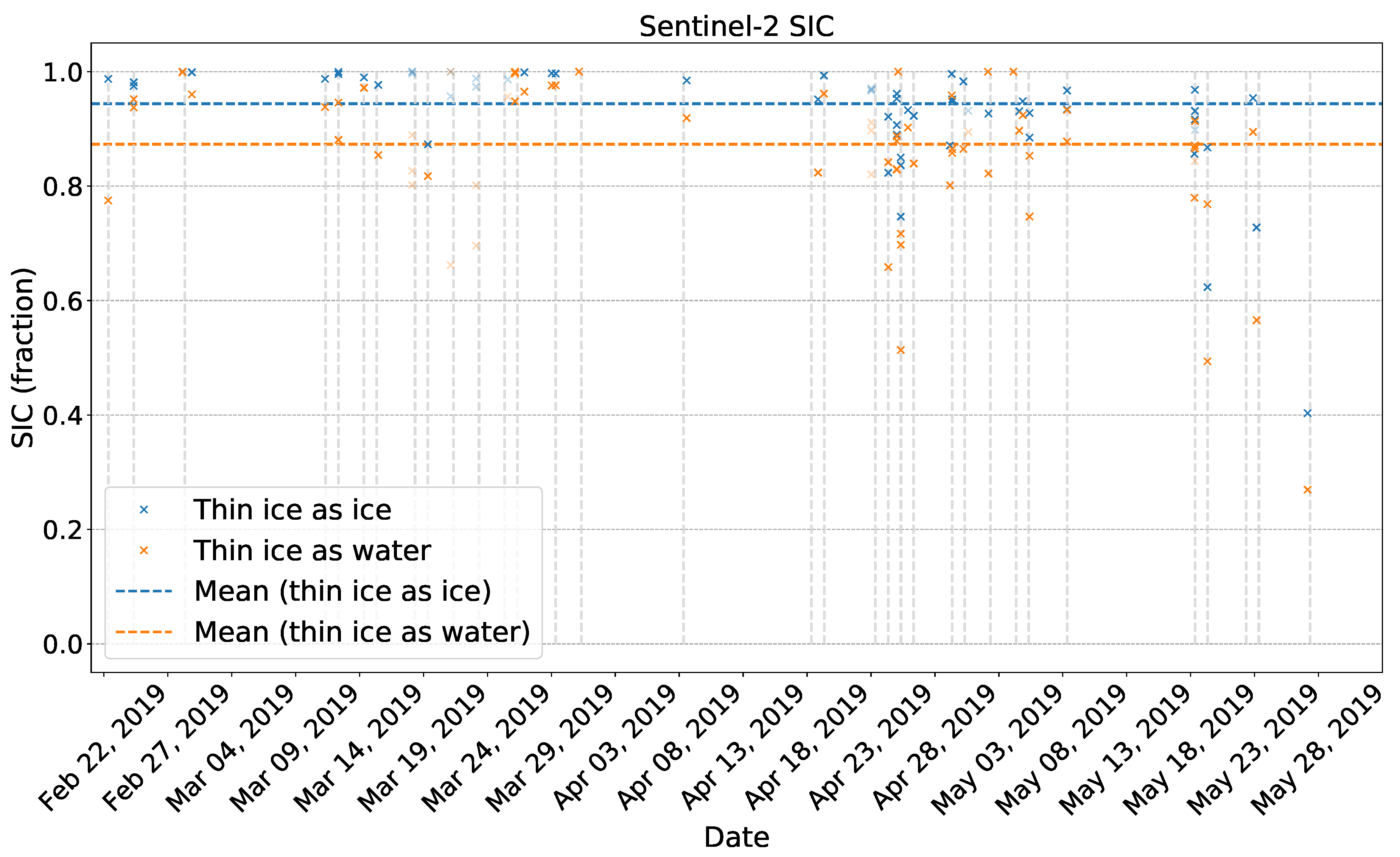
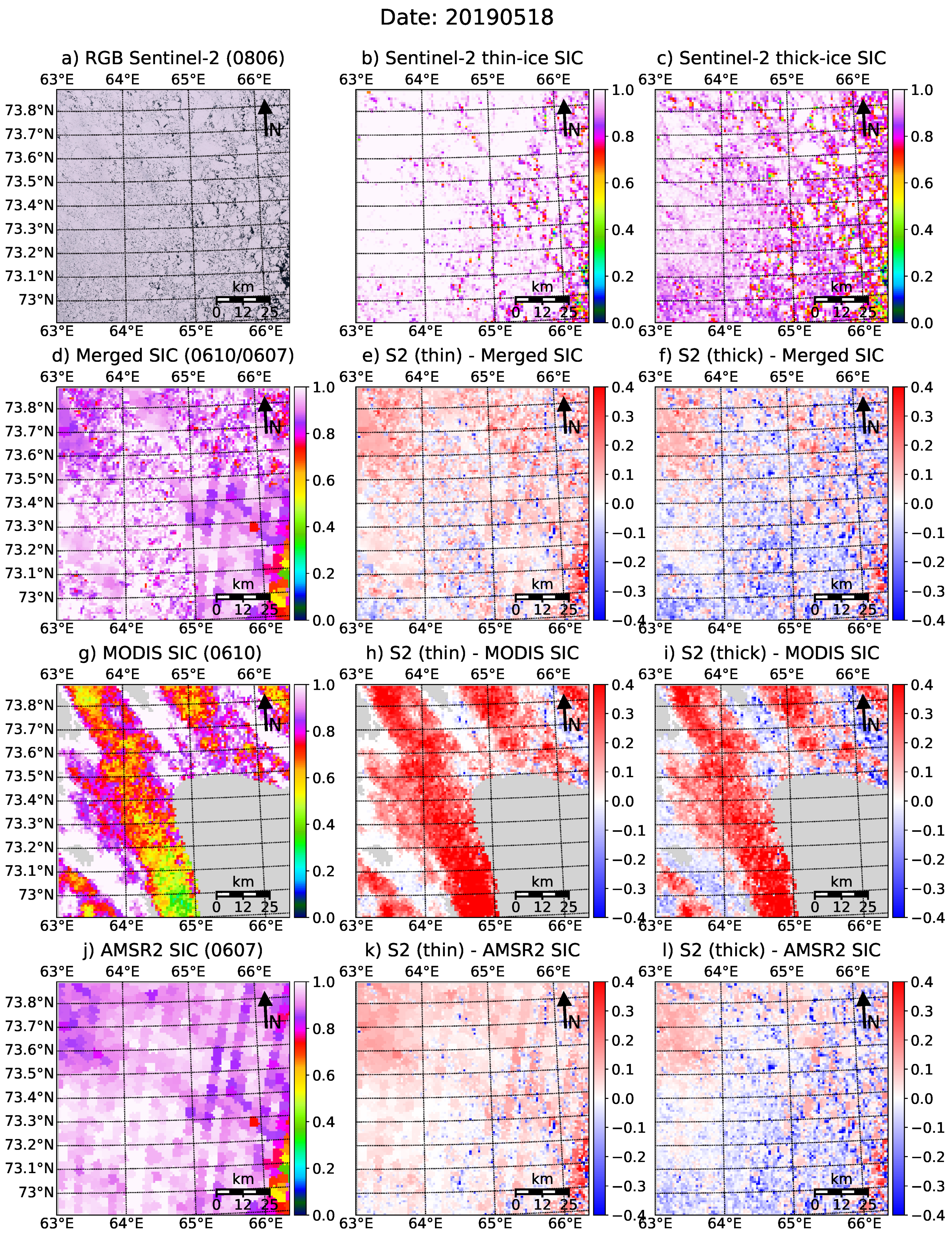
Furthermore, our study presents an intercomparison of our merged SIC dataset and its constituents—the MODIS and AMSR2 SIC—with independent reference data. To this end, we produce a reference SIC dataset from 79 Sentinel-2 scenes by classifying the reflectances into water, thin ice and thick ice. The scenes cover the period from February 22nd to May 27th and are located in the Arctic marginal seas and in the Fram Strait (
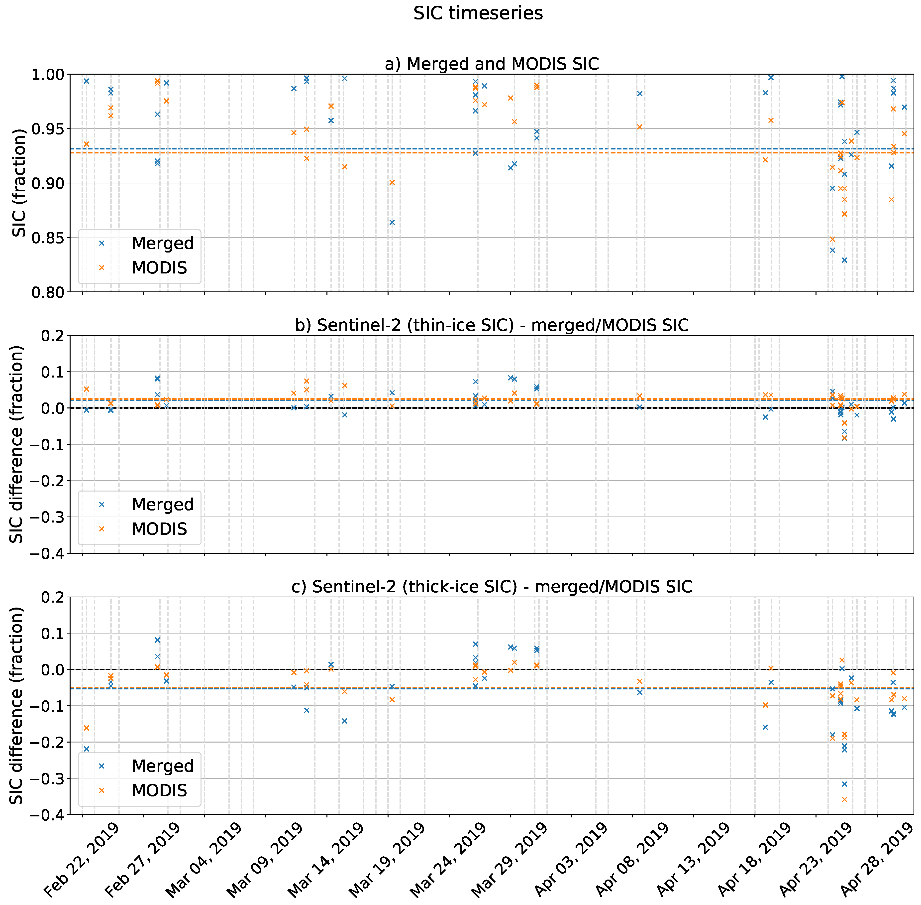
Figure 1). They are mostly dominated by a compact sea-ice cover and leads, but also comprise open-water areas. In theory, thin ice is part of the ice cover and should be reproduced as high SIC by a SIC retrieval. Thus, treating thin ice as ice (thin-ice SIC) is the primary reference dataset. However, to evaluate the sensitivity of our SIC retrievals to thin ice, we created a second reference SIC dataset for which we included the thin ice in the open water class and only consider thick ice as ice (thick-ice SIC). Treating only thick ice as ice (thick-ice SIC) yielded a mean Sentinel-2 SIC of 87.3%, and treating thin and thick ice as ice (thin-ice SIC) yielded a mean SIC of 94.4%. In the latter case, the standard deviation decreases from 13.2% (thick-ice SIC) to 9.2%. The mean merged and MODIS SIC are 93.1% and 92.8%, respectively, which means that there is closer agreement with the thin-ice SIC than with the thick-ice SIC. Thus, both retrievals correctly identify thin ice as ice and only show a small underestimation of about 1% due to the presence of thin ice for the 66 Sentinel-2 reference scenes used for the intercomparison. The RMSD between the merged and MODIS SIC is 5%, which means that the algorithms do yield different results despite the small bias. We further investigate this by analysing one scene with good-quality MODIS SIC and one scene with poor-quality MODIS SIC. In the first case, the combination of the fine resolution of the MODIS SIC and the magnitude of the AMSR2 SIC used for the merged SIC retrieval allows better representation of the reference data than with either dataset alone. In this scene, the merged SIC has a smaller difference and a smaller RMSD than the MODIS SIC compared to the thin-ice reference dataset, while, at the same time, the fine resolution causes an open-water extent which is closer to the thin-ice SIC than the MODIS or AMSR2 SIC. In the poor-quality MODIS SIC case, an unscreened cloud and high ISTs deteriorate the quality of the MODIS SIC. This is mitigated by the merging, so that the result has a similar quality as the AMSR2 SIC alone, however likely not improving it.
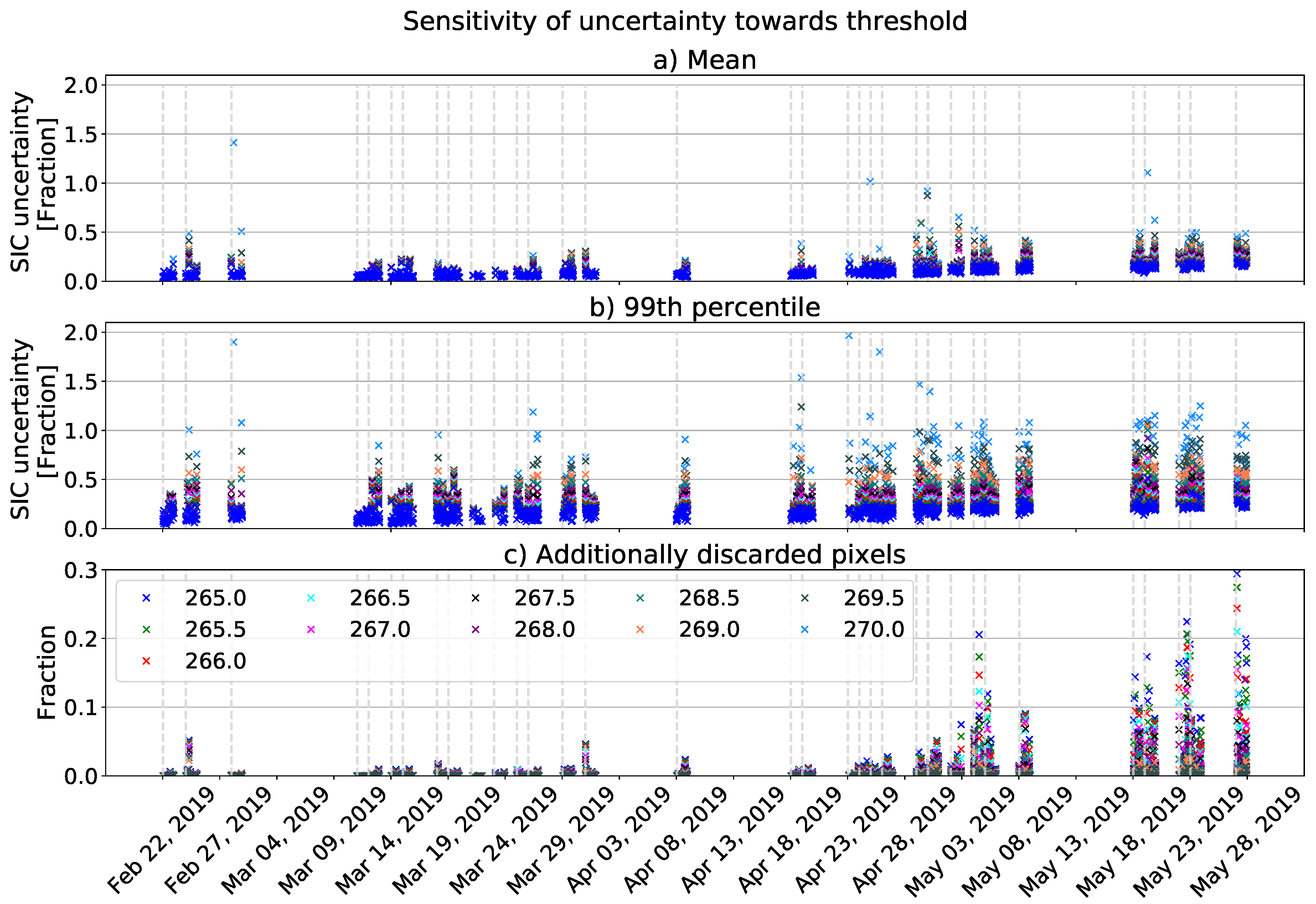
In the third part of our study, we give an uncertainty estimate for the merged, MODIS and AMSR2 SIC. Uncertainties are derived by Gaussian error propagation based on the ice and water tie-point uncertainties and the observational uncertainty for the MODIS SIC and by expressing them as a function of the SIC according to [
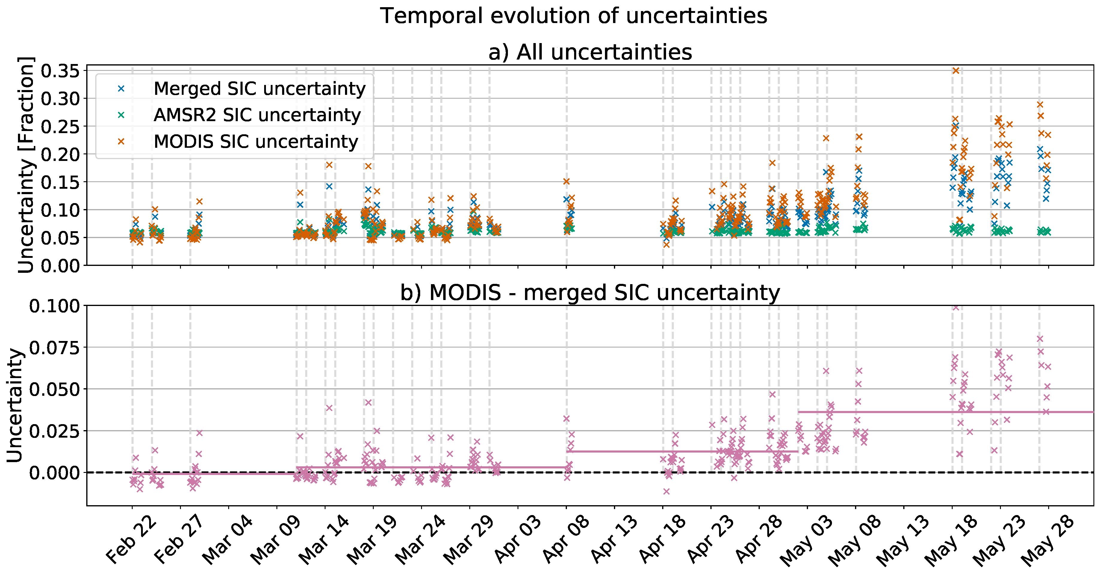
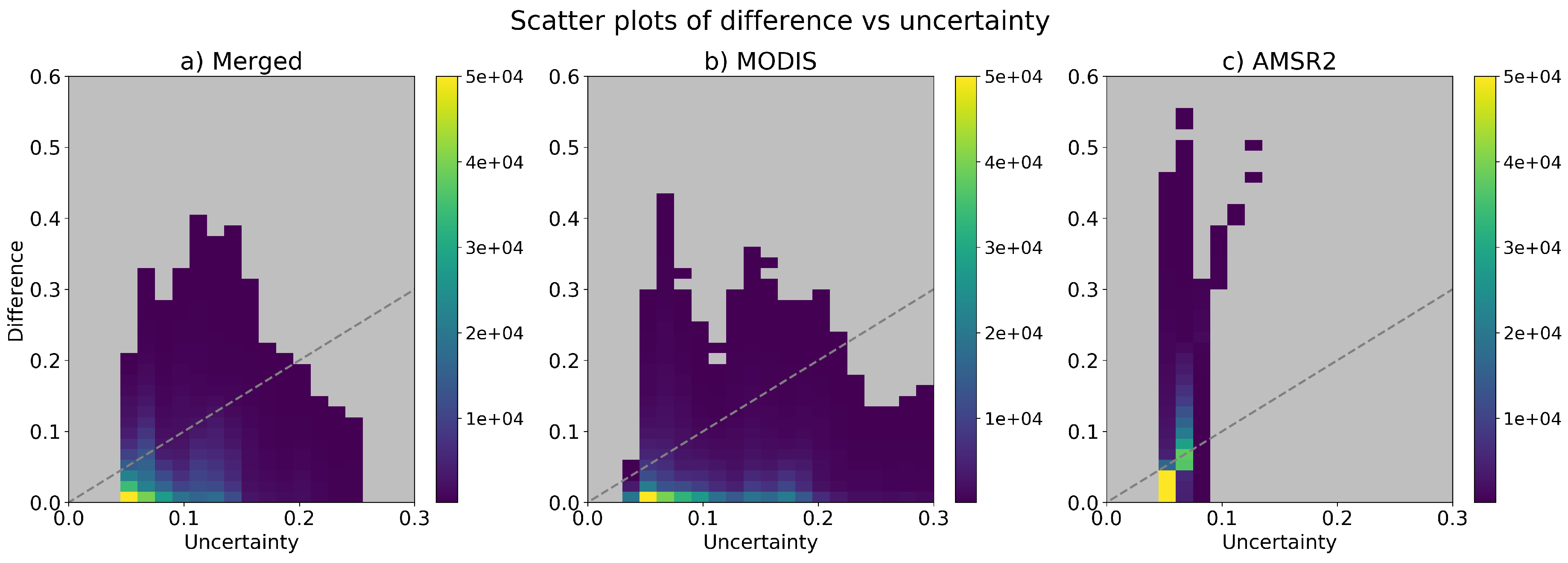
17] for the AMSR2 SIC. Gaussian error propagation then yields the merged SIC uncertainty. We use those uncertainties to determine a sanity threshold for the MODIS ice tie-point above which retrieval of meaningful MODIS SIC is no longer possible. A threshold of 266.5 K, i.e., about 5 K below the seawater freezing point, is chosen as a compromise between keeping the uncertainties small and discarding as few pixels as possible. A time-series of the uncertainties shows that the evolution of the merged and MODIS SIC uncertainty is mostly synchronous and between 5% and 15% until mid April, when the MODIS SIC uncertainty gets larger than the merged SIC uncertainty. In May, the average merged SIC uncertainty is 18% while the average MODIS SIC uncertainty is 25%. The AMSR2 SIC is constantly between 6% and 8% throughout the entire period, which is mostly due to our selection of scenes with high SIC and the much simpler uncertainty assumption for the AMSR2 SIC, which does not take atmospheric variability into account. Last, we compare our uncertainties to the differences between the merged, MODIS and AMSR2 SIC and the Sentinel-2 reference SIC (classifying thin ice as ice). We find that in most cases (≈80%) our uncertainties are higher than the differences. We conclude that our uncertainties are a conservative estimate of the actual uncertainty.
7. Outlook
Evaluation in winter and in the Central Arctic could be done using SAR data. Retrieving SIC from SAR data is challenging and would require more analysis than we can provide in the framework of this paper. We recommend it as a direction for future research, especially as we expect a good performance of our merged dataset due to the large thermal contrast between water and sea ice in winter.
The meaningful use of MODIS thermal infrared data is limited to winter and spring conditions. In summer, visible data can provide similar fine-resolution data which can be used for the merging. Especially as most of the ship traffic is in summer, this would be a valuable extension of our dataset.
A study comparing our dataset to the coarser-resolution passive microwave SIC algorithms based on the 19 GHz and 37 GHz frequency channels could be done to demonstrate the advantage of the fine resolution of the merged SIC over these algorithms.
The MODIS instruments aboard Aqua and Terra have exceeded their design lifespans and successor missions like NASA’s VIIRS (since 2011) aboard the Suomi NPP satellite or the SLSTR and OLCI on ESA’s Sentinel-3A (since 2016) and Sentinel-3B (since 2018) satellites are already operational. Visible and thermal infrared data from these satellites can assure continuity of our merged dataset once MODIS ceases operation. A possible follow-up for the AMSR2 passive microwave data is the Copernicus Imaging Microwave Radiometer (CIMR) whose launch is scheduled for 2028.


