Article

From Drones to Phenotype: Using UAV-LiDAR to Detect Species and Provenance Variation in Tree Productivity and Structure

1
School of Natural Sciences & ARC Training Center for Forest Value, University of Tasmania, Hobart 7001, Australia
2
School of Technology, Environments and Design, University of Tasmania, Hobart 7001, Australia
3
Greening Australia, Mount Nelson 7007, Australia
*
Author to whom correspondence should be addressed.
Remote Sens. 2020, 12(19), 3184; https://doi.org/10.3390/rs12193184
Submission received: 23 September 2020 / Accepted: 27 September 2020 / Published: 29 September 2020
(This article belongs to the Special Issue Feature Paper Special Issue on Forest Remote Sensing)

Abstract

:
The use of unmanned aerial vehicles (UAVs) for remote sensing of natural environments has increased over the last decade. However, applications of this technology for high-throughput individual tree phenotyping in a quantitative genetic framework are rare. We here demonstrate a two-phased analytical pipeline that rapidly phenotypes and filters for genetic signals in traditional and novel tree productivity and architectural traits derived from ultra-dense light detection and ranging (LiDAR) point clouds. The goal of this study was rapidly phenotype individual trees to understand the genetic basis of ecologically and economically significant traits important for guiding the management of natural resources. Individual tree point clouds were acquired using UAV-LiDAR captured over a multi-provenance common-garden restoration field trial located in Tasmania, Australia, established using two eucalypt species (Eucalyptus pauciflora and Eucalyptus tenuiramis). Twenty-five tree productivity and architectural traits were calculated for each individual tree point cloud. The first phase of the analytical pipeline found significant species differences in 13 of the 25 derived traits, revealing key structural differences in productivity and crown architecture between species. The second phase investigated the within species variation in the same 25 structural traits. Significant provenance variation was detected for 20 structural traits in E. pauciflora and 10 in E. tenuiramis, with signals of divergent selection found for 11 and 7 traits, respectively, putatively driven by the home-site environment shaping the observed variation. Our results highlight the genetic-based diversity within and between species for traits important for forest structure, such as crown density and structural complexity. As species and provenances are being increasingly translocated across the landscape to mitigate the effects of rapid climate change, our results that were achieved through rapid phenotyping using UAV-LiDAR, raise the need to understand the functional value of productivity and architectural traits reflecting species and provenance differences in crown structure and the interplay they have on the dependent biotic communities.

1. Introduction

Emerging advances in unmanned aerial vehicles (UAVs) and miniaturization of sensors allow the acquisition of ultra-high-resolution data (>1000 points/m2) for phenotyping and studying biological processes at the individual tree level in ways never before imagined [1,2]. Phenotyping is the first step in unravelling the genetic control of traits of ecological and economical significance. This understanding is important as the genetic variation in traits among populations often reflects plant adaptation to environmental variation [3], and allows the prediction of population responses to selection, be it artificial (breeding) or natural (evolutionary response) [4]. In the case of quantitative genetics, such studies require phenotyping a large number of individuals to allow the accurate estimation of genetic parameters, such as provenance differences and heritability. Achieving the required large-scale phenotyping is particularly difficult and costly for large, long-lived lifeforms such as trees. While traditional phenotypic traits, such as tree height, can be quantified using remote sensing with greater speed and precision than on-ground measurements [5], dense UAV-derived point clouds allow the estimation of difficult-to-measure traits (e.g., above-ground biomass or crown architectural traits) and the development of novel crown shape and density traits.
While there are obvious advantages in the use of remote sensing for phenotyping forest trees [4], its uptake in genetics and breeding studies has been slow. Recently, UAV technologies have been used for phenotyping genetic trials of Norway spruce (Picea abies) through RGB-derived (red, green, blue) photogrammetric point clouds [6]. The authors attempted to estimate tree height, intra-annual height increment and phenology at an individual tree level but were only able to accurately estimate tree height using the RGB-derived point cloud. Although the use of photogrammetric point clouds has become increasingly common in forest tree studies, higher rates of canopy penetration are achieved using light detection and ranging (LiDAR) [7]. For example, UAV-LiDAR was used to quantify structural differences among three genetic populations of Douglas-fir (Pseudotsuga menziesii) with different predicted genetic gain using area-based [8] and individual tree-level [9] analysis. Results showed high concordance between predicted population rankings and derived traits from the dense LiDAR point cloud, such as tree height, crown dimensions and leaf area.
In the field of ecological restoration, remote sensing of tree architecture and productivity traits is important for large-scale monitoring, as these traits are known to influence ecosystem services and functions [10]. However, the challenge remains to understand how species and provenances differ in these traits, especially as there is now a paradigm shift towards the development of climate-resilient restoration plantings using local and non-local species and provenances [11]. This is important as the extent to which provenances are locally adapted affects provenance choice and translocation decisions, and is a fundamental concept that underpins many of the provenancing strategies designed to develop resilient restoration plantings in the face of climate change [12]. The other relevant component of quantitative genetic variation is the within provenance variation which, in the case of wild seed collections, is reflected in the trait differences between individual open-pollinated seed lots (hereafter called families) from the same population [13]. With appropriate assumptions, this family-level variation allows insights into the additive genetic variation existing within populations and the narrow-sense heritability (i.e., h2) of traits [13]. Understanding genetic variation at this level is likely to uncover whether local provenances have sufficient genetic variation in functional traits to respond to climate change [14].
We here present one of the first studies investigating quantitative genetic variation in traditional and novel traits derived from UAV-borne LiDAR data. We focus on key structural traits associated with tree architecture and productivity estimated for two Eucalyptus species regularly used for ecological restoration of temperate woodland ecosystems in south-eastern Australia. Using a multi-provenance common-garden experiment embedded within the broader restoration plantings, we develop and test a two-phased analytical framework to reveal signals of local climate adaptation. Our results highlight new opportunities for high-throughput phenotyping using remote sensing techniques and the quantification of novel tree architecture and productivity traits of putative functional value in forest ecosystems.

2. Materials and Methods

2.1. Study Site

The present study used field and remotely sensed data from a common-garden trial established at Dungrove (592 m elevation, latitude −42.2733°, longitude 146.8941°) in southern Tasmania, Australia (Figure 1a). We focused on the pedigreed eucalypt treatments of the ‘ecology trial’ reported in Camarretta et al. [15], which comprised three treatments of Eucalyptus pauciflora and Eucalyptus tenuiramis planted as monoculture or mixed species. The seed material was collected during the 2009/2010 austral summer, and at the time of trail establishment (October 2010), seedlings were approximately 10 months old. For each focal eucalypt species, sixty open-pollinated families were sampled from each of the 10 provenances across their native distribution in Tasmania (i.e., 60 families represented per species; Table S1). Families were randomized within each treatment irrespective of provenance and planted as single-tree plots. In the case of the mixed eucalypt treatment, species were alternated along cultivation rows, where each single-tree plot was randomly allocated a family irrespective of provenance. For the monoculture treatment, two provenance trial designs were overlayed. In each randomized complete block design, provenances and families were allocated randomly along rip lines. Each treatment was replicated eight times across the trial site and planted as a complete randomized block design.

2.2. UAV-LiDAR Collection, Processing and Trait Calculation

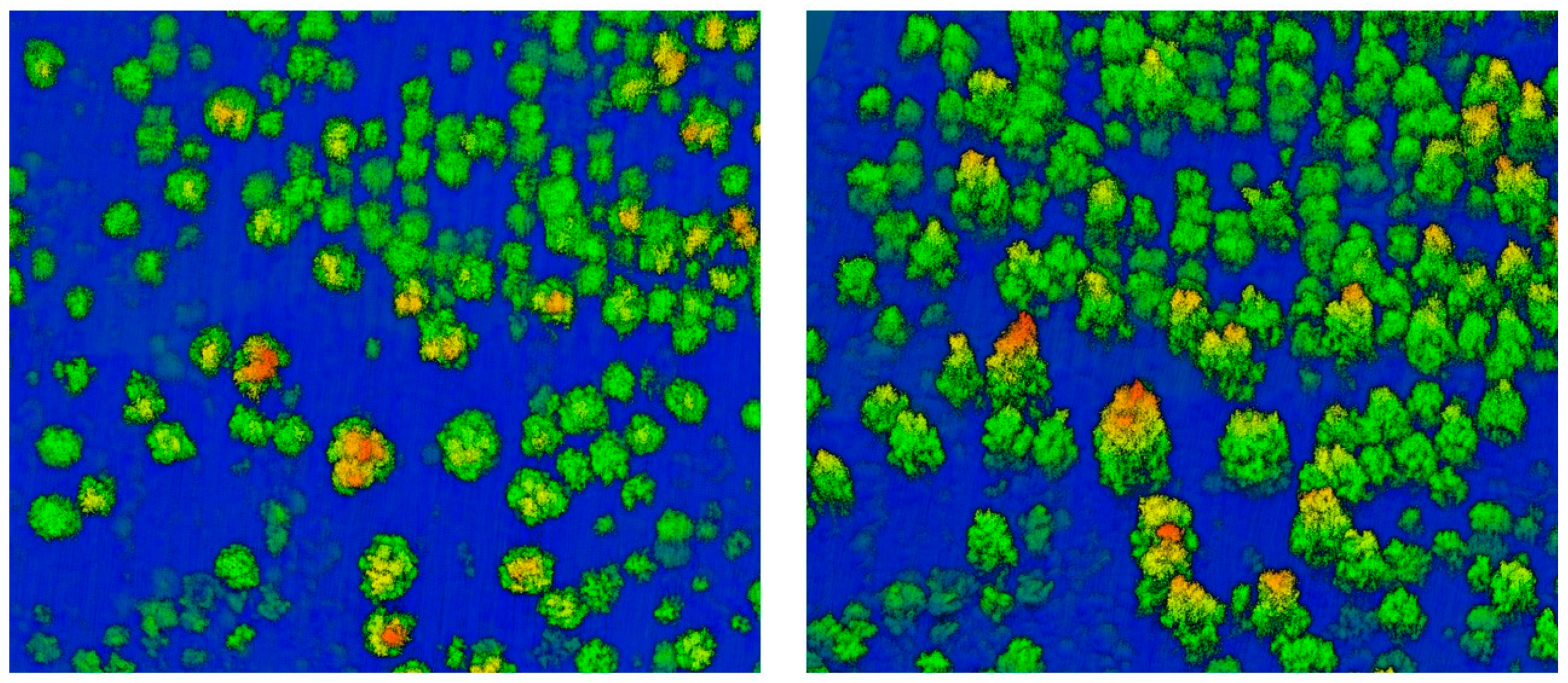
Ultra-high-density first-return LiDAR data were acquired using a Velodyne VLP-16 laser scanner (https://velodynelidar.com/vlp-16.html), mounted on a DJI Matrice 600 UAV. Flights were undertaken in January 2018 (7 years after planting) over three focal areas (total coverage = 5.8 ha) (Figure 1b). An autopiloted, cross-strip flight path flown at an altitude of 40 m above ground level at a ground speed of 3 m/s allowed a flight strip overlap of 40–50% [7,16,17], with a combined flight strip point density greater than 1000 points/m2 (Figure 2). The flight path covered six of the eight replicates of the above-mentioned treatments of the ecology trial.
Multiple, automated crown detection algorithms were employed to segment individual trees. However, the irregular crown shape of both Eucalyptus species resulted in over segmented crowns (data not shown). Thus, canopy height models (CHMs) were calculated using the Lasgrid package of LAStools (https://rapidlasso.com/lastools/lasgrid/) to manually digitize the contours of 1859 tree crowns (Figure 1c). Individual tree point clouds were then extracted from each crown using the lidR package in R [18]. Point clouds containing less than 780 points, or with a maximum 99th percentile height lower than 1.3 m (i.e., height of diameter at breast height) were removed from the analysis, leaving 1344 individual point clouds for further analysis (923 E. pauciflora, 421 E. tenuiramis). For each retained point cloud, a customized script was used to calculate 25 traits pertaining to standard descriptive traits and novel tree architectural and productivity traits (Table 1).

2.3. Statistical Analysis

All statistical analyses and data visualization were undertaken in R. Due to low survival of E. tenuiramis from the South Arm provenance, this provenance was dropped from subsequent tests. The South Arm provenance for E. pauciflora was also a significant climate outlier with high leverage and thus removed from these association analyses.

2.4. Field Validation

Field data from 557 randomly selected trees across all flown replicates of the Eucalyptus treatments were collected in May 2018 and used to validate the individual tree point clouds. Tree height (using an extendable height pole), diameter at breast height (1.3 m, DBH), cross-sectional crown width (along and perpendicular to the planting rip-line), and crown insertion height were measured for each tree. Prior to undertaking the validation analysis, slope heterogeneity among provenances within species was tested by fitting a linear model that modelled the on-ground measured trait as a function of the LiDAR-derived equivalent trait, provenance, and their interaction. Where a significant interaction was observed, the contribution of the interaction and provenance effect to the model coefficient of determination (R2) was determined by firstly removing the interaction term and then the covariate term, respectively. Linear regression models were then fitted that modelled the relationship between the ground-based trait measurement with the LiDAR-derived equivalent trait irrespective of species or provenance. Model assumptions of normality and homoscedasticity as well as overdispersion were statistically and visually assessed using simulated residuals from the fitted model using the DHARMa package, following [20]. Traits were transformed where necessary to meet model assumptions. To determine the dispersion of values around the mean, we estimated the unbiased root mean squared error (RMSE) for each trait using the following standard formula:
R M S E =   i = 1 n ( y i + y i ^ ) 2 n
where the numerator is the Pearson residual sum of squares and the denominator is the degrees of freedom of the fitted model.

3. Trait Filtering

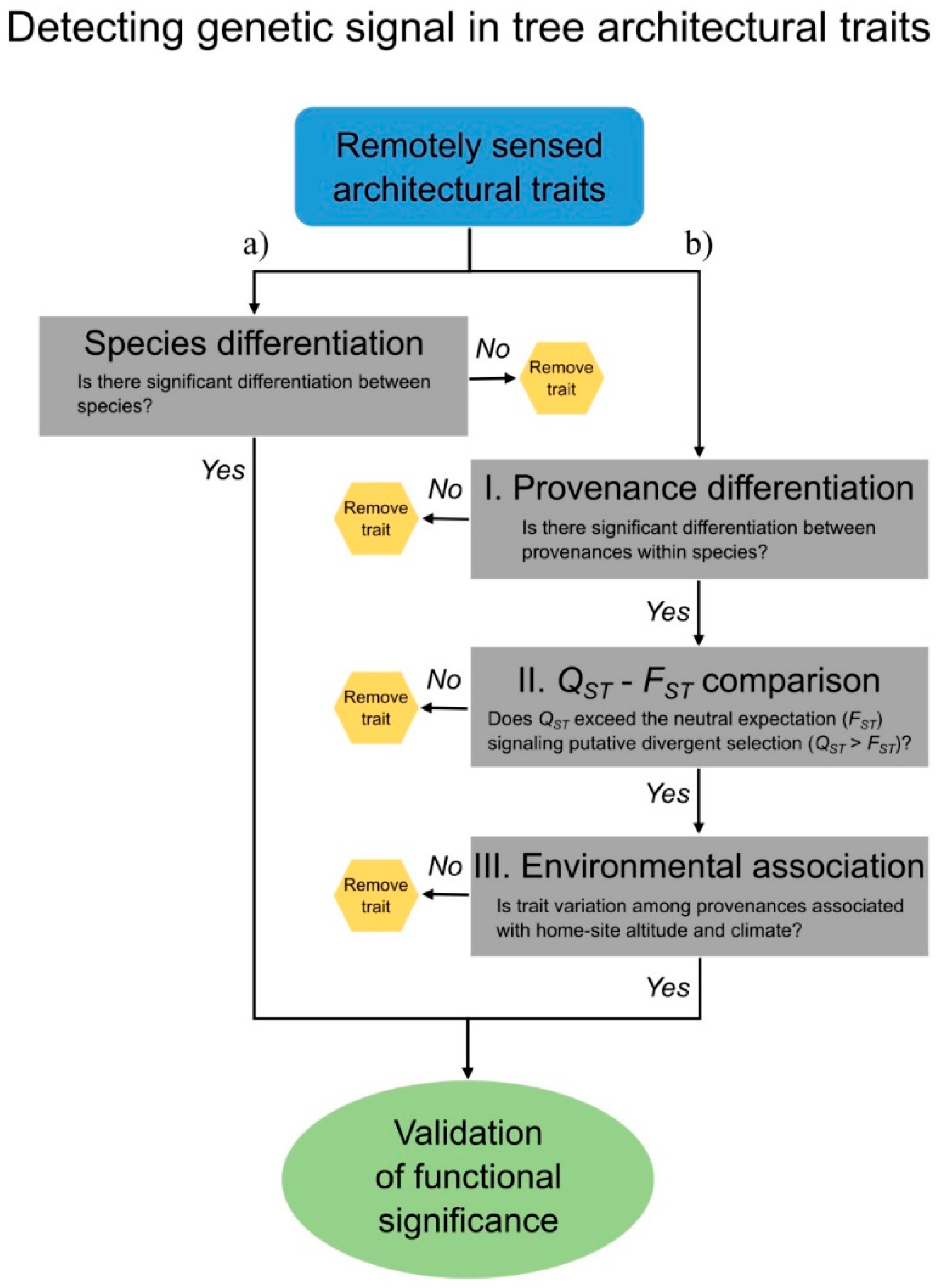
A two-phased analytical framework was developed to identify traits of biological interest. In all cases, a Bonferroni correction was applied to adjust for multiple testing using 0.05/m, where 0.05 is the significance level for rejecting the null hypothesis and m is the number of traits tested which reduced as trait filtering progressed. The first phase was to determine whether species significantly differed in their tree architecture and productivity traits (Figure 3a).
Species differences were tested using only the mixed-species treatment and fitting the following generalized mixed model using the lme4 package:
y = Xb + Zu + ε
where X is a matrix of dimensions N × p (where N is the number of observations and p is the number of predictor variables), b is a vector of complementary fixed-effect coefficients of length p, Z is the random-effects design matrix of dimensions N × q (where q is the number of random variables), u is a vector of complementary random-effect coefficients of length q, and ε is a vector of random residual terms. The terms in b comprised the overall mean and fixed species effect, while the terms in u comprised the random effect of replicate and species by replicate interaction. Model assumptions and overdispersion were visually and statistically assessed for each trait (see details in ‘Field Validation’). Fixed species effects were tested by a Type III F test, with degrees of freedom estimated following the Kenward–Roger method as implemented by the lmerTest package. When significant main fixed effects were detected, back-transformed (where needed) estimates of the least-square means and 95% confidence intervals (CI) were obtained using the emmeans package.
The second phase was undertaken at the provenance level within each species. The goal of this step was to filter tree architecture and productivity traits using three criteria to identify traits exhibiting signals of local adaptation. Firstly, traits were retained if significant provenance variation was detected (Figure 3b; Criteria I). This was achieved by fitting a univariate, individual tree mixed model (using a pedigree file) in the form of Equation (2) that fitted treatment as the fixed-effect term in b and replicate, treatment by replicate, provenance, and tree as the random-effect terms in u, where tree is the additive genetic effect for each individual. Model fitting was undertaken using the asreml package in R. The pedigree file for E. pauciflora was defined following Gauli et al. [21], accounting for a selfing rate of 10% and population inbreeding of 0.067. In the case of E. tenuiramis, a 30% selfing rate was assumed and no population inbreeding. Model assumptions of normality and homoscedasticity were visually assessed using QQ plots and plots of Pearson residuals vs. fitted values following Zurr et al. [20]. To determine whether there was significant variation among provenances for a given trait, we tested whether the provenance variance component was greater than zero using a one-tailed likelihood ratio test (LRT) with one degree of freedom. This was achieved by comparing a full and a reduced model with no provenance variance component [22]. Following Gauli et al. [21], the narrow-sense heritability for each trait was estimated using the variance components from the above described model as:
h o p 2 = σ a 2 σ a 2 + σ e 2
where σ a 2 is the estimate of the pooled additive genetic variance within populations and σ e 2 is the residual variance. Significance of the σ a 2 variance component was tested using a one-tailed LRT with one degree of freedom [22]. Variance components were also used to estimate the quantitative trait inbreeding coefficient (QST) as:
Q S T = σ p 2 σ p 2 + 2 σ a 2
where σ p 2 is the phenotypic variance component among populations and σ a 2 is defined above. The comparison of QST to the molecular analogue FST was pursued following Gauli et al. [21] using the maximum FST of 0.07 obtained for ten putatively neutral microsatellites [23]. In the case of E. tenuiramis, only the mean of ten isozymes were available for FST within northern and southern regions and thus their average FST of 0.05 was used [24]. For traits demonstrating significant provenance differentiation (Figure 3b; Criteria II), a one-tailed LRT with one degree of freedom was undertaken to test whether QST was significantly greater than FST following [25]. This involved comparing the likelihood of the unconstrained model defined above to a model where QST was constrained to FST. Traits exhibiting a significant QST > FST signaled evidence for divergent selection driving among provenance variation [26].
Additional evidence for local adaptation was pursued by testing for an association of provenance trait least-square means with home-site climate for traits exhibiting signals of divergent selection (Figure 3b; Criteria III). Least-square means were estimated by fitting the tree mixed model described above, but fitting provenance as a fixed term in b (see above). Home-site climate data were represented by minimum temperature of the coldest week (TMNCW) and maximum temperature of the warmest week (TMXWW) obtained from ANUClim V6.1 as the mean between the 1976–2005 period [27] and annual aridity (AIANN; positive value reflect increasing home-site moisture) obtained from Atlas of Living Australia (https://www.ala.org.au/). These climate variables were selected as they have been identified as potential drivers of provenance variation in functional traits [28] and species distributions in Tasmania [29]. Following Camarretta et al. [15], the least-squares means were modelled as quadratic responses to provenance home-site AIANN, TMNCW and TMXWW using linear models. Model assumption of normality and homoscedasticity of the variance were visually assessed using QQ plots and plots of Pearson residuals vs. fitted values following Zurr et al. [20]. To avoid the high collinearity among fitted polynomial terms, orthogonal linear and quadratic coefficients were fitted using the ‘poly’ function of the stats package. A two-tailed LRT with one degree of freedom was used to assess the best fit of a linear or quadratic model to the data.
Figure 3. Conceptual diagram of the two-phased analytical framework (a,b) used to filter the calculated canopy traits from the individual tree LiDAR point cloud. The first phase was to identify traits which exhibited significant differences between species. Traits which met this criterion are then validated for their functional significance. The second phase filtered traits within species using three criteria. The first criterion determined whether a trait significantly varied among the tested provenances. Traits that met this criterion were then assessed for signals of divergent selection (i.e., QST > FST; [26]). Traits signaling divergent selection were then modelled as a function of home-site environment to determine whether the variation among provenances covaried with the environment (Figure modified from Harrison [29]).
Remotesensing 12 03184 g003

4. Results

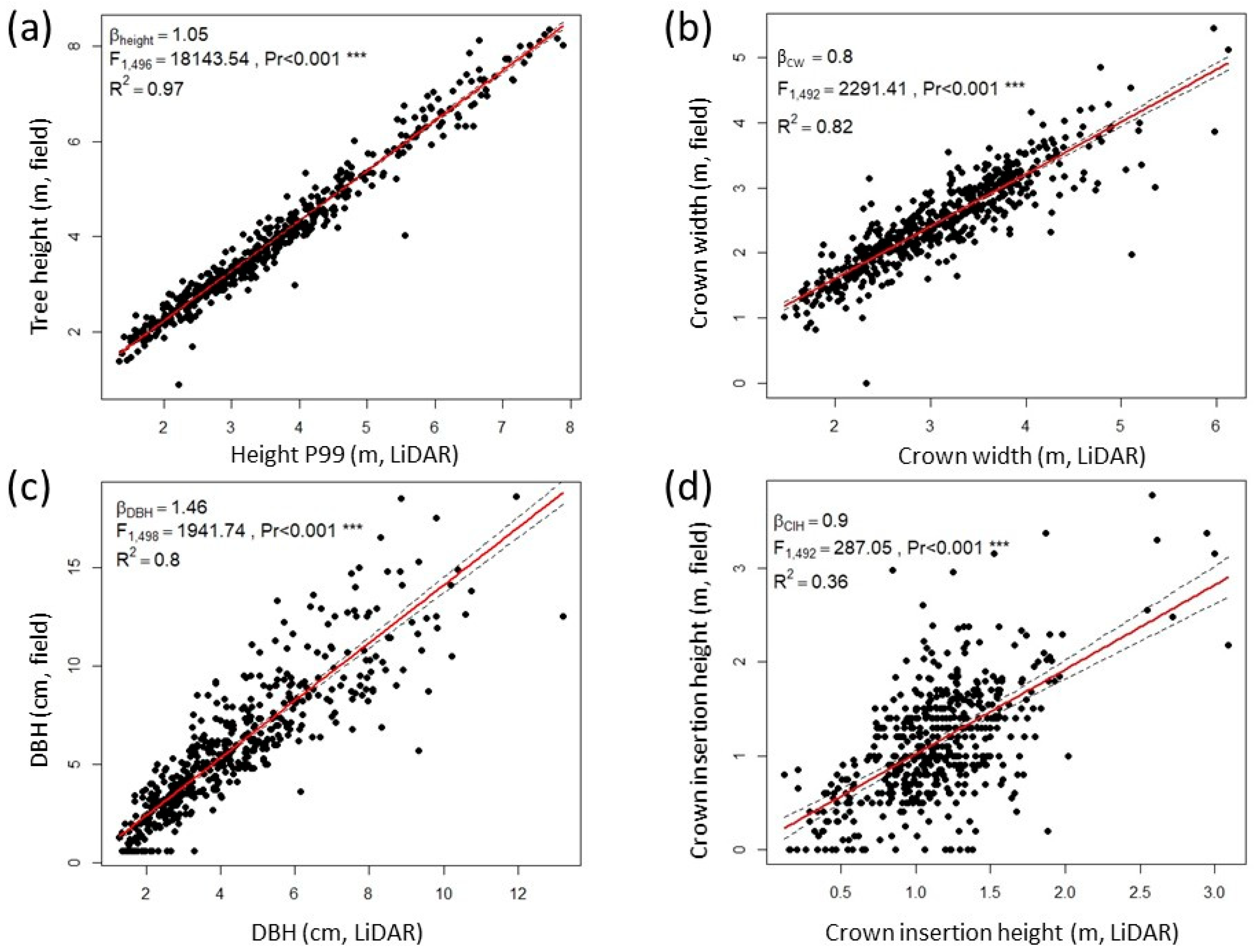
Field measurements were generally well predicted by the same measurements derived from the LiDAR point cloud, with R2 derived from linear regressions ranging between 0.80 and 0.97, with the exception of crown insertion height (R2 = 0.36) (Figure 4). Analysis of slope heterogeneity showed statistically significant (p < 0.01) interaction effects between the LiDAR-derived trait and provenance for E. pauciflora (Height P99, DBH) and E. tenuiramis (Max crown diameter). However, even when the interaction term was significant, the comparison of the change in R2 showed that the interaction term explained less than 3% of the variation explained by the covariate for E. pauciflora and less than 16% for E. tenuiramis, and thus is considered biologically unimportant compared to the main effect of the covariate. Dispersion of the LiDAR measurements around the mean as measure by RMSE ranged between 15 cm (DBH) and 49 cm (crown insertion height). The two best-predicted traits based on the relationship between the ground-based measurements and the equivalent derived traits from the individual tree point clouds had a RMSE of 25 cm (height) and 30 cm (crown width). The strong phenotypic regressions and relatively low RMSEs translated to ground and LiDAR measurements producing virtually identical patterns in species and provenance differentiation. Thirteen of the 25 derived traits significantly differed between the two focal eucalypts after a Bonferroni correction, with E. tenuiramis showing significantly higher least square means than E. pauciflora in almost all traits (Table 2). Eucalyptus tenuiramis tended to be taller, with greater above-ground biomass accumulation, and a more complex crown structure that was less dense than E. pauciflora (Table 2).
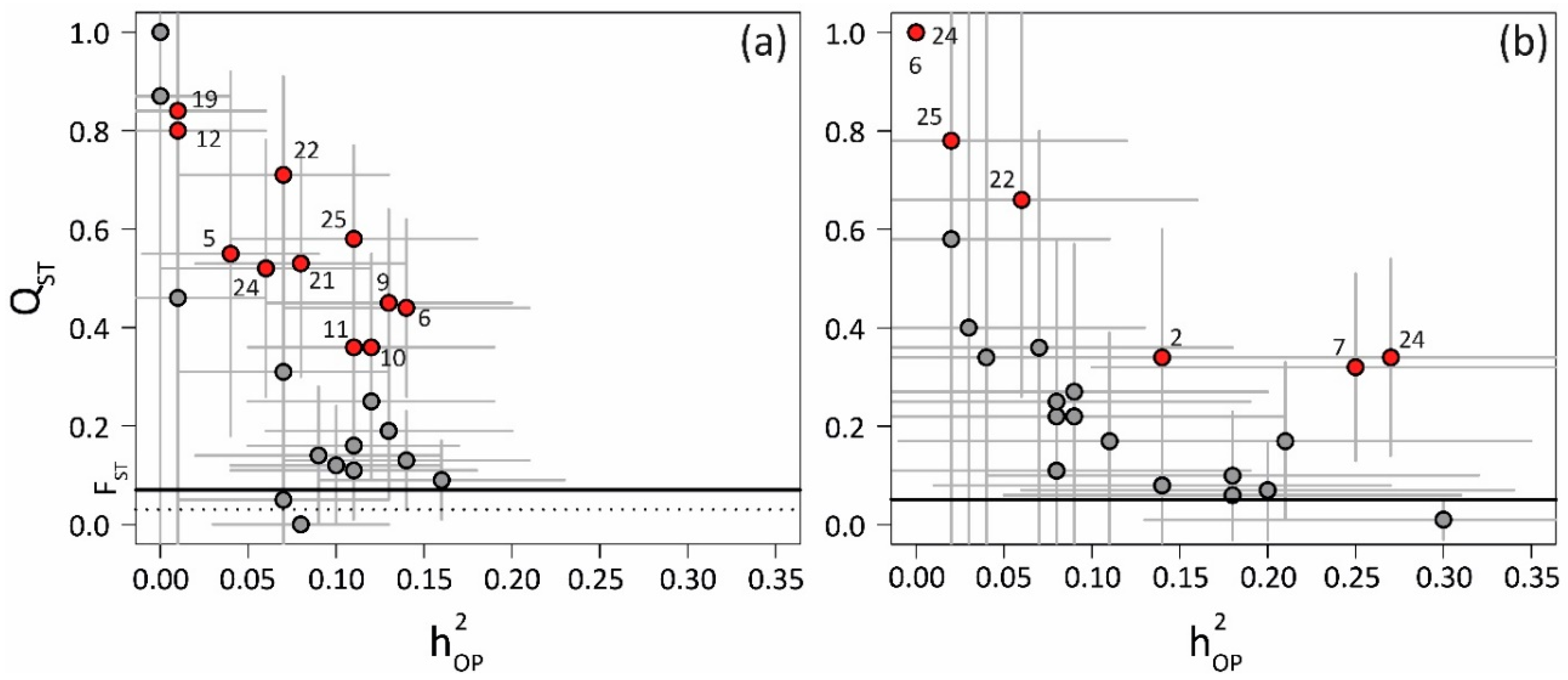
Traits significantly varied among the tested provenances, with 20 traits for E. pauciflora and ten for E. tenuiramis meeting Criteria I and retained for further analysis. Following filtering, the observed quantitative differentiation among provenances (QST) of E. pauciflora ranged between 0.09 (trait 8) and 0.84 (trait 20), and between 0.17 (trait 3) and 1.00 (traits 6 and 24) for E. tenuiramis (Figure 5; Table 3). However, only eleven and seven of these traits exhibited signals of divergent selection based on QST being significantly greater than FST for E. pauciflora and E. tenuiramis, respectively (Figure 5; Table 3). Nine and one of these traits also showed significant levels of additive genetic variation in E. pauciflora and E. tenuiramis, respectively (Table 3). In the case of E. pauciflora, home-site TMNCW and AIANN accounted for 50–77% of the variance in the eleven traits signaling divergent selection, nine of which were significant after the Bonferroni correction (Table 3). The best three models showed home-site TMNCW linearly related with increased mean height of the widest cross-section (β = 0.58, F1,7 = 17.3, P = 0.047, R2 = 71%) but decreased number of points per unit area (β = −92.7, F1,7 = 23.5, P = 0.021, R2 = 77%) and per unit volume (β = −417.2, F1,7 = 22.6, P = 0.023, R2 = 76%), the latter suggesting that provenances originating from sites with warmer winters tend to have sparser crowns. In the case of E. tenuiramis, home-site TMNCW, TMXWW, and AIANN accounted for 30–81% of the variance in the seven traits, signaling climate as a putative driver of the observed divergent selection on these traits among provenances (Table 3). Of the seven traits, only one was significantly (after Bonferroni correction) associated with a climate variable. This involved a quadratic response with TMNCW (3D:2D area; βlinear = −0.92, βquadratic = −0.64, F2,6 = 13.1, P = 0.045, R2 = 81%), suggesting that provenances originating from home sites with warmer winters tend to have less complex crown structure.

5. Discussion

Our study demonstrates the potential of UAV-LiDAR for the quantification of traditional forest traits at the individual tree-level, as well as for the development of novel LiDAR-derived traits that can offer new insights into species differentiation and local adaptation. Most of the investigated traits showed significant differences between species. Ten of these traits also showed significant provenance differences, had signals of divergent selection and co-varied with provenance home-site climate. Such variation reflects differences in tree architecture between species and provenances, which may have extended effects on the distribution of dependent organisms [30,31,32]. This is an important finding because provenances and species are increasingly being translocated across a changing landscape for the development of resilient restoration plantings [14], which may have broader community level consequences. Although structural attributes have been studied at regional scales using remote sensing [10], they have been rarely captured at a level to allow inter- and intra-specific genetic variation to be assessed [30]. While there is an increasing number of remote sensing studies quantifying individual tree-level attributes using LiDAR or photogrammetric point clouds, they mainly focus on common attributes such as tree top height, DBH and biomass [31,32,33]. Our study represents one of the first applications of remote sensing in a quantitative genetic framework for forest trees, particularly tree architectural traits. Previous applications of remote sensing in a genetic framework have studied provenance differences in heat-sum requirements when grown in a common garden environment [34], and highlighted the use of LiDAR technology for whole forest phenotyping following an area-based approach [35].
The proposed analytical framework for high-throughput phenotyping has the potential to be broadly applied to forest restoration plantings and production plantations, where pedigree information is available. The approach we describe relies on the availability of dense LiDAR data correctly segmented at the individual-tree level. In this study, individual tree delineation was carried out manually, as the complex nature of young eucalypt crowns, although clearly identifiable through visual inspection, did not provide meaningful results when implementing readily available automated crown segmentation algorithms. Many such algorithms have been proposed in the literature [36,37,38], and have been found to perform relatively well on species with regular crown shapes [39] such as conifers. As automated individual tree segmentation performed poorly and the main focus of the current study was to demonstrate an approach to rapidly phenotype and uncover genetic differences, manual digitisation was deemed sufficient. Nevertheless, further investigation into advanced machine-learning approaches [40] or methods based on modelling the 3D-shape of the tree [41] is required to resolve the individual tree segmentation of species with irregular shaped crowns.
At the species-level, our results indicate significant differentiation between the two studied eucalypt species in most tree architecture and resource allocation traits. This variation has a genetic basis as trees of the two species were alternately planted in the studied area. Surviving trees of E. tenuiramis exhibited greater growth and less dense, but more structurally complex, crowns than trees of E. pauciflora, despite the survival of E. tenuiramis being lower than E. pauciflora at this trial site [15]. While both E. pauciflora and E. tenuiramis are from the same subgenus, Eucalyptus, and often co-occur in eucalypt woodlands [42], the observed structural difference between the two species when grown in a common garden may in part reflect differences in the functional components of the ecological niche they occupy in the wild [43].
Significant genetic variation was detected at the provenance-level for many of the LiDAR-derived traits. Provenance variation is a common feature of forest tree species [13], including eucalypts, but we emphasise the novel insights now possible with LiDAR-derived traits. This is best exemplified by the negative association shown between crown point density and minimum temperature at the provenance home-site in E. pauciflora, which suggests that provenances translocated from warmer home-sites had less dense crowns at our trial site. This phenomenon could reflect an inherent genetic-based difference in growth habit of the assessed provenances or phenotypic plasticity due to trees from warmer provenances experiencing cold stress at the higher altitude trial site. Such stress would be consistent with the poorer survival reported for the lower altitude provenances at the study site [15]. Eucalypts are ever-green trees and crown density is commonly assessed as an indicator of their health, including defoliation due to pests and drought stress [44,45] and, while normally assessed on an ordered categorical scale, it has been shown to vary among provenances in field trials [46]. Indeed, these differences in crown densities are now raising new hypotheses on the extent to which they may affect the dependent communities through changes in resource use and animal feeding/nesting behaviour. Crown complexity (i.e., crown openness, vegetation layering and cover) have been linked to arthropod [47,48], bird [49,50,51] and bat species richness [52]. The introduction of non-local provenances with different crown properties, as may occur with the implementation of climate-adjusted provenancing [12], may have a broader extended effect on dependent communities. Indeed, this could potentially result in unexpected biodiversity outcomes, such as loss of habitat specialist species [53], which is opposite to the intended restoration goals. Further research is therefore needed in this area to fully untangle the intricacies between provenance translocation, crown architecture and dependent species resource utilization and behaviour.

6. Conclusions

The present study is one ofthe first to demonstrate the role of divergent selection in shaping the phenotypic variation in tree architecture and productivity traits derived using ultra-dense UAV-LiDAR point clouds. These findings advance our understanding of how the home-site climate shapes genetic variation in traits that were impractical to assess using ground-based measurements. Indeed, most noteworthy was the trend for E. pauciflora provenances originating from home-sites with warmer winters tending to have sparser crowns when translocated to the mid-altitude field trial site. Species are being increasingly translocated across and outside their native distribution to mitigate biodiversity loss due to increasing maladaptation as climate changes. The present study highlights the need to consider whether translocated provenances with different crown architecture and productivity traits impact the habitat requirements of the biotic communities at the recipient site. Utilising rapid technological advances in UAV platform and sensor development together with data fusion approaches (e.g. UAV-LiDAR and hyperspectral imaging) will provide new understandings on the genetic diversity and functional value of the identified tree architecture and productivity traits to better guide the management of natural resources during an era of rapid change.

Supplementary Materials

The following are available online at https://www.mdpi.com/2072-4292/12/19/3184/s1, Table S1. Longitude and latitude (in decimal degrees), altitude above sea level (m a.s.l.), mean annual aridity index (AIANN), minimum temperature of the coldest week (TMNCW) and maximum temperature of the warmest week (TMXWW) for each provenance sampled for both focal eucalypt species, as well as trial site (last row).

Author Contributions

Conceptualization, N.C.; Methodology, N.C., P.A.H. and B.M.P.; Software, P.A.H., N.C. and B.M.P.; Validation, N.C., B.M.P. and P.A.H.; Formal Analysis, N.C., P.A.H. and B.M.P.; Investigation, N.C., B.M.P. and P.A.H.; Resources, A.L. and M.H.; Data Curation, N.C., A.L. and P.A.H.; Writing—Original Draft Preparation, N.C.; Writing—Review & Editing, P.A.H., M.H., A.L., B.M.P., N.D.; Visualization, N.C.; Supervision, P.A.H., B.M.P., A.L., and M.H.; Project Administration, N.C.; Funding Acquisition, M.H. and B.M.P. All authors have read and agreed to the published version of the manuscript.

Funding

Trial establishment was supported by a Tasmanian State Government grant to offset government carbon emissions (offered to Greening Australia by then Premier Jim Bacon) as well as an Australian Research Council (ARC) Linkage Grant (LP0991026) held in partnership with Greening Australia. The ARC Industrial Transformation Training Centre for Forest Value (IC150100004) provided further support including a PhD scholarship for NC.

Acknowledgments

We thank Woodlea Nursery for plant production, Tanya Bailey, Paul Tilyard and Dalila Pasquini for their assistance with field work, Darren Turner for drone operations.

Conflicts of Interest

The authors declare no conflict of interests.

References

  1. Kellner, J.R.; Albert, L.P.; Burley, J.T.; Cushman, K.C. The case for remote sensing of individual plants. Am. J. Bot. 2019, 106, 1139–1142. [Google Scholar] [CrossRef] [PubMed] [Green Version]
  2. Krause, S.; Sanders, T.G.M.; Mund, J.P.; Greve, K. UAV-based photogrammetric tree height measurement for intensive forest monitoring. Remote Sens. 2019, 11, 758. [Google Scholar] [CrossRef] [Green Version]
  3. Alberto, F.J.; Aitken, S.N.; Alía, R.; González-Martínez, S.C.; Hänninen, H.; Kremer, A.; Lefèvre, F.; Lenormand, T.; Yeaman, S.; Whetten, R.; et al. Potential for evolutionary responses to climate change - evidence from tree populations. Glob. Chang. Biol. 2013, 19, 1645–1661. [Google Scholar] [CrossRef] [PubMed] [Green Version]
  4. Dungey, H.S.; Dash, J.P.; Pont, D.; Clinton, P.W.; Watt, M.S.; Telfer, E.J. Phenotyping whole forests will help to track genetic performance. Trends Plant Sci. 2018, 23, 854–864. [Google Scholar] [CrossRef] [PubMed]
  5. Fankhauser, K.E.; Strigul, N.S.; Gatziolis, D. Augmentation of traditional forest inventory and Airborne laser scanning with unmanned aerial systems and photogrammetry for forest monitoring. Remote Sens. 2018, 10, 1562. [Google Scholar] [CrossRef] [Green Version]
  6. Solvin, T.M.; Puliti, S.; Steffenrem, A. Use of UAV photogrammetric data in forest genetic trials: Measuring tree height, growth, and phenology in Norway spruce (Picea abies L. Karst.). Scand. J. For. Res. 2020, 1–12. [Google Scholar] [CrossRef]
  7. Wallace, L.; Musk, R.; Lucieer, A. An assessment of the repeatability of automatic forest inventory metrics derived from UAV-borne laser scanning data. IEEE Trans. Geosci. Remote Sens. 2014, 52, 7160–7169. [Google Scholar] [CrossRef]
  8. Grubinger, S.; Coops, N.C.; Stoehr, M.; El-Kassaby, Y.A.; Lucieer, A.; Turner, D. Modeling realized gains in Douglas-fir (Pseudotsuga menziesii) using laser scanning data from unmanned aircraft systems (UAS). For. Ecol. Manage. 2020, 473, 118284. [Google Scholar] [CrossRef]
  9. du Toit, F.; Coops, N.C.; Tompalski, P.; Goodbody, T.R.H.; El-Kassaby, Y.A.; Stoehr, M.; Turner, D.; Lucieer, A. Characterizing variations in growth characteristics between Douglas-fir with different genetic gain levels using airborne laser scanning. Trees-Struct. Funct. 2020, 34, 649–664. [Google Scholar] [CrossRef]
  10. Camarretta, N.; Harrison, P.A.; Bailey, T.; Potts, B.; Lucieer, A.; Davidson, N.; Hunt, M. Monitoring forest structure to guide adaptive management of forest restoration: A review of remote sensing approaches. New For. 2019, 1–24. [Google Scholar] [CrossRef]
  11. Breed, M.F.; Harrison, P.A.; Bischoff, A.; Durruty, P.; Gellie, N.J.C.C.; Gonzales, E.K.; Havens, K.; Karmann, M.; Kilkenny, F.F.; Krauss, S.L.; et al. Priority actions to improve provenance decision-making. Bioscience 2018, 68, 510–516. [Google Scholar] [CrossRef]
  12. Prober, S.M.; Byrne, M.; McLean, E.H.; Steane, D.A.; Potts, B.M.; Vaillancourt, R.E.; Stock, W.D. Climate-adjusted provenancing: A strategy for climate-resilient ecological restoration. Front. Ecol. Evol. 2015, 3, 40–53. [Google Scholar] [CrossRef] [Green Version]
  13. White, T.L.; Adams, W.; Neale, D. Forest Genetics; CABI: Wallingford, UK, 2007. [Google Scholar]
  14. Aitken, S.N.; Bemmels, J.B. Time to get moving: Assisted gene flow of forest trees. Evol. Appl. 2016, 9, 271–290. [Google Scholar] [CrossRef] [PubMed]
  15. Camarretta, N.; Harrison, P.A.; Bailey, T.; Davidson, N.; Lucieer, A.; Hunt, M.; Potts, B.M. Stability of species and provenance performance when translocated into different community assemblages. Restor. Ecol. 2020, 28, 447–458. [Google Scholar] [CrossRef]
  16. Wallace, L.; Lucieer, A.; Turner, D.; Watson, C. Error assessment and mitigation for hyper-temporal UAV-borne LiDAR surveys of forest inventory. In Proceedings of the SilviLaser 2011, Hobart, Australia, 16–20 October 2011; pp. 1–14. [Google Scholar]
  17. Stone, C.; Caccamo, G.; Osborn, J.; Lucieer, A.; Iqbal, I.; McCoull, C.; Harwin, S.; Turner, D.; Pishchugin, A.; Gautam, D.; et al. Optimising Remotely Acquired, Dense Point Cloud Data for Plantation Inventory; Forest and Wood Products Australia: Melbourne, VIC, Australia, 2018; Volume 61.
  18. R Core Team R: A Language and Environment for Statistical Computing. Available online: https://www.r-project.org (accessed on 9 January 2017).
  19. Jucker, T.; Caspersen, J.; Chave, J.; Antin, C.; Barbier, N.; Bongers, F.; Dalponte, M.; van Ewijk, K.Y.; Forrester, D.I.; Haeni, M.; et al. Allometric equations for integrating remote sensing imagery into forest monitoring programmes. Glob. Chang. Biol. 2017, 23, 177–190. [Google Scholar] [CrossRef] [PubMed]
  20. Zuur, A.F.; Ieno, E.N. A protocol for conducting and presenting results of regression-type analyses. Methods Ecol. Evol. 2016, 7, 636–645. [Google Scholar] [CrossRef]
  21. Gauli, A.; Vaillancourt, R.E.; Bailey, T.G.; Steane, D.A.; Potts, B.M. Evidence for local climate adaptation in early-life traits of Tasmanian populations of Eucalyptus pauciflora. Tree Genet. Genomes 2015, 11, 14. [Google Scholar] [CrossRef]
  22. Gilmour, A.R.; Gogel, B.J.; Cullis, B.R.; Thompson, R. ASReml User Guide Release 3.0; VSN International Ltd.: Hemel Hempstead, UK, 2009. [Google Scholar]
  23. Gauli, A.; Steane, D.A.; Vaillancourt, R.E.; Potts, B.M. Molecular genetic diversity and population structure in Eucalyptus pauciflora subsp. pauciflora (Myrtaceae) on the island of Tasmania. Aust. J. Bot. 2014, 62, 175–188. [Google Scholar] [CrossRef]
  24. Turner, C.; Wiltshire, R.J.E.; Potts, B.M.; Vaillancourt, R.E. Allozyme variation and conservation of the Tasmanian endemics, Eucalyptus risdonii, E. Tenuiramis and E. coccifera. Conserv. Genet. 2000, 1, 209–216. [Google Scholar] [CrossRef]
  25. Dutkowski, G.W.; Potts, B.M. Genetic variation in the susceptibility of Eucalyptus globulus to drought damage. Tree Genet. Genomes 2012, 8, 757–773. [Google Scholar] [CrossRef]
  26. Leinonen, T.; McCairns, R.J.S.; O’Hara, R.B.; Merilä, J. QST–FST comparisons: Evolutionary and ecological insights from genomic heterogeneity. Nat. Rev. Genet. 2013, 14, 179–190. [Google Scholar] [CrossRef]
  27. Xu, T.; Hutchinson, M.F. New developments and applications in the ANUCLIM spatial climatic and bioclimatic modelling package. Environ. Model. Softw. 2013, 40, 267–279. [Google Scholar] [CrossRef]
  28. Prober, S.M.; Potts, B.M.; Bailey, T.; Byrne, M.; Dillon, S.; Harrison, P.A.; Hoffmann, A.A.; Jordan, R.; Mclean, E.H.; Steane, D.A.; et al. Climate adaptation and ecological restoration in eucalypts. Proc. R. Soc. Victoria 2016, 128, 40–53. [Google Scholar] [CrossRef] [Green Version]
  29. Harrison, P.A. Integrating Climate Change into Conservation and Restoration Strategies: The Case of the Tasmanian Eucalypts. Ph.D. Thesis, University of Tasmania, Hobart, Australia, 2017. [Google Scholar]
  30. Santini, F.; Kefauver, S.C.; Resco de Dios, V.; Araus, J.L.; Voltas, J. Using unmanned aerial vehicle-based multispectral, RGB and thermal imagery for phenotyping of forest genetic trials: A case study in Pinus halepensis. Ann. Appl. Biol. 2019, 174, 262–276. [Google Scholar] [CrossRef] [Green Version]
  31. Dalponte, M.; Frizzera, L.; Gianelle, D. How to map forest structure from aircraft, one tree at a time. Ecol. Evol. 2018, 8, 5611–5618. [Google Scholar] [CrossRef] [PubMed]
  32. Burt, A.; Disney, M.; Calders, K. Extracting individual trees from lidar point clouds using treeseg. Methods Ecol. Evol. 2019, 10, 438–445. [Google Scholar] [CrossRef] [Green Version]
  33. Duncanson, L.; Dubayah, R. Monitoring individual tree-based change with airborne lidar. Ecol. Evol. 2018, 8, 5079–5089. [Google Scholar] [CrossRef]
  34. Li, H.; Wang, X.; Hamann, A. Genetic adaptation of aspen ( Populus tremuloides ) populations to spring risk environments: A novel remote sensing approach. Can. J. For. Res. 2010, 40, 2082–2090. [Google Scholar] [CrossRef]
  35. Bombrun, M.; Dash, J.P.; Pont, D.; Watt, M.S.; Pearse, G.D.; Dungey, H.S. Forest-Scale Phenotyping: Productivity Characterisation Through Machine Learning. Front. Plant Sci. 2020, 11, 1–14. [Google Scholar] [CrossRef]
  36. Kattenborn, T.; Sperlich, M.; Bataua, K.; Koch, B. Automatic Single Tree Detection in Plantations using UAV-based Photogrammetric Point clouds. ISPRS—Int. Arch. Photogramm. Remote Sens. Spat. Inf. Sci. 2014, XL-3, 139–144. [Google Scholar] [CrossRef] [Green Version]
  37. Eysn, L.; Hollaus, M.; Lindberg, E.; Berger, F.; Monnet, J.M.; Dalponte, M.; Kobal, M.; Pellegrini, M.; Lingua, E.; Mongus, D.; et al. A benchmark of lidar-based single tree detection methods using heterogeneous forest data from the Alpine Space. Forests 2015, 6, 1721–1747. [Google Scholar] [CrossRef] [Green Version]
  38. Nevalainen, O.; Honkavaara, E.; Tuominen, S.; Viljanen, N.; Hakala, T.; Yu, X.; Hyyppä, J.; Saari, H.; Pölönen, I.; Imai, N.; et al. Individual tree detection and classification with UAV-based photogrammetric point clouds and hyperspectral imaging. Remote Sens. 2017, 9, 185. [Google Scholar] [CrossRef] [Green Version]
  39. Mohan, M.; Silva, C.; Klauberg, C.; Jat, P.; Catts, G.; Cardil, A.; Hudak, A.; Dia, M. Individual Tree Detection from Unmanned Aerial Vehicle (UAV) Derived Canopy Height Model in an Open Canopy Mixed Conifer Forest. Forests 2017, 8, 340. [Google Scholar] [CrossRef] [Green Version]
  40. Weinstein, B.G.; Marconi, S.; Bohlman, S.; Zare, A.; White, E. Individual tree-crown detection in rgb imagery using semi-supervised deep learning neural networks. Remote Sens. 2019, 11, 1309. [Google Scholar] [CrossRef] [Green Version]
  41. Balsi, M.; Esposito, S.; Fallavollita, P.; Nardinocchi, C. Single-tree detection in high-density LiDAR data from UAV-based survey. Eur. J. Remote Sens. 2018, 51, 679–692. [Google Scholar] [CrossRef] [Green Version]
  42. Williams, K.J.; Potts, B.M. The natural distribution of Eucalyptus species in Tasmania. Tasforests 1996, 8, 39–149. [Google Scholar]
  43. Schellenberger Costa, D.; Gerschlauer, F.; Kiese, R.; Fischer, M.; Kleyer, M.; Hemp, A. Plant niche breadths along environmental gradients and their relationship to plant functional traits. Divers. Distrib. 2018, 24, 1869–1882. [Google Scholar] [CrossRef] [Green Version]
  44. Barry, K.M.; Stone, C.; Mohammed, C.L. Crown-scale evaluation of spectral indices for defoliated and discoloured eucalypts. Int. J. Remote Sens. 2008, 29, 47–69. [Google Scholar] [CrossRef] [Green Version]
  45. Moore, T.L.; Ruthrof, K.X.; Craig, M.D.; Valentine, L.E.; Hardy, G.E.S.J.; Fleming, P.A. Living (and reproducing) on the edge: Reproductive phenology is impacted by rainfall and canopy decline in a Mediterranean eucalypt. Aust. J. Bot. 2016, 64, 129–141. [Google Scholar] [CrossRef]
  46. Low, C.B.; Shelbourne, C.J.A. Performance of Eucalyptus globulus, E. maidenii, E. nitens, and other eucalypts in Northland and Hawke’s Bay at ages 7 and 11 years. New Zeal. J. For. Sci. 1999, 29, 274–288. [Google Scholar]
  47. Müller, J.; Bae, S.; Röder, J.; Chao, A.; Didham, R.K. Airborne LiDAR reveals context dependence in the effects of canopy architecture on arthropod diversity. For. Ecol. Manage. 2014, 312, 129–137. [Google Scholar] [CrossRef]
  48. Setiawan, N.N.; Vanhellemont, M.; Baeten, L.; Gobin, R.; De Smedt, P.; Proesmans, W.; Ampoorter, E.; Verheyen, K. Does neighbourhood tree diversity affect the crown arthropod community in saplings? Biodivers. Conserv. 2016, 25, 169–185. [Google Scholar] [CrossRef]
  49. Müller, J.; Stadler, J.; Brandl, R. Composition versus physiognomy of vegetation as predictors of bird assemblages: The role of lidar. Remote Sens. Environ. 2010, 114, 490–495. [Google Scholar] [CrossRef]
  50. Munro, N.T.; Fischer, J.; Barrett, G.; Wood, J.; Leavesley, A.; Lindenmayer, D.B. Bird’s response to revegetation of different structure and floristics-Are ‘restoration plantings’ restoring bird communities? Restor. Ecol. 2011, 19, 223–235. [Google Scholar] [CrossRef]
  51. North, M.P.; Kane, J.T.; Kane, V.R.; Asner, G.P.; Berigan, W.; Churchill, D.J.; Conway, S.; Gutiérrez, R.J.; Jeronimo, S.; Keane, J.; et al. Cover of tall trees best predicts California spotted owl habitat. For. Ecol. Manag. 2017, 405, 166–178. [Google Scholar] [CrossRef]
  52. Froidevaux, J.S.P.; Zellweger, F.; Bollmann, K.; Jones, G.; Obrist, M.K. From field surveys to LiDAR: Shining a light on how bats respond to forest structure. Remote Sens. Environ. 2016, 175, 242–250. [Google Scholar] [CrossRef] [Green Version]
  53. Hanzelka, J.; Reif, J. Effects of vegetation structure on the diversity of breeding bird communities in forest stands of non-native black pine (Pinus nigra A.) and black locust (Robinia pseudoacacia L.) in the Czech Republic. For. Ecol. Manag. 2016, 379, 102–113. [Google Scholar] [CrossRef]
Figure 1. Location of the restoration common-garden restoration trial site at Dungrove (black dot) relative to the Midlands biodiversity hotspot (grey surface) of the south-east island of Tasmania, Australia (Panel (a)). Panel b shows the layout of the various experiments established at the trail site, including the ecology trials represented by the yellow blocks. Also shown in Panel (b) are the three targeted areas flown using UAV-LiDAR represented by the red boxes. Panel (c) corresponds to the three canopy height models (CHMs) derived from the UAV-LiDAR point clouds. Heights are represented by a color gradient, where blue corresponds to ground-level returns and red corresponds the tallest canopies across the flight area. The coordinate system used for the maps is EPSG 28,355–GDA94/MGA zone 55S.
Remotesensing 12 03184 g001
Figure 2. Example scenes of the LiDAR point cloud collected over the study site, colored by elevation (blue to red = 0–10 m). The left panel shows the bird’s eye view, while the right panel shows the isometric view.
Remotesensing 12 03184 g002
Figure 4. Relationship between field-measured and LiDAR-derived tree height (a), crown width (b), stem DBH (c) and crown insertion height (d). Points correspond to the 557 trees sampled in the field, with the line of best fit (red line) and 95% confidence intervals (dashed black lines) shown. Within each plot, the slope (β), F statistic with its numerator and denominator degrees of freedom and corresponding p-value and the coefficient of determination (R2) are shown.
Remotesensing 12 03184 g004
Figure 5. Quantitative inbreeding coefficient (QST) and narrow-sense heritability ( h O P 2 ) estimates (with standard errors; grey lines) for traits reported in the present study for Eucalyptus pauciflora (a) and E. tenuiramis (b). The solid horizontal line indicates the maximum FST (both Eucalyptus species) based on putatively neutral molecular markers (E. pauciflora—microsatellite; E. tenuiramis—isozymes) and the dotted line indicates the mean FST of any microsatellite locus (E. pauciflora only). Symbols colored in red correspond to traits that exhibited significant signals of divergent selection (QST > FST) after filtering traits for significant provenance variation (see Figure 3). Numbers next to symbols correspond to the trait numbers in Table 1.
Remotesensing 12 03184 g005
Table 1. Description of the 25 derived traits from the individual tree-level LiDAR point clouds. The unit of measurement for eachderived trait is shown after the trait name.
TraitsDescription of LiDAR-derived traits
1–Number of pointsNumber of points within individual point cloud.
2–Height skewnessSkewness of the distribution of heights of each point cloud.
3–Height CVCoefficient of variation of heights from each point cloud.
4–Quantile coefficient of dispersionA measure of dispersion of the height measurements comparable between trees and across studies. Calculated as Q3 − Q1/Q3 + Q1.
5–Height mode (m)Mode of height within the point cloud.
6–Height median (m)Median of height within the point cloud.
7–Height P50 (m)50th percentile of height within point cloud.
8–Height P75 (m)75th percentile of height within point cloud.
9–Height P99 (m)99th percentile of height within point cloud.
10–DBH (cm)Diameter at 1.3 m, derived from a general allometric equation using total tree height and maximum Euclidean crown width [19].
11–Above-ground biomass (AGB - kg)AGB estimated through the allometric equation developed by Jucker et al. [19], using height P99 and max crown diameter. Measured as dry weight.
12–Crown insertion height (m)Mean height from the ground to the base of the crown.
13–Max crown diameter (m)The widest cross-section of the crown in any given direction.
14–Crown surface area (m2)The surface area of a 3D convex hull calculated using the point cloud defined above the canopy insertion point.
15–Crown projected area (m2)The area of the projected polygon (shapefile) describing the crown ground cover.
16–Crown volume (convex hull)Crown volume of a 3D convex hull calculated from the point cloud defined above crown insertion. It is calculated using the ‘convhulln’ function of the R geometry package.
17–Height to area ratio (m/m2)The ratio of crown height to crown area. It represents the crown height per unit of area.
18–Height to volume ratio (m/m3)The ratio of crown height to crown volume. It represents the crown height per unit of volume
19–Height of widest cross-section (m)Height of the crown at its widest cross-section.
20–Mean height to height of widest cross-section ratioRatio between mean tree height and the height of its widest cross-section.
21–Points to area ratio (points/m2)The ratio of the number of points to crown area, representing a measure of crown density.
22–Points to volume ratio (points/m3)The ratio of the number of points to crown volume, representing a measure of crown density.
23–Crown skewnessSkewness of the height distribution within each tree (median − Q1)/(Q3 − median).
24–Area (3D:2D)The ratio between crown volume calculated from the point cloud (i.e., convex hull) and the crown area obtained from the shapefile.
25–Rumple indexCalculated as the ratio between crown surface area and ground-projected surface area, this index reflects crown structural complexity. Calculated using the “rumple_index” function from the lidR package.
Table 2. Statistical results from the species-level linear mixed-effect model for 25 traits derived from individual tree LiDAR point clouds. Shown is the estimated numerator (Num) and denominator (Den) degrees of freedom based on the Kenward–Roger approximation, the F statistic, and its probability for the fixed-effect difference between E. pauciflora and E. tenuiramis. Also shown are the least-square means for each trait estimated from the fitted mixed-effects model. Values in bold correspond to traits significant after a Bonferroni adjustment.
TraitLeast-Square MeanDegrees of FreedomFP
E. paucifloraE. tenuiramisNumDen
15035843414.917.30.009
2−0.76−0.6115.88.00.032
30.330.3515.010.00.025
40.210.2415.112.70.016
52.183.2915.022.30.005
62.293.3615.049.50.001
70.510.9515.025.30.004
82.103.3315.046.30.001
93.144.7814.963.50.001
103.585.8214.890.30.000
111.916.4014.971.00.000
121.051.3115.019.80.007
132.903.5014.854.60.001
1416.5030.7014.963.90.001
155.157.3914.943.80.001
165.7514.1714.957.50.001
170.220.1814.725.00.005
180.710.4314.739.30.002
191.632.1514.735.20.002
202.162.4615.38.60.031
2126423514.67.30.047
2281554014.669.20.001
231.331.3014.90.20.704
243.304.2514.936.60.002
253.895.0114.876.10.000
Table 3. Genetic parameters for the 25 traits derived from individual tree LiDAR point clouds. Shown for each species is the provenance one-tailed Chi-squared statistic and its significance from zero, the quantitative inbreeding coefficient (QST ± standard errors) and narrow-sense heritability ( h O P 2 ± standard errors) estimates, and the QST > FST one-tail Chi-squared statistic and its significance. Environmental association modelling of provenance least-square means for traits signalling divergent selection (QST > FST) as a function of altitude or climate showing the sign of the relationship, the best environmental predictor, the coefficient of determination expressed as a percentage, and the significance of the association. In all cases, the best environmental association models had a linear slope except for trait 24 that had a quadratic slope. Values in bold correspond to traits significant after a Bonferroni adjustment.
TraitEucalyptus Pauciflora Eucalyptus Tenuiramis
ProvenanceGenetic ParametersQST > FSTEnvironmental AssociationProvenanceGenetic ParametersQST > FSTEnvironmental Association
χ 1 2 QST h O P 2 χ 1 2 χ 1 2 Qst h O P 2 χ 1 2
10.4 ns0.00 ± 0.000.08 ± 0.05 6.9 **0.08 ± 0.120.14 ± 0.13
231.0 ***0.31 ± 0.230.07 ± 0.067.7 ** 29.7 ***0.34 ± 0.260.14 ± 0.127.2 **(+) TMNCW 50% *
36.0 **0.87 ± 3.160.00 ± 0.04 12.0 ***0.36 ± 0.440.07 ± 0.115 *
412.8 ***0.11 ± 0.100.11 ± 0.070.5 ns 15.7 ***0.17 ± 0.160.21 ± 0.143.1 *
548.2 ***0.55 ± 0.370.04 ± 0.0515.5 ***(+) TMNCW 50% *1.9 ns0.34 ± 0.720.04 ± 0.11
6136.4 ***0.44 ± 0.180.14 ± 0.0717.0 ***(+) TMNCW 62% *22.6 ***1.00 ± 0.000.00 ± 0.0014.3 ***(−) TMNCW 64% *
723.3 ***0.13 ± 0.100.14 ± 0.071.9 ns 82.2 ***0.32 ± 0.190.25 ± 0.157.6 **(+) AIANN 44% ns
817.0 ***0.09 ± 0.080.16 ± 0.070.3 ns 1.7 ns0.11 ± 0.200.08 ± 0.11
9134.3 ***0.45 ± 0.190.13 ± 0.0717.7 ***(−) AIANN 63% *6.9 **0.58 ± 1.170.02 ± 0.09
1081.3 ***0.36 ± 0.190.12 ± 0.0712.9 ***(−) AIANN 63% *10.1 **0.27 ± 0.300.09 ± 0.114.4 *
1170.4 ***0.36 ± 0.190.11 ± 0.0612.3 ***(−) AIANN 54% *7.1 **0.17 ± 0.220.11 ± 0.12
1266.3 ***0.80 ± 0.530.01 ± 0.0520.6 ***(+) TMNCW 69% **5.3 *1.00 ± 0.000.00 ± 0.00
1320.5 ***0.16 ± 0.130.11 ± 0.062.3 ns 5.8 **0.07 ± 0.100.20 ± 0.14
1445.3 ***0.25 ± 0.160.12 ± 0.077.4 ** 6.4 **0.25 ± 0.330.08 ± 0.11
1512.3 ***0.12 ± 0.120.10 ± 0.060.9 ns 4.5 *0.06 ± 0.090.18 ± 0.13
1633.5 ***0.19 ± 0.140.13 ± 0.074.5 * 0.5 ns1.00 ± 0.000.00 ± 0.00
172.6 ns0.05 ± 0.100.07 ± 0.06 4.8 *0.22 ± 0.290.09 ± 0.12
1811.1 ***0.14 ± 0.140.09 ± 0.071.2 ns 5.4 *0.40 ± 0.780.03 ± 0.10
1973.8 ***0.84 ± 0.520.01 ± 0.0522.7 ***(+) TMNCW 71% **7.3 **0.10 ± 0.130.18 ± 0.14
204.5 *1.00 ± 0.000.00 ± 0.00 3.5 *0.01 ± 0.040.30 ± 0.17
21109.7 ***0.53 ± 0.230.08 ± 0.0619.9 ***(−) TMNCW 77% **83.0 ***0.34 ± 0.200.27 ± 0.167.2 **(−) TMXWW 67% *
22203.0 ***0.71 ± 0.200.07 ± 0.0629.4 ***(−) TMNCW 76% **65.9 ***0.66 ± 0.400.06 ± 0.1014.6 ***(+) TMNCW 56% ns
234.4 *0.46 ± 1.130.01 ± 0.05 6.2 **0.22 ± 0.310.08 ± 0.11
2484.5 ***0.52 ± 0.260.06 ± 0.0617.4 ***(−) AIANN 62% *10.3 **1.00 ± 0.000.00 ± 0.009.6 **(−) TMNCW 81% **
25182.9 ***0.58 ± 0.190.11 ± 0.0723.7 ***(−) AIANN 64% **32.7 ***0.78 ± 0.910.02 ± 0.1010.6 **(−) TMNCW 30% ns
Climate variables: AIANN = mean annual aridity index; TMNCW = minimum temperature of the coldest week; TMXWW = maximum temperature of the warmest week. Significance levels: *** = p < 0.001, ** = p < 0.01, * = p < 0.05, ns = p > 0.05.