Article

GPS/BDS RTK Positioning Based on Equivalence Principle Using Multiple Reference Stations

Institute of Space Science, Shandong University, Weihai 264209, China
*
Author to whom correspondence should be addressed.
Remote Sens. 2020, 12(19), 3178; https://doi.org/10.3390/rs12193178
Submission received: 23 July 2020 / Revised: 12 September 2020 / Accepted: 27 September 2020 / Published: 28 September 2020

Abstract

:
Reliable real-time kinematic (RTK) is crucially important for emerging global navigation satellite systems (GNSSs) applications, such as drones and unmanned vehicles. The performance of conventional single baseline RTK (SBRTK) with one reference station degrades greatly in dense, urban environments, due to signal blockage and multipath error. The increasing use of multiple reference stations for kinematic positioning can improve RTK positioning accuracy and availability in urban areas. This paper proposes a new algorithm for multi-baseline RTK (MBRTK) positioning based on the equivalence principle. The advantages of the solution are to keep observation independent and increase the redundancy to estimate the unknown parameters. The equivalent double-differenced (DD) observation equations for multiple reference stations are firstly developed through the equivalent transform. A modified Kalman filter with parameter constraints is proposed, as well as a partial ambiguity resolution (PAR) strategy is developed to determine an ambiguity subset. Finally, the static and kinematic experiments are carried out to validate the proposed algorithm. The results demonstrate that, compared with single global positioning system (GPS) and Beidou navigation system (BDS) RTK positioning, the GPS/BDS positioning for MBRTK can enhance the positioning accuracy with improvement by approximately (45%, 35%, and 27%) and (12%, 6%, and 19%) in the North (N), East (E), and Up (U) components, as well as the availability with improvement by about 33% and 10%, respectively. Moreover, the MBRTK model with two and three reference receivers can significantly increase the redundancy and provide smaller ambiguity dilution of precision (ADOP) values. Compared with the scheme-one and scheme-two for SBRTK, the MBRTK with multiple reference receivers have a positioning accuracy improvement by about (9%, 0%, and 6%) and (9%, 16%, and 16%) in N, E, and U components, as well as the availability improvement by approximately 10%. Therefore, compared with the conventional SBRTK, the MBRTK can enhance the strength of the kinematic positioning model as well as improve the positioning accuracy and availability.

Graphical Abstract

1. Introduction

Global Navigation Satellite Systems (GNSSs) have been extensively used for scientific and commercial applications in geodesy, geodynamics, transportation, and other industries [1,2,3,4,5]. With the rapid development of GNSSs over the last several decades, the global users will be able to use the multi-constellation and multi-frequency observations to improve the reliability and availability [6,7,8,9,10]. In many emerging GNSS applications, such as precise positioning of drones and unmanned vehicles, the accuracy and availability of real-time kinematic (RTK) are crucially of paramount importance. However, the performance of single-baseline RTK (SBRTK) degrades greatly due to signal blockage and multipath errors.
Many research efforts have been expanded to improve the RTK positioning accuracy and availability in urban areas. The mostly investigated method is the increasing use of observations including multiple satellite systems and reference or rover receivers [11,12,13]. Combing the global positioning system (GPS) and Beidou navigation system (BDS) positioning, the number of available satellites for users increases, which has a potential to improve the positioning accuracy and availability [14,15,16,17]. As the observations were inevitably contaminated by cycle slips and gross errors, Liu et al. [18] and Li et al. [19] applied a robust Kalman filter to detect the outliers and achieved good performances. To obtain the redundancy of the frequencies overlap between the systems, a priori corrections for differential inter-system biases (DISBs) was adopted to obtain the better ambiguity resolution (AR) and improve the positioning performance [20,21,22]. In addition, the multiple reference stations approach can provide better positioning accuracy [23,24], which is recommended when precise kinematic positioning is required. The concept of the multiple rover constraints algorithm with multiple antennas on a common moving platform has been introduced to increase the reliability and accuracy for attitude determination [25] and RTK positioning [26,27]. However, in the above-mentioned studies, a model of single-baseline solution (SBS) is generally adopted to process the observational data. In particular, when multiple reference receivers are used, the SBS model is not appropriate, because multiple reference receivers can cause the inconsistencies in coordinates of rover receiver, which would directly affect the positioning accuracy and availability.
Since the introduction by Schaffrin and Grafarend [28], the equivalence between the undifferenced and the differenced observations has attracted increasing attention from the satellite geodesy community. Lindlohr and Wells [29] pointed out that the undifferenced and differenced observation equations would result in the same normal equation as long as the parameters in the undifferenced observation equations were independent. Xu [30,31] proposed the equivalent observation equation to unify the undifferenced and differenced methods. Afterward, Shen and Xu [32] developed the simplified equivalent equations to obtain the multi-baseline solution (MBS) using corresponding pseudo-observations. Shen and Li [33] developed the simplified equivalent equations in the case of each receiver tracking different satellites with elevation-dependent weights, whose computation efficiency was significantly improved comparing to that of the SBS. Wang and Xu [34] proposed a new model of MBS based on the equivalence principle for static positioning. However, the carrier phase model for the multi-baseline RTK (MBRTK) has not been studied in the kinematic application.
In MBRTK, the high-dimensional ambiguity needs to be estimated. It is often not necessary to resolve all the ambiguities to achieve the required accuracy for the final position [35]. Verhagen et al. [36,37] and Li et al. [38] proposed a partial ambiguity resolution (PAR) method for a subset of ambiguities selected according to the successively increased elevations, and the ratio test was used for ambiguity validation. Shi and Gao [39] also presented a new method to determine the subset with maximum ambiguities in an iterative process, validating each subset by applying the success rate and ratio tests. Li et al. [40] proposed a modified PAR method based on the method of Wang and Feng [41] to find a subset of decorrelated ambiguities. Jazaeri et al. [42] developed integer search estimation based on the lattice theory whose search algorithms were presented and proved to be many times faster than the least-squares ambiguity decorrelation adjustment (LAMBDA) [43] and modified LAMBDA [44]. Wu and Bian [45] developed a posterior probability test to validate each ambiguity subset, which can guarantee the correct fixing confidence. However, in the above-mentioned methods, the fixing and computing efficiency of high-dimensional ambiguity for the MBRTK has not been investigated.
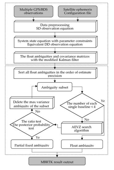
To address the aforementioned problems, a rigorous algorithm for MBRTK is presented in this paper to improve the RTK positioning accuracy and availability using multiple reference receivers, and a modified Kalman filter with parameter constraints is used to estimate the system states. Then, a PAR strategy for high-dimensional ambiguity is proposed to determine an ambiguity subset with high confidence. In order to validate and assess the performance of the proposed method, the positioning results of different satellite systems and reference stations are calculated and compared with the SBRTK.
This paper is organized as follows. In Section 2, conventional single-differenced (SD) and equivalent double-differenced (DD) observation equations are introduced. Then, a modified Kalman filter with parameter constraints is proposed. The redundancy of MBRTK is given, along with the data processing flow. In Section 3, the static and kinematic experiments are carried out and the impact of satellite systems as well as the reference receivers are discussed. Finally, our conclusions are summarized in Section 4.

2. Methodology

2.1. SD Observation Equations

As shown in Figure 1, there are four receivers tracking n satellites simultaneously, including three reference receivers r (r = a, b, and c) and one rover receiver u. It is preferable that the precise positions of three reference receivers are obtained in advance. Three reference receivers can be used to enhance the strength of the kinematic positioning model.
Without loss of simplicity, the SD observation equations of carrier phase and code observations for single satellite system can be presented as follows:
{ λ Δ φ a u s = Δ ρ a u s + c Δ t a u + λ Δ N a u s + Δ T a u s Δ I a u s + Δ ε a u s Δ P a u s = Δ ρ a u s + c Δ t a u + Δ T a u s + Δ I a u s + Δ ς a u s λ Δ φ b u s = Δ ρ b u s + c Δ t b u + λ Δ N b u s + Δ T b u s Δ I b u s + Δ ε b u s Δ P b u s = Δ ρ b u s + c Δ t b u + Δ T b u s + Δ I b u s + Δ ς b u s λ Δ φ c u s = Δ ρ c u s + c Δ t c u + λ Δ N c u s + Δ T c u s Δ I c u s + Δ ε c u s Δ P c u s = Δ ρ c u s + c Δ t c u + Δ T c u s + Δ I c u s + Δ ς c u s
where Δ ( ) r u = ( ) u ( ) r is the SD operator between reference receiver r and rover receiver u. The superscript s (s = j, k, …, n) denotes the satellite, and satellite j is set as the reference satellite. All satellites can be arranged with the descending order by satellite elevation angle. P and φ are the observations of code and carrier phase, respectively, and λ denotes the wavelength of the carrier. ρ is the geometric distance as a function of the receiver and satellite coordinates. c is the speed of light in vacuum. t represents user receiver clock error. N is the integer ambiguity of carrier phase. T and I are the tropospheric and ionospheric delay, whose difference can be ignored for short baseline. ς and ε are the measurement noise of code and carrier phase, respectively.
By combining SD observation equations of all satellites for single satellite system, the linearized equations in matrix formation can be represented as
v = A x + B N + C t L , P
where x is a column vector of coordinate corrections. N is a column vector of SD ambiguities. t is a column vector of SD receiver clock errors. A and C are the corresponding coefficient matrices, respectively. L is a column vector of the observation minus computation (OMC) terms. v is a vector of SD residual errors. P is a weight matrix of SD observations. The sub-matrices of the above matrices can be calculated by Equation (1) and the specific expressions can be derived as
A = [ A j A k A n ] ,   B = [ B j B k B n ] ,   C = [ C j C k C n ] ,   L = [ L j L k L n ] ,   v = [ v j v k v n ]
It is assumed that undifferenced observations are independent with elevation-dependent weights and their weight matrix is a diagonal matrix. The different SD observations among multiple receivers tracking the different satellite are not correlative. However, the different SD observations among multiple receivers tracking the identical satellites are correlative, which cannot be ignored. The SD weight matrix can be calculated exactly by the law of variance-covariance propagation. Thus, the weight matrix of Equation (2) is block-diagonal and can be derived as follows
P = d i a g ( P L j , P P j , P L k , P P k , , P L n , P P n )
where the sub-matrix P L s and P P s are the weight matrix of SD observations for carrier phase and code corresponding to single satellite s.
The specific expression of weight matrix for SD observations of single satellite s is as follows
P s = [ σ a s + σ u s σ u s σ u s σ u s σ b s + σ u s σ u s σ u s σ u s σ c s + σ u s ] 1
where σ s = a 0 + a 1 e θ s / 10 , σ s is the variance of undifferenced observation, and the symbol θ s is the satellite elevation angle with a 0 = 2 mm, a 1 = 4 mm for carrier phase and a 0 = 20 cm, a 1 = 40 cm for code, the cut-off elevation angle is set to 10°.

2.2. Equivalent DD Observation Equations

In Equation (2), the coordinate corrections and ambiguities are of interest, and the SD receiver clock errors can be eliminated directly from the observation equations based on equivalence principle [31,32]. Thus, the equivalent DD observation equations for single satellite system can be expressed as
{ R v = R A x + R B N R L , P R = E C ( C T P C ) 1 C T P
where E is an identity matrix. R is the transformation matrix of eliminating the clock errors with a rank defect of three. It means that the three SD ambiguities of reference satellite can be set to zero to keep the parameters independent, and the other SD ambiguities can be converted to the equivalent DD ambiguities.
Considering the GPS/BDS positioning, the equivalent DD observation equations of MBRTK can be obtained as
[ v G v C ] V = [ A G B G 0 A C 0 B C ] H [ x N G N C ] X [ L G L C ] Z , [ P G 0 0 P C ]
where the subscripts G and C denote the satellite system. A G = R G A G , A C = R C A C , B G = R G B G , B C = R C B C , L G = R G L G , L C = R C L C , v G = R G v G , v C = R C v C . x is a column vector of coordinate corrections, N G and N C are the column vector of the equivalent DD ambiguities for GPS and BDS systems.
As shown in Equation (7), the observations of four receivers can be modelled and processed strictly to obtain the positioning results of the MBRTK, which is not only equivalent to the conventional observation equations of the SBRTK, but also the correlative characteristics of differenced observations are solved clearly. If there are multiple reference and rover receivers tracking multiple satellites, the similar equations can be obtained for RTK positioning. As a special case, when there is only one reference receiver and one rover receiver, the equivalent DD equations can be reduced to the conventional DD equations of the SBRTK.

2.3. The Modified Kalman Filter

The Kalman filter is an optimal recursive estimator, which uses a dynamic model and sequential measurements to estimate the unknown state parameters in a minimum variance sense. In this paper, the constant velocity (CV) model [46] are adopted and the position–velocity components of the rover receiver and equivalent DD ambiguities are selected as system states. Let us still take Figure 1 as an example, the system states are expressed as follows:
X = [ x a u , v a u X a u , x b u , v b u X b u , x c u , v c u X c u , Δ N a u j k , Δ N a u j n N a u , Δ N b u j k , Δ N b u j n N b u , Δ N c u j k , Δ N c u j n N c u ] T
where X a u , X b u , and X c u are the position–velocity components of rover receiver, which are estimated corresponding to different reference receivers in Equation (7). In fact, the position–velocity components of rover receiver u for single epoch should be the same values, which can be as a constraint to enhance the strength of RTK positioning. N a u , N b u , and N c u are the corresponding equivalent DD ambiguities for three reference receivers, respectively.
Considering the redundant position–velocity components of rover receiver, a constraint equation can be expressed as:
[ 1 0 - 1 0 0 0 0 1 0 - 1 0 0 1 0 0 0 - 1 0 0 1 0 0 0 - 1 ] D 1 [ x a u v a u x b u v b u x c u v c u ] X 1 = [ 0 0 0 0 ] M 1
Equation (9) can be expanded as follows
[ D 1 0 0 0 ] D [ X 1 N ] X = [ M 1 0 ] M
Thus, based on Equations (7) and (10), the system state and observation equations of Kalman filter with parameter constraints are expressed as follows:
{ X t = Φ t , t 1 X t 1 + W t Z t = H t X t + V t D X t = M
where subscript t denotes the epoch, X t is the unknown state vector at epoch t, Φ t , t 1 is the state translation matrix from epoch t − 1 to t, W t is the noise vector of the system state model with zero mean and the covariance matrix Q w k , the setting of covariance matrix Q w k can refer to related literature such as Takasu. [47] and Zhao et al. [17] which is not discussed here. H t is the design matrix and Z t is column vector of the observation minus calculation (OMC) terms at epoch t, V t is a noise vector of observations with zero mean and the covariance matrix Q v k . Moreover, the noise W t and V t are assumed non-correlated.
The Kalman filter solution of the system states with constraint equation [48] is derived as
{ X ¯ t = Φ t , t 1 X t 1 Q ¯ t = Φ t , t 1 Q t 1 Φ t , t 1 T + Q w k X ¯ t = X ¯ t D T ( D D T ) 1 ( D X ¯ t M ) J t = Q ¯ t H t T ( H t Q ¯ t H t T + Q v k ) 1 X ^ t = X ¯ t + J t ( Z t H t X ¯ t ) Q X ^ t = Q ¯ t J t H t Q ¯ t
where X ¯ t and Q ¯ t are the predicted state vector and its corresponding predicted covariance matrix. X ¯ t is the corrected value of one-step predicted state vector, which can be improved using constraint equation. J t is the equivalent gain matrix, which can balance the observation and state information, X ^ t and Q X ^ t are the state estimation vector and its corresponding covariance matrix at epoch t. With more epoch-data accumulation, the Kalman filter solution will get better and better, and the float ambiguities are more precise in favor to improve the performance of AR.

2.4. The Redundancy of MBRTK

The redundancy is an important indicator to illustrate the reliability of the model, which is computed as the number of observations minus the number of unknown parameters for single epoch [49]. In Table 1, we give the number of observations, the number of unknown parameters and the redundancy of MBRTK compared with the SBRTK. Because the Doppler observations are not adopted to estimate the velocity parameters in Equation (7), the velocity components of system states are only predicted in the time update step and are not adjusted in the measurement update step of Kalman filter. Thus, the velocity state parameters are not considered for the calculation of redundancy in Table 1. g and b are the satellite number of single GPS and single BDS. r is the number of reference stations. Because of the equivalence between SBRTK and MBRTK, the condition of MBRTK is the same as the conventional SBRTK, as shown in the fifth column of Table 1. The redundancy is given based on the following assumptions, as (1) the ambiguities are estimated as time-continuous values, (2) the equivalent DD observation equations can be established in intra-system for both single GPS and single BDS, (3) multiple reference receivers can track the same satellites simultaneously.
As an example, considering the GPS/BDS model for MBRTK, the number of SD observations for both carrier phase and code is 2r(g + b). The number of unknown parameters consists of 3r receiver positions, r(g − 1) ambiguities for GPS, and r(b − 1) ambiguities for BDS. The number of observation redundancy is r(g + b − 1). If there are multiple reference receivers (r ≥ 2) with more data accumulated, the redundancy of MBRTK can increase rapidly, as well as 3(r − 1) constraint equations can be obtained, which can improve the estimable accuracy of unknown state parameters and enhance the strength of MBRTK. Generally, the more the number of reference receivers is, the greater the redundancy improvement is.

2.5. Data Processing Strategy

The data processing flow of MBRTK for single epoch is shown in Figure 2, which is divided into two main parts. The first part is data organization and parameter estimation. First, the observations of multiple reference and rover receivers are collected for MBRTK. Second, the SD observations between each reference and rover receivers are used to establish the SD observation equations. Then, the equivalent DD observation equations are obtained through the equivalent transform, and the modified system state equation with parameter constraints are performed to estimate the unknown state parameters. Finally, the float ambiguities and covariance matrices can be derived by the modified Kalman filter.
The second part of the data processing is AR of MBRTK. A modified PAR method is adopted to determine an ambiguity subset. First, the decorrelated ambiguities rather than raw float ambiguities are chosen, and the first subset is determined by reordering with the ascending estimate precision. Second, the number of valid ambiguities of every single-baseline is calculated. If the number of valid ambiguities is less than 4, only the float solution of MBRTK is available. Third, after the second step, all float ambiguities of MBRTK are used to fix a potential subset by the Agrell, Eriksson, Vardy, Zeger (AEVZ) search algorithm [42]. Fourth, the ratio test and the posterior probability test are calculated. If the subset passes the tests, the current ambiguity subset is accepted with sufficient confidence and the fixed solution of the MBRTK is available. On the contrary, if the last ambiguity with the lowest precision is rejected, the second step is repeated until the ambiguity solution of the MBRTK is determined. The critical criterion of ratio value and posterior probability are set to 2.0 and 0.90, respectively.

3. Validation and Analysis

In order to test the performance of the proposed MBRTK, we collect the static and kinematic dataset from Curtin University in Australia and Shandong University, Weihai in China, respectively. The static experiment is designed to validate the feasibility and reliability of the proposed MBRTK, and the kinematic experiment is to evaluate its positioning performance for different reference stations. The proposed MBRTK is compared with the conventional SBRTK with PAR method.

3.1. Static Experiment

3.1.1. Experiment Setup

A one-day dataset on 1 July 2018 of four stations (CUT00, CUTA0, CUTB0, and CUTC0) located at Curtin University in Australia, are collected for the data processing. The positions of four stations are precisely known, and each station is equipped with a TRM59800.00 SCIS antenna, which is connected with Trimble NetR9 receiver (Trimble Navigation Limited, Sunnyvale, CA, USA). Single-frequency code and carrier phase observation of the GPS L1 signal is adopted, and the sampling interval of the observation is 30 s. The satellite cut-off elevation angle is set to 10°. The distribution of four stations and the sky plot of station CUT00 is depicted in Figure 3. Three schemes are designed to calculate the precise position of CUT00, which are summarized in Table 2.

3.1.2. Analysis of Positioning Results

Figure 4 depicts the number of observed GPS satellites and redundancy, as well as the relative dilution of precision (RDOP) value of scheme-three during 1 July 2018. As shown, the average number of GPS observed satellites and redundancy is 7.6 and 16.9, respectively. The average RDOP value is 7.3 for the whole day.
Figure 5 shows the positioning errors in the North (N), East (E), and Up (U) components for three schemes, and the corresponding statistics are listed in Table 3. The results show that MBRTK has better positioning accuracy than SBRTK. The root mean square (RMS) values of the MBRTK for scheme-two and scheme-three are (2.4, 2.0 and 6.3) mm, and (2.2, 1.9 and 5.9) mm in N, E, and U components, while the corresponding values of the SBRTK are (2.8, 2.3 and 7.3) mm. The ambiguity-fixing rate of the three schemes are all 100%. Compared with the positioning results of the SBRTK, it is apparent that scheme-two and scheme-three have a performance improvement by approximately (14%, 13%, and 14%), and (21%, 17%, and 19%) in N, E, and U components, respectively, validating the feasibility and reliability of the proposed MBRTK.

3.2. Kinematic Experiment

3.2.1. Experiment Setup

The kinematic experiment is conducted at Shandong University, Weihai, on November 18, 2018 (from 12:53 to 14:10 UTC). The rover receiver (Trimble NetR9) and antenna (TRM57971.00) are installed on the top of a car, driving on the city roads of Weihai, which is marked as TBR9 as shown in Figure 6. Two reference receivers (Hi-Target VNet) and antenna (HX-AT2300) are located on the rooftop of the Wentian building in Shandong University, while the third reference receiver (South NetS9) and antenna (TRM57971.00) are located on the rooftop of a civil building in Weihai. The three receivers are marked as SDWA, SDWB, and SOTH, respectively. The linear distance of SDWA and SOTH is approximately 6.3 km, and a total number of approximately 4621 epochs of data are collected with 1 s sampling interval and 10° elevation cut-off angle. The trajectory of the car is shown in Figure 7.
In order to examine the performance of the proposed MBRTK, and compare the impacts of different satellite systems and reference receivers on the positioning results, six different schemes are conducted in this study. The differences between different schemes mainly focus on satellite systems and the number of reference receivers. The description of six positioning schemes is summarized in Table 4. Moreover, the reference coordinates of rover receiver can be calculated by Waypoint Inertial Explorer (IE) software 8.60 (NovAtel, Calgary, Alberta, Canada) for a forward-reverse model with three reference receivers [50], and the positioning errors are defined as the difference between positioning results and the reference coordinates. If the three-dimensional (3D) error of positioning is less than 10 cm, this epoch is defined to be successfully solved for the short baseline, and the availability of kinematic positioning is defined as the percentage of solved epochs of all epochs [38].

3.2.2. Positioning Results of Different Satellite Systems

To evaluate the performance of MBRTK for different satellite systems, the number of observed satellites and redundancy for the scheme-three, scheme-four and scheme-five are shown in Figure 8. In this contribution, G and C are denoted as system identifications for GPS and BDS, and R- is denoted as redundancy. The number of GPS and BDS satellites observed at one epoch over the whole observation segment is more than 6 and 9 mostly, and the total number of GPS/BDS satellites is more than 15. Meanwhile, the average redundancy is 7.6, 13.1, and 26.7 for the three different schemes, respectively. We can see that combined GPS/BDS system can significantly improve the redundancy of kinematic positioning, indicating combined GPS/BDS positioning has a strong ability to test the observations for modeling errors and improve the positioning accuracy.
Figure 9 shows the positioning errors of TBR9 after the first convergence for scheme-three, scheme-four, and scheme-five in N, E, and U components, respectively, and the success rate is marked on the graph. The statistics of three schemes are listed in Table 5. The RMS values of three different schemes are (5.5, 2.3, and 6.3) cm, (3.4, 1.6, and 5.7) cm, and (3.0, 1.5, and 4.6) cm in N, E, and U components, while the corresponding standard deviation (STD) values for three schemes are (3.7, 2.3, and 5.5) cm, (2.5, 1.5, and 4.7) cm, and (1.5, 1.4, and 3.9) cm. We can conclude that both the RMS and STD values of combined GPS/BDS system has a better positioning accuracy. Compared with RMS values of scheme-three and scheme-four, the RMS values of scheme-five have a performance improvement of approximately (45%, 35%, and 27%) and (12%, 6%, and 19%) in N, E, and U components, respectively. The STD values of scheme-five also have better consistency than those of scheme-three and scheme-four. Besides, the success rate of scheme-five is 94.4%, which has an availability improvement by approximately 33% and 10% compared with the success rate of scheme-three and scheme-four, respectively.

3.2.3. Positioning Results of Different Reference Receivers

To evaluate the performance of MBRTK for different number of reference receivers, the redundancy for the scheme-one, scheme-two, scheme-five and scheme-six are shown in Figure 10. The average redundancy for scheme-one and scheme-two is 9.4 and 9.3, which are almost the same because of the same processing strategy with the traditional SBRTK model, while the average redundancy for scheme-five and scheme-six with MBRTK is 26.7 and 40.0. The more the reference receivers are, the stronger the reliability of MBRTK model is. Meanwhile, the ADOP values [51,52] quantify the priori precision and geometry of ambiguities, which can be computed and illustrated in Figure 11 for the four schemes. We can see that, the ADOP values of all the four schemes can remain below 0.30 and 0.15 cycles for 99% and 90% of the observation segment, respectively. The ADOP values of scheme-five and scheme-six is the smaller than those of scheme-one and scheme-two, and scheme-six with three reference receivers has the optimal ADOP values. This is, thus, a promising indication that faster successful AR is possible for MBRTK model using multiple reference receivers.
Figure 12 shows the positioning errors of TBR9 after the first convergence for scheme-one, scheme-two, and scheme-six in N, E, and U components, respectively. Considering the positioning errors of scheme-five discussed in the previous section, the corresponding statistics of four schemes with different reference receivers are listed in Table 6. The RMS values of four different schemes are (3.3, 1.5, and 4.9) cm, (3.3, 1.8, and 5.4) cm, (3.0, 1.5, and 4.6) cm, and (3.0, 1.5, and 4.5) cm in N, E, and U components, respectively, while the corresponding STD values for four schemes are (1.9, 1.4, and 4.3) cm, (2.1, 1.5, and 4.2) cm, (1.5, 1.4, and 3.9) cm, and (1.5, 1.4, and 4.0).
From the analysis of the RMS and STD values, we can conclude that it is no statistically significant difference in the positioning errors for scheme-five and scheme-six, which can achieve a similar accuracy of 3.0 cm, 1.5 cm, and 4.5 cm level in N, E, and U components. Compared with the RMS values of scheme-one and scheme-two with SBRTK model, the RMS values of scheme-five and scheme-six with MBRTK model have a performance improvement by approximately (9%, 0%, and 6%) and (9%, 16%, and 16%) in N, E, and U components, respectively. Meanwhile, the STD values of scheme-five and scheme-six illustrate a better consistency than those of scheme-one and scheme-two. Besides, the success rate of four different schemes is 84.5%, 86.0%, 94.4% and 96.8%, respectively. Compared with scheme-one and scheme-two, the scheme-five and scheme-six have a similar availability improvement by approximately 10% in the success rate. However, it should be noted that scheme-six with three reference receivers does not present better performance than scheme-five with two reference receivers in both positioning accuracy and availability. The possible reason is that the reference receiver SDWB is close to the SDWA, which cannot further enhance the strength of the control network in the kinematic positioning.
Figure 13 presents L1/B1 carrier residuals for four schemes with different reference receivers. The DD residuals can be derived with the fixed coordinate parameters for MBRTK to compare with the residuals of SBRTK. It can be seen that the residuals of four schemes are randomly distributed along the zero Y-axis, and the mean values of the residuals are approximately 0 cm. The RMS and STD values of the residuals for scheme-one are worse than that of scheme-two. The possible reason is that there is a mountain behind the SDWA station, which leads to a worse satellite geometry than that of SOTH station. Although the residuals of scheme-six are slightly worse than that of scheme-five, the RMS and STD values of both schemes with multiple reference receivers have a good consistency, which are obviously smaller than that derived from scheme-one and scheme-two.

4. Discussion

The results of Section 3 indicate that the reference coordinates of rover receiver (TBR9) are calculated by Waypoint IE software 8.60 for a forward-reverse model with three reference receivers. However, the forward Kalman filter is applied to obtain the positioning results in MBRTK algorithm. The differences of model in the data processing would lead to a systematic positioning error, as shown in Table 6.
In addition, the positioning results of the forward-reverse model of IE software 8.60 still have the positioning error compared to the true position of rover receiver. Thus, to study the above differences, three additional schemes with different single reference receiver are conducted using the forward–reverse model by IE software 8.60. The statistics are listed in Table 7.
As can be seen, both the RMS and STD values of SDWA-TBR9 for IE software 8.60 can achieve the mm level and the positioning results are approximately equal to the reference coordinates of rover receiver by IE software 8.60. However, for the RMS and STD values of SDWB-TBR9 and SOTH-TBR9 using IE software 8.60, there is an obvious systematic error with cm level. That is to say, the reference coordinates by IE software 8.60 with three reference receivers are probably weighted average values based on the positioning results of SDWA-TBR9, SDWB-TBR9, and SOTH-TBR9, and the weight of SDWA-TBR9 is largest among the three single baselines. In other words, the reference coordinates of TBR9 are only relatively precise, but not absolutely accurate. It is worth noting that although the scheme-five and scheme-six still have a systematic error with cm level, the model of MBRTK is rigorous and reliable, which also have a higher success rate than those of three additional schemes by IE software 8.60.

5. Conclusions

In this paper, we present a new algorithm of MBRTK based on the equivalence principle for precise kinematic positioning. First, equivalent DD observation equations using SD observations are obtained through the equivalent transform to eliminate the receiver clock errors. Second, considering the redundancy of state information, a modified Kalman filter with parameter constraints is proposed to estimate the position–velocity states and equivalent DD ambiguities. The most outstanding feature of the MBRTK is that it has a rigorous model to solve the correlative characteristics of differenced observations for multiple reference receivers, as well as high positioning accuracy and availability could be achieved.
From the experiment and analysis, the following conclusions can be obtained:
(1)
For the static experiment, the MBRTK has better positioning accuracy than SBRTK. The MBRTK results with two and three reference receivers have the improvement of positioning accuracy by approximately (14%, 13%, and 14%), and (21%, 17%, and 19%) in N, E, and U components, respectively, validating the feasibility and reliability of the proposed MBRTK.
(2)
For the kinematic experiment, combined GPS/BDS positioning for MBRTK increases the number of available satellites and redundancy of the positioning model. Compared with single GPS and single BDS positioning, the combined GPS/BDS positioning has the accuracy improvement by approximately (45%, 35%, and 27%) and (12%, 6%, and 19%) in N, E, and U components and the availability improvement by approximately 33% and 10%, respectively.
(3)
For the analysis of reference receivers, the MBRTK model with multiple reference receivers can significantly increase the redundancy and provide the smaller ADOP values in favor to improve the performance of AR in comparison to the SBRTK model. The positioning results with two and three reference receivers can provide the similar accuracy of 3.0 cm, 1.5 cm, and 4.5 cm level in N, E, and U components, which have the accuracy improvement by approximately (9%, 0%, and 6%) and (9%, 16%, and 16%) compared with two SBRTK results, respectively. Meanwhile, the MBRTK results with two and three reference receivers have the availability improvement by approximately 10% in the success rate.
(4)
Due to the different models adopted by IE software 8.60 and MBRTK, there exists systematic errors between them. Compared with the positioning results of IE software 8.60 with one reference receiver, the MBRTK can achieve the stable accuracy with the cm-level, and have a rigorous and reliable model to keep a high availability of kinematic positioning.
Our future work will extend this algorithm to multi-frequency and multi-GNSS positioning considering the computational efficiency, and focus the distribution of multiple reference receivers to improve the precision, availability, and reliability of positioning results.

Author Contributions

J.W., T.X. and W.N. conceived and designed the experiments; J.W. performed the experiments, analyzed the data, and wrote the paper; T.X., W.N. and G.X. helped in the discussion and revision. All authors have read and agreed to the published version of the manuscript.

Funding

This study is financially supported by the National Natural Science Foundation of China (Grant No. 41874032, 41731069 and 41931076) and the National Key Research & Development Program of China (2016YFB0501701).

Acknowledgments

We are grateful to the anonymous reviewers and editors for their helpful and constructive suggestions, which significantly improved the paper quality. The authors would like to thank the Curtin GNSS Research Centre of Curtin University and the Center for Satellite Navigation and Remote Sensing of Shandong University, Weihai, for publicly sharing their GNSS data. Figure 7 is edited by using the Google Earth, which is also acknowledged.

Conflicts of Interest

The authors declare no conflict of interest.

References

  1. Yang, Y.; He, H.; Xu, G. Adaptively robust filtering for kinematic geodetic positioning. J. Geod. 2001, 75, 109–116. [Google Scholar] [CrossRef]
  2. Dong, D.; Bock, Y. Global positioning system network analysis with phase ambiguity resolution applied to crustal deformation studies in California. J. Geophys. Res. Solid Earth 1989, 94, 3949–3966. [Google Scholar] [CrossRef]
  3. Merrell, R. Application of GPS for transportation related engineering surveys. Bull. Geodesique. 1986, 60, 265–277. [Google Scholar] [CrossRef]
  4. Beckmann, A.; Larisch, H.; Schuster, O.; Barwinski, K. Engineering applications of GPS differential surveying. J. Surv. Eng. 1989, 115, 337–346. [Google Scholar] [CrossRef]
  5. Meng, X. From structural health monitoring to geo-hazard early warning: An integrated approach using GNSS positioning technology. In Earth Observation of Global Changes (EOGC); Lecture Notes in Geoinformation and Cartography; Krisp, J., Meng, L., Pail, R., Stilla, U., Eds.; Springer: Berlin/Heidelberg, Germany, 2013; pp. 285–293. [Google Scholar]
  6. Hofmann-Wellenhof, B.; Lichtenegger, H.; Wasle, E. GNSS—Global Navigation Satellite Systems—GPS, GLONASS, Galileo, and More; Springer: Berlin, Germany, 2008; pp. 397–414. [Google Scholar]
  7. Yang, Y.; Li, J.; Xu, J. Contribution of the Compass satellite navigation system to global PNT users. Chin. Sci. Bull. 2011, 56, 1733–1740. [Google Scholar] [CrossRef] [Green Version]
  8. Li, B. Review of triple-frequency GNSS: Ambiguity resolution, benefits and challenges. J. Glob. Position Syst. 2018, 16, 1. [Google Scholar] [CrossRef]
  9. Shi, C.; Zhao, Q.; Hu, Z.; Liu, J. Precise relative positioning using real tracking data from COMPASS GEO and IGSO satellites. GPS Solut. 2013, 17, 103–119. [Google Scholar] [CrossRef]
  10. Tu, R.; Liu, J.; Zhang, R.; Zhang, P.; Huang, X.; Lu, X. RTK model and positioning performance analysis using Galileo four-frequency observations. Adv. Space Res. 2018, 62, 913–926. [Google Scholar] [CrossRef]
  11. Teunissen, P.; Odolinski, R.; Odijk, D. Instantaneous BeiDou + GPS RTK positioning with high cut-off elevation angles. J. Geod. 2014, 88, 335–350. [Google Scholar] [CrossRef]
  12. Chen, H.; Xiao, Y.; Jiang, W.; Zhou, X.; Liu, H. An improved method for multi-GNSS baseline processing using single difference. Adv. Space Res. 2019, 63, 2711–2723. [Google Scholar] [CrossRef]
  13. Xi, R.; Meng, X.; Jiang, W.; An, X.; Chen, Q. GPS/GLONASS carrier phase elevation dependent stochastic modelling estimation and its application in bridge monitoring. Adv. Space Res. 2018, 62, 2566–2585. [Google Scholar] [CrossRef]
  14. He, H.; Li, J.; Yang, Y.; Xu, J.; Guo, H.; Wang, A. Performance assessment of single- and dual-frequency BeiDou/GPS single-epoch kinematic positioning. GPS Solut. 2014, 18, 393–403. [Google Scholar] [CrossRef]
  15. Deng, C.; Tang, W.; Liu, J.; Shi, C. Reliable single-epoch ambiguity resolution for short baselines using combined GPS/BeiDou system. GPS Solut. 2014, 18, 375–386. [Google Scholar] [CrossRef]
  16. Wang, M.; Cai, H.; Pan, Z. BDS/GPS relative positioning for long baseline with undifferenced observations. Adv. Space Res. 2014, 55, 113–124. [Google Scholar] [CrossRef]
  17. Zhao, S.; Cui, X.; Guan, F.; Lu, M. A Kalman filter-based short baseline RTK algorithm for single-frequency combination of GPS and BDS. Sensors 2014, 14, 15415–15433. [Google Scholar] [CrossRef]
  18. Liu, W.; Li, J.; Zeng, Q.; Guo, F.; Wu, R.; Zhang, X. An improved robust Kalman filtering strategy for GNSS kinematic positioning considering small cycle slips. Adv. Space Res. 2017, 63, 2724–2734. [Google Scholar] [CrossRef]
  19. Li, M.; He, K.; Xu, T.; Lu, B. Robust adaptive filter for shipborne kinematic positioning and velocity determination during the Baltic Sea experiment. GPS Solut. 2018, 22, 81. [Google Scholar] [CrossRef]
  20. Odolinski, R.; Teunissen, P.; Odijk, D. Combined BDS, Galileo, QZSS and GPS single-frequency RTK. GPS Solut. 2014, 19, 151–163. [Google Scholar] [CrossRef]
  21. Gao, W.; Gao, C.; Pan, S.; Meng, X.; Xia, Y. Inter-system differencing between GPS and BDS for medium-baseline RTK positioning. Remote Sens. 2017, 9, 948. [Google Scholar] [CrossRef] [Green Version]
  22. Wu, M.; Liu, W.; Wu, R.; Zhang, X. Tightly combined GPS/Galileo RTK for short and long baselines: Model and performance analysis. Adv. Space Res. 2018, 63, 2003–2020. [Google Scholar] [CrossRef]
  23. Hong, C.; Park, C.; Han, J.; Kwon, J. Medium to long range kinematic GPS positioning with position-velocity-acceleration model using multiple reference stations. Sensors 2015, 15, 16895–16909. [Google Scholar] [CrossRef]
  24. He, K.; Xu, G.; Xu, T.; Frank, F. GNSS navigation and positioning for the GEOHALO experiment in Italy. GPS Solut. 2016, 20, 215–224. [Google Scholar] [CrossRef]
  25. Paziewski, J. Precise GNSS single epoch positioning with multiple receiver configuration for medium-length baselines: Methodology and performance analysis. Meas. Sci. Technol. 2015, 26, 035002. [Google Scholar] [CrossRef]
  26. Bakuła, M. Constrained and network multi-receiver single epoch RTK positioning. Surv. Rev. 2018, 52, 1752–2706. [Google Scholar] [CrossRef]
  27. Fan, P.; Li, W.; Cui, X.; Lu, M. Precise and robust RTK-GNSS positioning in urban environments with dual-antenna configuration. Sensors 2019, 19, 3586. [Google Scholar] [CrossRef] [PubMed] [Green Version]
  28. Schaffrin, B.; Grafarend, E. Generating classes of equivalent linear models by nuisance parameter elimination, applications to GPS observations. Manuscr. Geod. 1986, 11, 262–271. [Google Scholar]
  29. Lindlohr, W.; Wells, D. GPS design using undifferenced carrier beat phase observations. Manuscr. Geod. 1985, 10, 255–295. [Google Scholar]
  30. Xu, G. GPS Data processing with equivalent observation equations. GPS Solut. 2002, 6, 28–33. [Google Scholar] [CrossRef]
  31. Xu, G. GPS: Theory, Algorithms and Applications; Springer: Berlin/Heidelberg, Germany, 2003; pp. 87–132. [Google Scholar]
  32. Shen, Y.; Xu, G. Simplified equivalent representation of GPS observation equations. GPS Solut. 2008, 12, 99–108. [Google Scholar] [CrossRef]
  33. Shen, Y.; Li, B.; Xu, G. Simplified equivalent multiple baseline solutions with elevation dependent weights. GPS Solut. 2009, 13, 165–171. [Google Scholar] [CrossRef]
  34. Wang, J.; Xu, T.; Nie, W.; Xu, G. A new algorithm for multi-baseline solution based on equivalence principle. Meas. Sci. Technol. 2020, accepted. [Google Scholar] [CrossRef]
  35. Parkins, A. Increasing GNSS RTK availability with a new single-epoch batch partial ambiguity resolution algorithm. GPS Solut. 2011, 15, 391–402. [Google Scholar] [CrossRef]
  36. Verhagen, S.; Li, B. LAMBDA Software Package: Matlab Implementation, Version 3.0; Delft University of Technology and Curtin University: Perth, Australia, 2012. [Google Scholar]
  37. Verhagen, S.; Li, B.; Teunissen, P. Ps-LAMBDA: Ambiguity success rate evaluation software for interferometric applications. Comput. Geosci. 2013, 54, 361–376. [Google Scholar] [CrossRef] [Green Version]
  38. Li, B.; Shen, Y.; Feng, Y.; Gao, W.; Yang, L. GNSS ambiguity resolution with controllable failure rate for long baseline network RTK. J. Geod. 2014, 88, 99–112. [Google Scholar] [CrossRef]
  39. Shi, J.; Gao, Y. A fast integer ambiguity resolution method for PPP. In Proceedings of the ION/GNSS 2012, Nashville, TN, USA, 17–21 September 2012. [Google Scholar]
  40. Li, P.; Zhang, X. Precise point positioning with partial ambiguity fixing. Sensors 2015, 15, 13627–13643. [Google Scholar] [CrossRef] [Green Version]
  41. Wang, J.; Feng, Y. Reliability of partial ambiguity fixing with multiple GNSS constellations. J. Geod. 2013, 87, 1–14. [Google Scholar] [CrossRef]
  42. Jazaeri, S.; Amiri-Simkooei, A.; Sharifi, M. Fast integer least-squares estimation for GNSS high-dimensional ambiguity resolution using lattice theory. J. Geod. 2012, 86, 123–136. [Google Scholar] [CrossRef] [Green Version]
  43. Teunissen, P. The least-squares ambiguity decorrelation adjustment: A method for fast GPS integer ambiguity estimation. J. Geod. 1995, 70, 65–82. [Google Scholar] [CrossRef]
  44. Chang, X.; Yang, X.; Zhou, T. MLAMBDA: A modified LAMBDA algorithm for integer least-squares estimation. J. Geod. 2005, 79, 552–565. [Google Scholar] [CrossRef] [Green Version]
  45. Wu, Z.; Bian, S. GNSS integer ambiguity validation based on posterior probability. J. Geod. 2015, 89, 961–977. [Google Scholar] [CrossRef]
  46. Schwarz, K.P.; Cannon, M.E.; Wong, R.V.C. A comparison of GPS kinematic models for the determination of position and velocity along a trajectory. Manuscr. Geod. 1989, 14, 345–353. [Google Scholar]
  47. Takasu, T.; Yasuda, A. Development of the low-cost RTK-GPS receiver with an open source program package RTKLIB. In Proceedings of the International Symposium on GPS/GNSS 2009, Jeju, Korea, 4–6 November 2009; pp. 1–6. [Google Scholar]
  48. Liu, Y.; Liu, J.; Zhu, D. Application of adaptive Kalman filter restricted by road information to vehicle-borne navigation. Geomat. Inf. Sci. Wuhan Univ. 2008, 33, 828–830. [Google Scholar]
  49. Odolinski, R.; Teunissen, P.; Odijk, D. Combined GPS + BDS for short to long baseline RTK positioning. Meas. Sci. Technol. 2015, 26, 045801. [Google Scholar] [CrossRef]
  50. Waypoint Products Group. A NovAtel Precise Positioning Product, Inertial Explorer User Guide, OM-20000106, Rev. 10. Available online: https://hexagondownloads.blob.core.windows.net/public/Novatel/assets/Documents/Waypoint/Downloads/InertialExplorer860_Manual/InertialExplorer860_Manual.pdf (accessed on 30 November 2014).
  51. Teunissen, P. A canonical theory for short GPS baselines. Part IV: Precision versus reliability. J. Geod. 1997, 71, 513–525. [Google Scholar] [CrossRef] [Green Version]
  52. Wang, K.; Chen, P.; Teunissen, P. Single-epoch, single-frequency multi-GNSS L5 RTK under high-elevation masking. Sensors 2019, 19, 1066. [Google Scholar] [CrossRef] [Green Version]
Figure 1. Four receivers track n satellites.
Remotesensing 12 03178 g001
Figure 2. A flowchart of data processing of the multi-baseline real-time kinematic (MBRTK) for single epoch where SD = single-differenced, DD = double-differenced, and AEVZ = Agrell, Eriksson, Vardy, Zeger.
Remotesensing 12 03178 g002
Figure 3. Distribution of four receivers (a) (http://saegnss2.curtin.edu.au/ldc/CU-GNSS-receivers-setup.pdf) and the sky plot (b) of the visible GPS satellites for station CUT00.
Remotesensing 12 03178 g003
Figure 4. Number of observed satellites and redundancy (left) and relative dilution of precision (RDOP) value (right) for static experiment.
Remotesensing 12 03178 g004
Figure 5. Errors in the East (E), North (N), and Up (U) of MBRTK for static experiment.
Remotesensing 12 03178 g005
Figure 6. The scene of rover receiver (a) and the reference receivers (b) on the rooftop of the Wentian building.
Remotesensing 12 03178 g006
Figure 7. The car trajectory of kinematic experiment for three reference receivers.
Remotesensing 12 03178 g007
Figure 8. Number of observed satellites (left) and redundancy (right) for three different schemes.
Remotesensing 12 03178 g008
Figure 9. Positioning errors for scheme-three, scheme-four, and scheme-five in N, E, and U components.
Remotesensing 12 03178 g009
Figure 10. Redundancy for four schemes with different reference receivers.
Remotesensing 12 03178 g010
Figure 11. Ambiguity dilution of precision (ADOP) values of four schemes with different reference receivers.
Remotesensing 12 03178 g011
Figure 12. Positioning errors for scheme-one, scheme-two, and scheme-six in N, E, and U components.
Remotesensing 12 03178 g012
Figure 13. L1/B1 carrier residuals for four schemes with different reference receivers.
Remotesensing 12 03178 g013
Table 1. The number of observations, unknowns, and redundancy for single epoch where SBRTK = single baseline real-time kinematic, MBRTK = multiple baseline real-time kinematic, GPS = global positioning system, and BDS = Beidou navigation system.
ModelNumber of ObservationsNumber of UnknownsNumber of RedundanciesNumber of ConstraintsCondition
SBRTK:GPS2(g − 1)3 + (g − 1)g − 40g ≥ 4
SBRTK:BDS2(b − 1)3 + (b − 1)b − 40b ≥ 4
SBRTK:GPS + BDS2(g − 1) + 2(b − 1)3 + (g − 1) + (b − 1)g + b − 50g ≥ 4 & b ≥ 4
MBRTK:GPS2rg3r + r(g − 1)r(g − 2)3(r − 1)g ≥ 4 & r ≥ 1
MBRTK:BDS2rb3r + r(b − 1)r(b − 2)3(r − 1)b ≥ 4 & r ≥ 1
MBRTK:GPS + BDS2r(g + b)3r + r(g − 1) + r(b − 1)r(g + b − 1)3(r − 1)g ≥ 4 & b ≥ 4 & r ≥ 1
Table 2. The description of the three schemes for static experiment.
SchemesReference StationsRover StationModel
OneCUTA0CUT00SBRTK
TwoCUTA0 + CUTB0CUT00MBRTK
ThreeCUTA0 + CUTB0 + CUTC0CUT00MBRTK
Table 3. Statistics of static experiment where RMS=root mean square.
SchemesRMS/mmImprovementNumber of EpochsSuccess Rate
NEUNEU
One2.82.37.3------2880100%
Two2.42.06.314%13%14%2880100%
Three2.21.95.921%17%19%2880100%
Table 4. The description of six positioning schemes.
SchemesReference StationsSystemsModel
OneSDWAGPS + BDSSBRTK
TwoSOTHGPS + BDSSBRTK
ThreeSDWA + SOTHGPSMBRTK
FourSDWA + SOTHBDSMBRTK
FiveSDWA + SOTHGPS + BDSMBRTK
SixSDWA + SDWB + SOTHGPS + BDSMBRTK
Table 5. Statistics of three schemes with different satellite systems for kinematic experiment where STD=standard deviation.
SchemesSystemsRMS/cmSTD/cmNumber of EpochsNumber of SuccessSuccess Rate
NEUNEU
ThreeGPS5.52.36.33.72.35.54621284061.5%
FourBDS3.41.65.72.51.54.74621390584.5%
FiveGPS/BDS3.01.54.61.51.43.94621436394.4%
Table 6. Statistics of four schemes with different reference stations for kinematic experiment.
SchemesModelRMS/cmSTD/cmNumber of EpochsNumber of SuccessSuccess Rate
NEUNEU
OneSBRTK3.31.54.91.91.44.34621390684.5%
TwoSBRTK3.31.85.42.11.54.24621397286.0%
FiveMBRTK3.01.54.61.51.43.94621436394.4%
SixMBRTK3.01.54.51.51.43.94621447196.8%
Table 7. Statistics of IE and MBRTK for kinematic experiment.
SchemesModelRMS/cmMean/cmNumber of EpochsNumber of SuccessSuccess Rate
NEUNEU
IE:SDWA-TBR9SBRTK0.50.80.80.0−0.10.14621402791.0%
IE:SDWB-TBR9SBRTK2.73.64.22.11.6−2.84621358877.6%
IE:SOTH-TBR9SBRTK1.63.03.11.62.2−2.34621410688.9%
MBRTK:FiveMBRTK3.01.54.6−2.7−0.6−2.54621436394.4%
MBRTK:SixMBRTK3.01.54.5−2.7−0.5−2.34621447196.8%

