Technical Note

Development of a Machine Learning-Based Radiometric Bias Correction for NOAA’s Microwave Integrated Retrieval System (MiRS)

Cooperative Institute for Satellite and Earth System Studies, Earth System Science Interdisciplinary Center, University of Maryland, College Park, MD 20742, USA
*
Author to whom correspondence should be addressed.
Remote Sens. 2020, 12(19), 3160; https://doi.org/10.3390/rs12193160
Submission received: 28 August 2020 / Revised: 22 September 2020 / Accepted: 24 September 2020 / Published: 26 September 2020

Abstract

:
We present the development of a dynamic over-ocean radiometric bias correction for the Microwave Integrated Retrieval System (MiRS) which accounts for spatial, temporal, spectral, and angular dependence of the systematic differences between observed and forward model-simulated radiances. The dynamic bias correction, which utilizes a deep neural network approach, is designed to incorporate dependence on the atmospheric and surface conditions that impact forward model biases. The approach utilizes collocations of observed Suomi National Polar-orbiting Partnership/Advanced Technology Microwave Sounder (SNPP/ATMS) radiances and European Centre for Medium-Range Weather Forecasts (ECMWF) model analyses which are used as input to the Community Radiative Transfer Model (CRTM) forward model to develop training data of radiometric biases. Analysis of the neural network performance indicates that in many channels, the dynamic bias is able to reproduce realistically both the spatial patterns of the original bias and its probability distribution function. Furthermore, retrieval impact experiments on independent data show that, compared with the baseline static bias correction, using the dynamic bias correction can improve temperature and water vapor profile retrievals, particularly in regions with higher Cloud Liquid Water (CLW) amounts. Ocean surface emissivity retrievals are also improved, for example at 23.8 GHz, showing an increase in correlation from 0.59 to 0.67 and a reduction of standard deviation from 0.035 to 0.026.

1. Introduction

1.1. MiRS

The Microwave Integrated Retrieval System (MiRS, https://www.star.nesdis.noaa.gov/mirs) has been the official operational microwave retrieval algorithm of the National Oceanic and Atmospheric Administration (NOAA) since 2007. Compared to visible and infrared radiation, microwaves have a longer wavelength, and thus can penetrate through the atmosphere more effectively. This feature allows microwave observations under almost all weather conditions, including in cloudy and rainy atmospheres. MiRS follows a one-dimensional variational (1DVAR) methodology [1,2]. The inversion is an iterative physical algorithm in which the fundamental physical attributes affecting the microwave observations are retrieved physically, including the profiles of atmospheric temperature, water vapor, non-precipitating cloud, hydrometeors, as well as surface emissivity and skin temperature [3]. The Joint Center for Satellite Data Assimilation (JCSDA) Community Radiative Transfer Model (CRTM) [4,5] is used as the forward and Jacobian operator to simulate the radiances at each iteration prior to fitting the measurements to within the combined instrument and forward model noise level. After the core parameters of the state vector are retrieved in the 1DVAR step, an additional post-processing is performed to retrieve derived parameters based on inputs from the core 1DVAR retrieval. The post processing products include total precipitable water (TPW), snow water equivalent (SWE), snowfall rate (SFR), surface precipitation rate, etc. [6]
MiRS has also been integrated into the Community Satellite Processing Package (CSPP), developed at the University of Wisconsin/Space Science and Engineering Center for users in the NOAA Direct Broadcast/Readout community. MiRS retrieval products are used routinely in operational weather analyses and forecasts, and also serve as inputs to downstream applications that are also used in operations. For example, MiRS water vapor profiles and TPW are used to generate the multi-satellite blended layer precipitable water and blended TPW products [7]. MiRS profiles of temperature and water vapor are also used as inputs to the tropical cyclone (TC) intensity estimation algorithm, the hurricane intensity and structure algorithm (HISA), developed at the Colorado State University/Cooperative Institute for Research in the Atmosphere (CSU/CIRA) [8] which is used operationally at the National Hurricane Center. Finally, MiRS precipitation rates are used as one of several satellite-based precipitation inputs to the NOAA Climate Prediction Center (CPC) Morphing Technique Algorithm (CMORPH) [9,10]. A schematic of the MiRS processing components and data flow is shown in Figure 1.

1.2. Radiometric Bias Correction

The mathematical basis for the inversion can be formulated as a minimization of a cost function. Two important assumptions are made for the minimization process, the local-linearity of the forward operator and the Gaussian nature of both the geophysical state vector and the simulated radiometric vector around the measured vector. However, the differences between the simulated radiometric vectors and the actual measurements can show significant biases, which can come from several sources. These include deficiencies in the forward model linking the atmospheric state to the radiative measurements (e.g., due to errors in the physics or spectroscopy), measurement errors (e.g., due to inadequacies in the characterization of instruments), and biases in the atmospheric state used as input to the forward model. Here, we assume that atmospheric state biases are small and focus on quantifying and removing biases due to forward model and measurement errors prior to use in the physical retrieval process.
Many efforts have been made to develop bias correction schemes for the numerical weather prediction (NWP) data assimilation (DA) systems and the physical retrieval systems which share the same bias removal scheme because both the DA and the retrieval systems are based on similar variational approaches and cost function minimization processes. For example, Auligné et al. and Zhu et al. [11,12] discussed the adaptive radiance observation bias correction scheme applied in the National Centers for Environmental Prediction’s (NCEP) Gridpoint Statistical Interpolation (GSI) data assimilation system, in which the variational air-mass bias component is estimated at the same time as the analysis control variables. A similar variational bias correction scheme for radiance data has been implemented and operational since 12 September 2006 at the European Centre for Medium-Range Weather Forecasts (ECMWF) [13,14].

1.3. Radiometric Bias Correction in MiRS

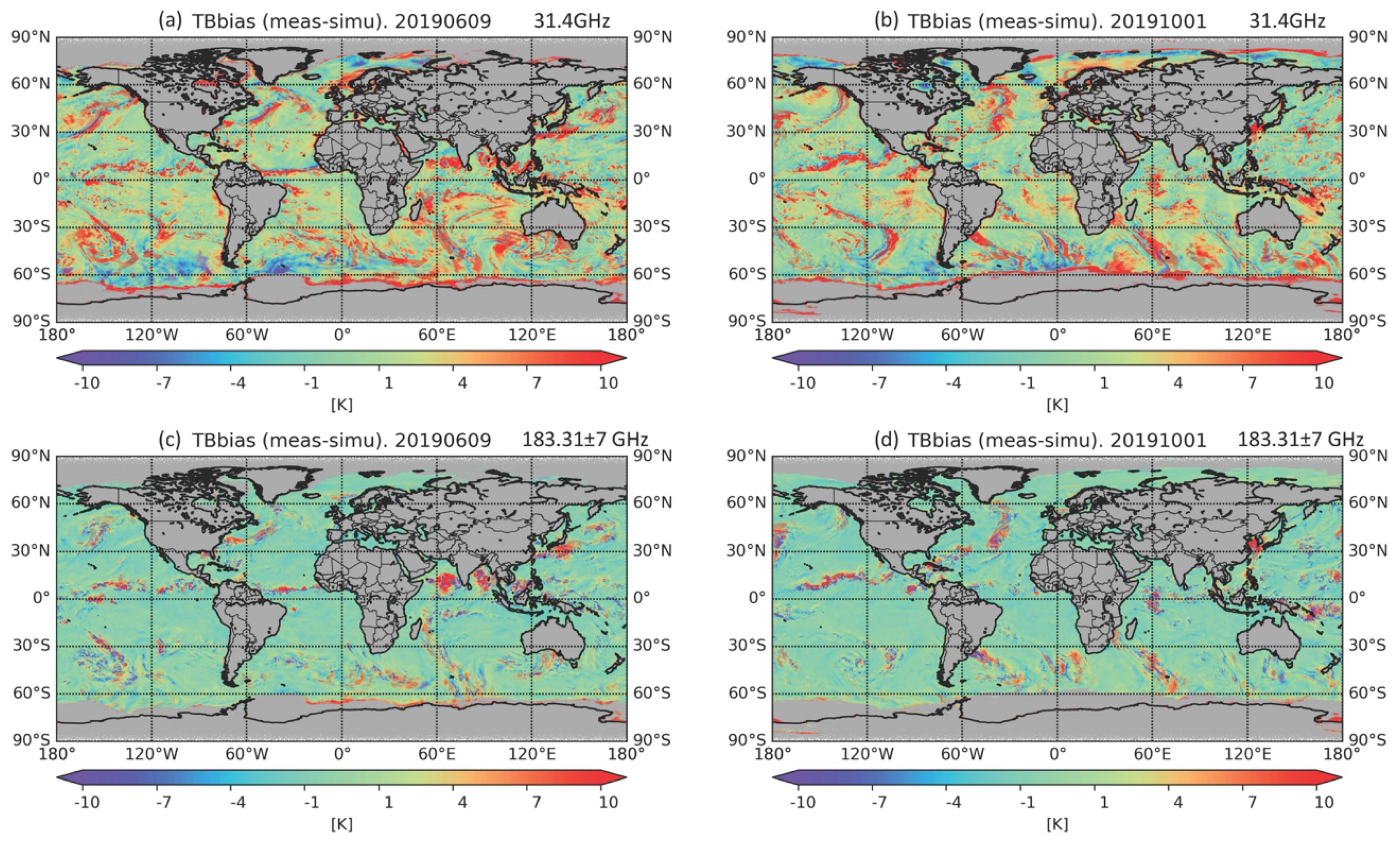
The current operational bias correction in MiRS is a procedure that applies a histogram adjustment to the radiative measurements to produce bias corrected radiances ready for inversion using a physical forward model (in this case, CRTM). This method, as inferred by its name, adjusts the histogram of the brightness temperature difference between simulated and observed radiances to make it centered around zero, which can reduce systematic errors in the retrievals related to forward and model and measurement biases. The histogram adjustment method specifies bias as a function of channel and scan position for each instrument, which means the bias does not change over time, and is static. However, in practice, the bias associated with a given instrument and frequency band generally varies in space and time, and may be air-mass or surface dependent at the time of the observation. For example, Figure 2 shows the global brightness temperature biases of Suomi National Polar-orbiting Partnership/Advanced Technology Microwave Sounder (SNPP/ATMS) over ocean, for two days ((9 June 2019 and 1 October 2019) at two different frequencies (31.4 GHz and 183.31 ± 7 GHz, i.e., ATMS channels 2 and 18, respectively), showing variability with spatial, temporal and spectral dependence. When the same scan-dependent biases are applied regardless of location or air-mass characteristics, the local variations of systematic errors would not be accounted for, which can then propagate into the retrieval variables. Therefore, replacement of the static bias correction scheme with a dynamic one that changes geographically and varies with atmospheric conditions can potentially reduce the errors of the retrieved parameters.

1.4. Neural Networks

Neural networks (NNs) have been widely used in the retrieval of geophysical parameters based on remote sensing data and other atmosphere science fields in recent years [15,16,17,18,19,20]. He et al. [21] studied two radiative bias correction methods developed through the correlation analysis between the microwave humidity and temperature sounder (MWHTS) measurements and air-mass. One method is linear regression, and the other is the neural network correction representing a nonlinear method. The authors found that the neural network correction outperformed the linear regression method in obtaining the desired bias; and by incorporating brightness temperatures corrected using a neural network approach in a one-dimensional variational system they could obtain higher retrieval accuracies of atmospheric temperature and humidity profiles. Considering the probable nonlinear nature of the difference between simulated and measured radiances, we choose neural networks as a new approach to implement a radiometric bias correction in MiRS system. The basic idea is to use NNs to learn the bias structure from historical collocations of simulated and measured brightness temperatures, along with the estimated corresponding atmospheric and surface state. The NN model, once trained, can then be used in near real time for bias correction during the retrieval process.
The remainder of this paper the contains the following outline: Section 2 contains a discussion of the datasets and methodology used in the study. The experimental design, including a description of the neural network and the MiRS algorithm, is contained in Section 3. Experimental results are highlighted in Section 4, which includes an evaluation of the neural network performance, an assessment of the impact of the neural network-derived bias corrections on MiRS retrieval performance, and some assessment of the neural network algorithm stability and robustness. Section 5 contains a summary and conclusions.

2. Materials and Methods

A Neural Network is a type of machine learning algorithm that is usually used in supervised learning. In supervised learning, a training dataset is given in which each set of input variables (or predictors) is corresponding to an already known output. The purpose of the neural network is to find the relationship between the predictors and the outputs in the training dataset. When a new dataset is provided (testing dataset), predictions are made by applying the learned relationship on predictors from the testing dataset. A deep neural network (DNN) is used in this research to simulate and predict the brightness temperature difference (between simulated radiance and actual measurements, labeled here as TBbias) for the advanced technology microwave sounder (ATMS) onboard the Suomi National Polar-orbiting Partnership (SNPP) satellite. A description of the SNPP/ATMS will be provided in Section 2.1, followed by discussion of how the training and testing datasets were assembled in Section 2.2, and a description of the validation dataset in Section 2.3.

2.1. Satellite and Sensor

The SNPP/ATMS data quality has been carefully evaluated [22,23], and its impact on the European Centre for Medium-Range Weather Forecasts (ECMWF) system and the United Kingdom’s Met Office numerical weather forecast was reported by Bormann et al. [24] and Doherty et al. [25], respectively. SNPP is the first of a series of the next-generation U.S. polar-orbiting satellites, which was launched in October 2011 and continues to be operated by NOAA until present. SNPP is the result of a partnership between NOAA and the National Aeronautics and Space Administration (NASA). It is designed to collect data on long-term climate change and short-term weather conditions to extend and improve upon data records established by the NASA’s Earth Observing System. SNPP was designed as a preparatory mission for the Joint Polar Satellite System (JPSS) series of satellites, all of which will also fly an ATMS instrument. The first satellite of the JPSS series (NOAA-20) was launched in November 2017 and is currently operational along with SNPP.
ATMS is a cross-track scanning instrument, with 22 channels at frequencies ranging from 23 to 183 GHz, which allows for profiling the atmospheric temperature/moisture, as well as providing information on clouds, non-precipitating clouds, and surface characteristics under clear-sky and cloudy conditions. In precipitating conditions, several channels can also provide information on liquid and frozen hydrometeors, which is indirectly related to the surface precipitation rate. In clear and cloudy (non-precipitating) conditions, channels at 23, 31 50, 88, and 165 GHz can provide information on total column water vapor, surface conditions and cloudiness. Channels between 50 and 60 GHz are used for atmospheric temperature sounding from the surface to about 1 hPa, while channels around 183 GHz provide information on the water vapor profile from the surface to about 200 hPa. Channels at 88 and 165 GHz provide significant information on the presence of rain and ice hydrometeors. Table 1 provides channel characteristics of all 22 ATMS channels, including central frequency, polarization, beam width, noise equivalent differential temperature (NEΔT), and the peak weight function (WF).

2.2. NN Training and Testing Datasets

Brightness temperature bias along with the concurrent SNPP/ATMS measured brightness temperature for 22 channels, satellite viewing angle, latitude, and other geophysical parameters including cloud liquid water (CLW), total precipitable water (TPW), and skin temperature (Tskin) have been used to establish the NN training and testing datasets. All of these parameters are collected over ocean. A data screening was applied in the training dataset which required that only brightness temperature biases less than 30K were included in the training set. The reason for the 30K limit is that such a large difference between observation and simulation indicates likely scattering or precipitation. In these cases, we do not have confidence that the NWP representation of the rain or ice particles is accurate enough to provide a reliable input to the CRTM simulation. (As noted in Section 3.2, the MiRS retrieval approach allows for the determination of highly scattering (precipitating) conditions and in these cases a bias correction is not applied due to large uncertainties in the forward modeling.) The training dataset contains 12 days with one-day from each month of either 2018 or 2019 (Table 2). The CLW, TPW, and Tskin for training were from the ECMWF analyses. Once the NN bias correction model was trained, the impact assessment was done on an independent day, 1 October 2019 for all ocean scenes between 55 S to 55N latitude. The purpose of the latitude limit is to avoid sea ice covered areas where surface emissivity is not well simulated. Since in operational application MiRS does not use any real-time data from NWP model forecasts or analyses, such as those from ECMWF, in the impact assessment testing experiments these three parameters were calculated either by a regression scheme (CLW) or by neural networks constructed for TPW and Tskin, respectively. The inputs for calculating them were brightness temperature measurements and geolocation parameters like satellite viewing angle and latitude. The training and testing data were selected based on the availability of the SNPP/ATMS measurements and our computational resources. Further details of the NN training and testing are contained in Section 3 and Section 4.

2.3. MiRS Retrieval Validation Dataset

To evaluate the impact of the new radiometric bias correction scheme, most of the MiRS retrievals, including atmospheric temperature profiles, water vapor profiles, CLW, TPW, and Tskin were validated with the ECMWF analyses. The ECMWF analyses are originally specified on 90 vertical pressure layers and at a 0.25-degree horizontal resolution. MiRS interpolates the analyses vertically into the 100 CRTM layers (from the surface to 0.01 hPa), and horizontally averages to 1 degree for the collocation with the ATMS measurement locations. Validation for the MiRS surface emissivity over the ocean at all channels was performed against the fast microwave emissivity model (FASTEM) [26] that takes the ECMWF analyses of wind speed, frequency, and observation zenith angle as inputs. In MiRS, ECMWF and other operational NWP data sets are used only for calibration in the radiance processing and in the retrieved product monitoring. They are not used in the 1DVAR inversion process. As the bias correction was developed for over-ocean measurements only, this paper evaluates MiRS retrievals performance of SNPP/ATMS over ocean only. Over other surfaces, the operational static bias correction scheme remained unchanged, therefore producing no impact on the MiRS retrievals over land, snow, and sea-ice scenes.

3. Algorithm and Experiment Design

3.1. MiRS Algorithm

The MiRS is an iterative, physically-based retrieval system based on 1DVAR inversion. The 1DVAR physical principle is to minimize a cost function (Equation (1)). The first item on the right side of Equation 1 represents the departure of state vector X to be retrieved from background X0, weighted by background error covariance matrix B. The second item represents the departure of simulated radiance Y from the observed radiance Ym, weighted by instrument and radiative transfer modelling error E. CRTM is the forward and adjoint operator used to generate simulated radiance Y, as well as the Jacobians (derivatives) which is the radiance response to a unit perturbation of the state vector. Minimization of the cost function is an iterative process with convergence reached if chi-squared metric, χ2, is less than or equal to 1 (Equation (2)). The iterative loop is also ended if the chi-squared metric does not meet the convergence criterion within 7 iterations. In practice, the global convergence rates approach 95% [27].
J ( X ) = [ 1 2 ( X X 0 ) T × B 1 × ( X X 0 ) ] + [ 1 2 ( Y m Y ( X ) ) T × E 1 × ( Y m Y ( X ) ) ]
χ 2 = ( Y m Y ( X ) ) T × E 1 × ( Y m Y ( X ) )

3.2. Experiment Design

This research chose a 4-layer neural network (with two hidden layers) to predict brightness temperature biases (22 channels). There are 200 neurons in each hidden layer, with a Rectified Linear Unit (ReLU) as the activation function, which is the most successful and widely-used activation function thus far in the deep learning community [28]. This configuration of layers, nodes and activation function was selected after extensive testing with smaller and larger numbers of layers and nodes, and with different activation functions such as Sigmoid and Leaky ReLU. The NN design used here produced the best results in terms of reproducing the observed biases. The optimizer used in this NN is RMSprop, with the learning rate of 0.001. Another problem with training neural networks is to choose the number of training epochs. Too many epochs can lead to overfitting, while too few could result in an underfit model. In the present study, early stopping was the method used to terminate training before overfitting occurred. This method split the training dataset and used a subset (in this study, 20%) as a validation dataset to monitor performance of the neural network model during training. An arbitrary large number of training epochs (or maximum number of epochs) was specified, and the training would be stopped if the loss on the validation dataset did not change over a given number of epochs (or patience). The maximum number of epochs and the patience used in this study were 1000 and 100, respectively.
The input layer has 27 variables over ocean, which includes SNPP/ATMS measured brightness temperature (22 channels), satellite viewing angle, latitude, CLW, TPW, and Tskin. Normalization of the input variables to a standard scale would allow the neural network to more quickly learn the optimal weights and biases. All of the 27 input variables were normalized by their respective mean and standard deviation calculated from the training dataset. Data screening was also applied which required that only observations where brightness temperature biases less than 30K were included in the training dataset. The output layer has 22 variables, representing brightness temperature biases for each of the 22 channels. The neural network was applied for all ocean scenes on the testing day. MiRS has the flexibility to choose the bias correction method for each channel. NN predicted brightness temperature biases were applied to SNPP/ATMS channels 1–15 plus 17 over ocean. All other channels used the static bias correction method. This choice of which channels the NN correction was applied to was based on a large number of sensitivity tests where the impact on retrievals was quantified. Finally, the MiRS retrieval approach structures the retrieval and state vector based on whether hydrometeor scattering is determined to be significant. In this study, bias corrections are only applied in conditions of little to no scattering (i.e., clear and cloudy/light rain scenes), as development of bias corrections for scenes with significant scattering and/or precipitation is a more challenging task.

4. Results

4.1. Neural Network Performance

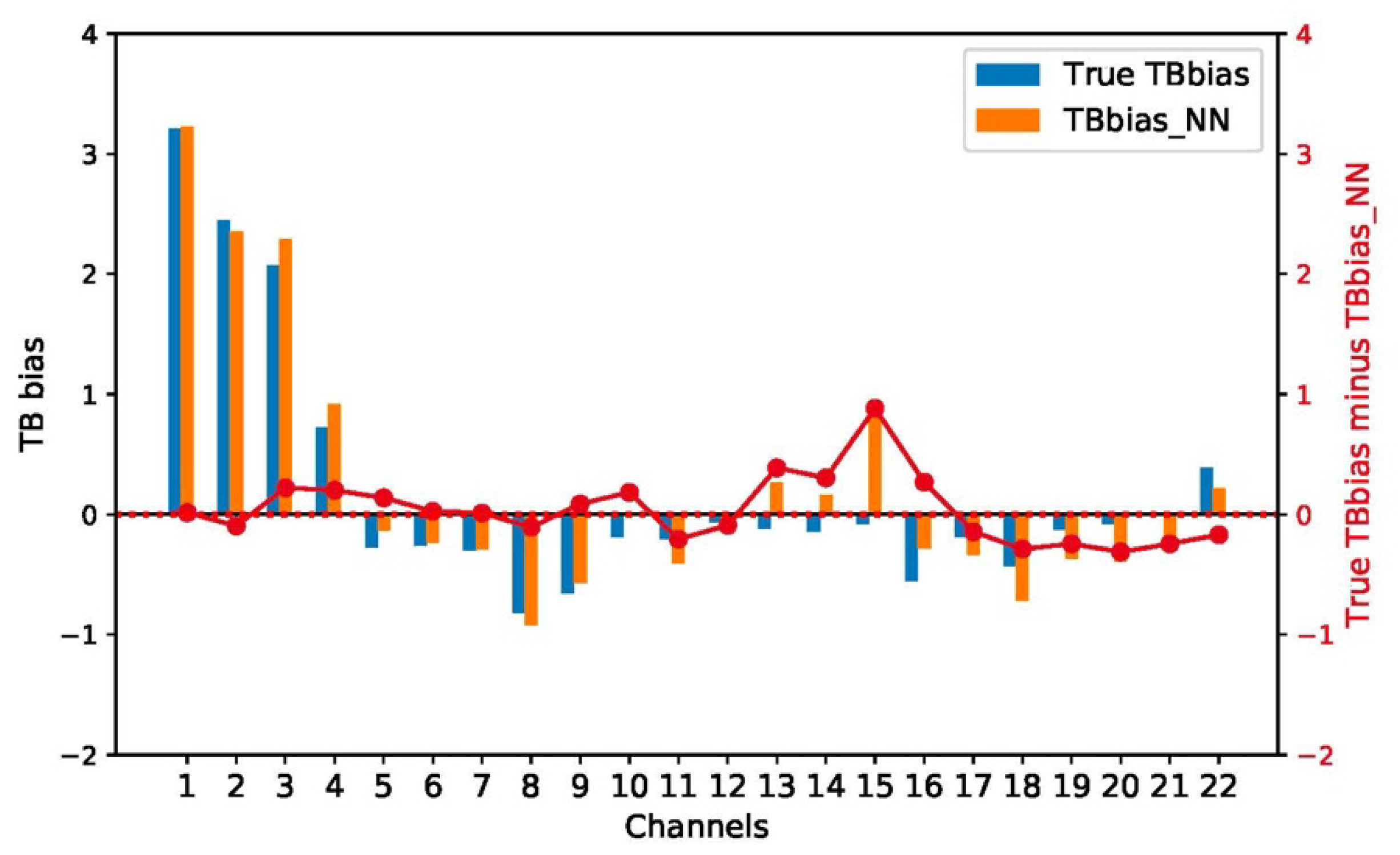
The neural network prediction of the brightness temperature bias of SNPP/ATMS was first validated with the true bias (measurements minus simulations) for one single day, 1 October 2019, as shown in Figure 3. The bars represent the mean true bias (blue) and NN predicted bias (orange) for each of the 22 SNPP/ATMS channels, with left y-axis showing their values. The difference between the mean NN predicted and true biases is presented by the red line with right y-axis showing its value. Only profiles with biases less than 30 K and located between 55 S and 55 N latitude over ocean are used in the averaging. Except for Channel 15, the differences between the NN prediction and true bias are less than 0.38. Channel 15 differences may be larger due to the peak height of its weighting function, which is approximately 2 hPa (~ 45 km altitude) where both the ECMWF model analyses and CRTM simulations may be less reliable.
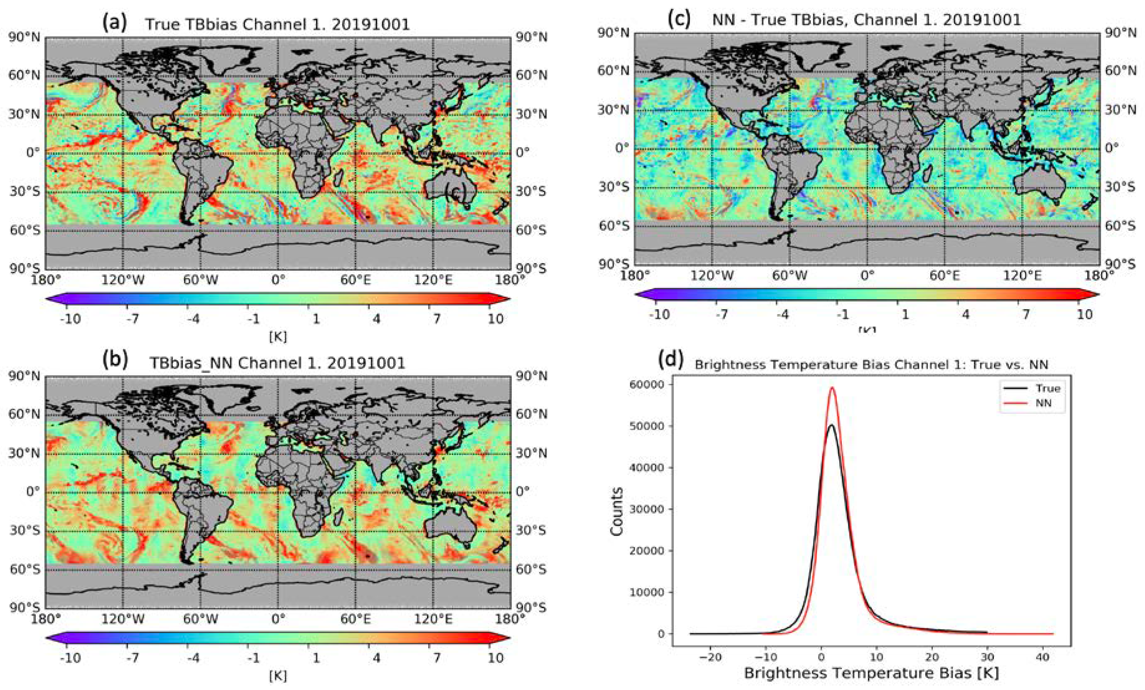
The performance for Channels 1–12 is generally good, with Channels 1, 6, and 7 having the smallest difference. For example, the averaged difference between NN predicted and true bias is about 0.01 K for Channel 1 (23.8 GHz), and their spatial patterns are very similar (Figure 4a,b). Figure 4 shows the brightness temperature bias maps of Channel 1 (23.8 GHz) for true values (a), NN prediction (b), and the difference between NN and true values (c), over ocean for latitudes between 55 S and 55 N. Quantitatively, the NN prediction matches the true bias special pattern very well. However, the NN estimates miss some cold features (blue color) in the midlatitudes and show warmer patterns over the south Pacific Ocean. It also shows slight scan angle dependency over the tropics despite using scan angle as one of the NN inputs aimed at minimizing this dependency. The histogram of the NN prediction is compared with that of the true bias (red vs. black in Figure 4d). The NN prediction does not capture the extreme cold bias less than −10 K and has fewer points between 0 K to −10 K, while it has more profiles around the peak (about 2 K) and contains a small number of points with a predicted warm bias higher than 30 K.

4.2. MiRS Retrievals

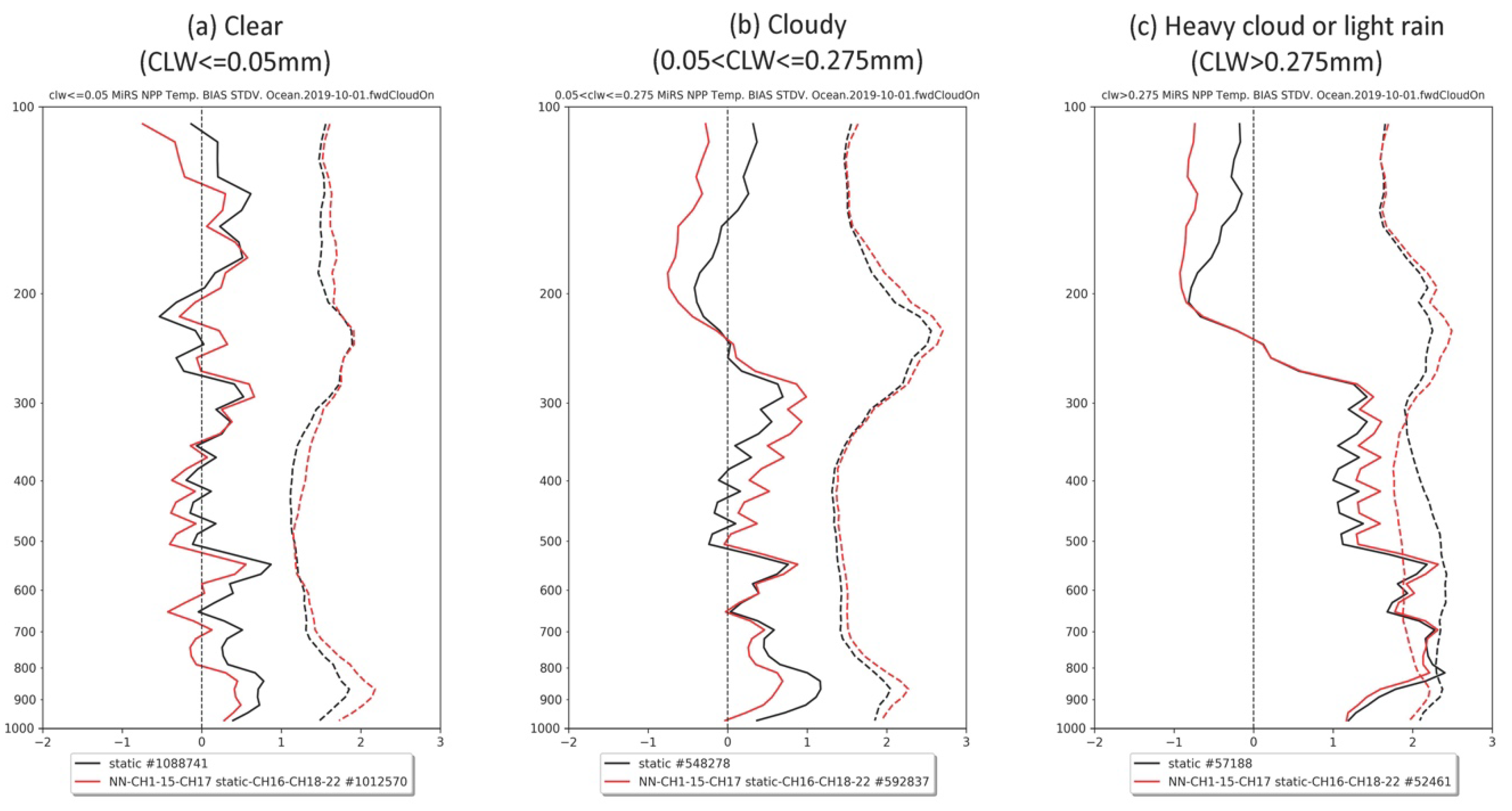
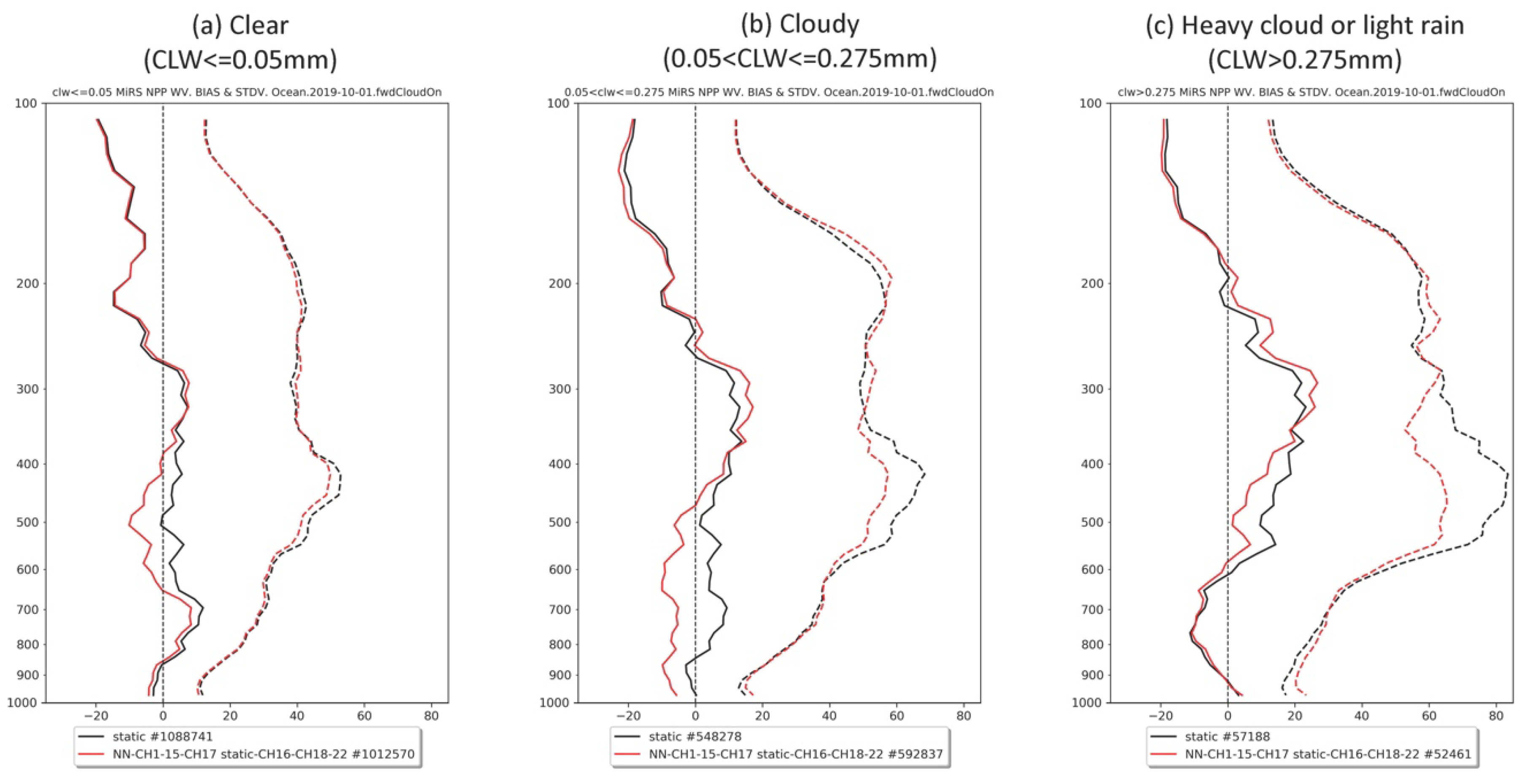
With MiRS using static bias correction as the baseline experiment (named as Static), an assessment of the impact of the neural network-derived bias corrections on MiRS retrieval performance over ocean is presented (named as NN). The MiRS retrieval performance of atmospheric temperature profiles for Static (black) and NN (red) are shown in Figure 5, with solid lines for bias and dashed lines for standard deviation, verified with ECMWF analyses between 1000–100 hPa. This verification was stratified by CLW amount into three scenarios: clear (CLW ≤ 0.05 mm), cloudy (0.05 ≤ CLW ≤ 0.275 mm), and heavy cloud or light rain (CLW > 0.275 mm), corresponding to Figure 5a–c. The sample sizes for each experiment under each scenario are given in the legend. In the clear and cloudy scenarios, impact of NN bias correction was similar, both with slightly reduced bias below 700 hPa and with slightly increased standard deviation at almost all levels. In the heavy cloud or light rain scenario, NN shows significantly reduced standard deviation under 300 hPa, with about 0.5 K smaller standard deviation at 650 hPa. Since the baseline static bias correction is developed using clear sky measurements only, it is perhaps expected that the largest and most positive impact of the NN bias correction is for scenes with significant cloudiness and/or light precipitation.
Similar profile plots for water vapor are shown in Figure 6, while the x-axis represents the percentage changes of bias and standard deviation with respect to ECMWF analysis at each layer. In the clear scenario, the NN bias percentage increased in magnitude about 5–10% between 700 hPa and 400 hPa compared with static experiment, while the standard deviation percentage decreased about 3% near 500 hPa. In the cloudy scenario, the bias percentage magnitude of the NN experiment is larger than Static at almost all levels, while the standard deviation is about 5–10% less than static between 600 hPa and 400 hPa. And in the heavy cloud or light rain scenario, NN water vapor bias slight decreased between 600 hPa and 350 hPa but increased between 350 hPa and 200 hPa. The most dramatic change is the NN standard deviation, which reduced from 80% to 60% between 600 hPa and 300 hPa. In summary, the MiRS water vapor retrieval using NN bias correction showed significantly reduced standard deviation at the middle levels. Similar, to the temperature profile results the largest positive impacts appear to be for cases with significant cloudiness and/or light rain.
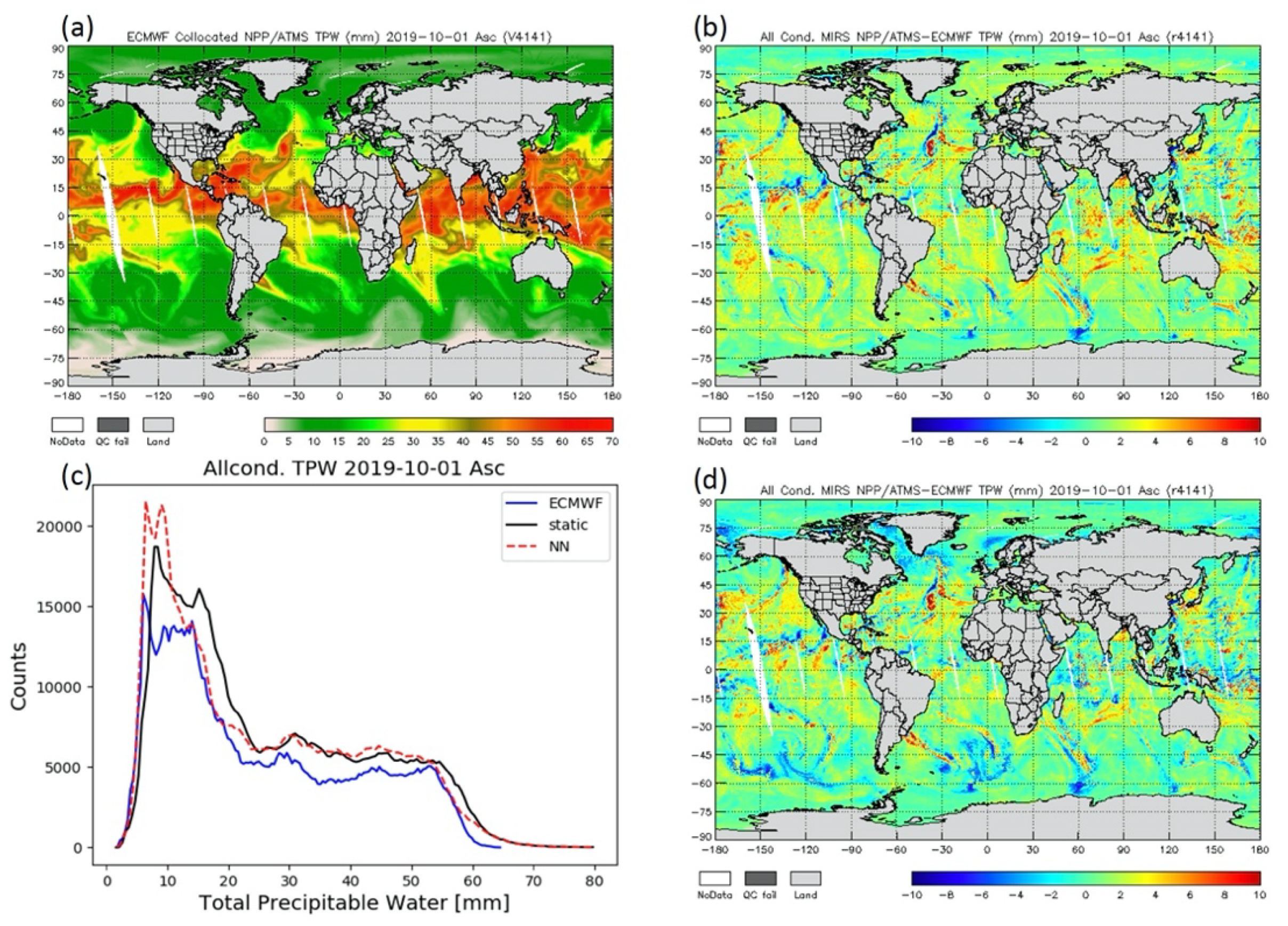
MiRS retrieval performance for two-dimensional variables TPW, Tskin, and surface emissivity is presented in the following figures and tables. The TPW map of ECMWF analysis collocated with the SNPP/ATMS ascending node over ocean is shown in Figure 7a. The MiRS TPW bias with ECMWF analysis from static and NN is shown in Figure 7b,d, and the histograms of ECMWF (blue), static (black), and NN (dashed red) are given in Figure 7c. Relative to ECMWF, static has a moist bias, while a drier bias is observed on the NN bias map, especially over high mid-latitude ocean in the Southern Hemisphere. In the histogram plot, the NN TPW is drier and closer to ECMWF analysis, especially between 0-5, 15–25, and 55–60 mm. The validation statistics of static and NN TPW are shown in the top left panel of Table 3. TPW from NN experiment shows dramatically smaller bias and a slight increase in standard deviation.
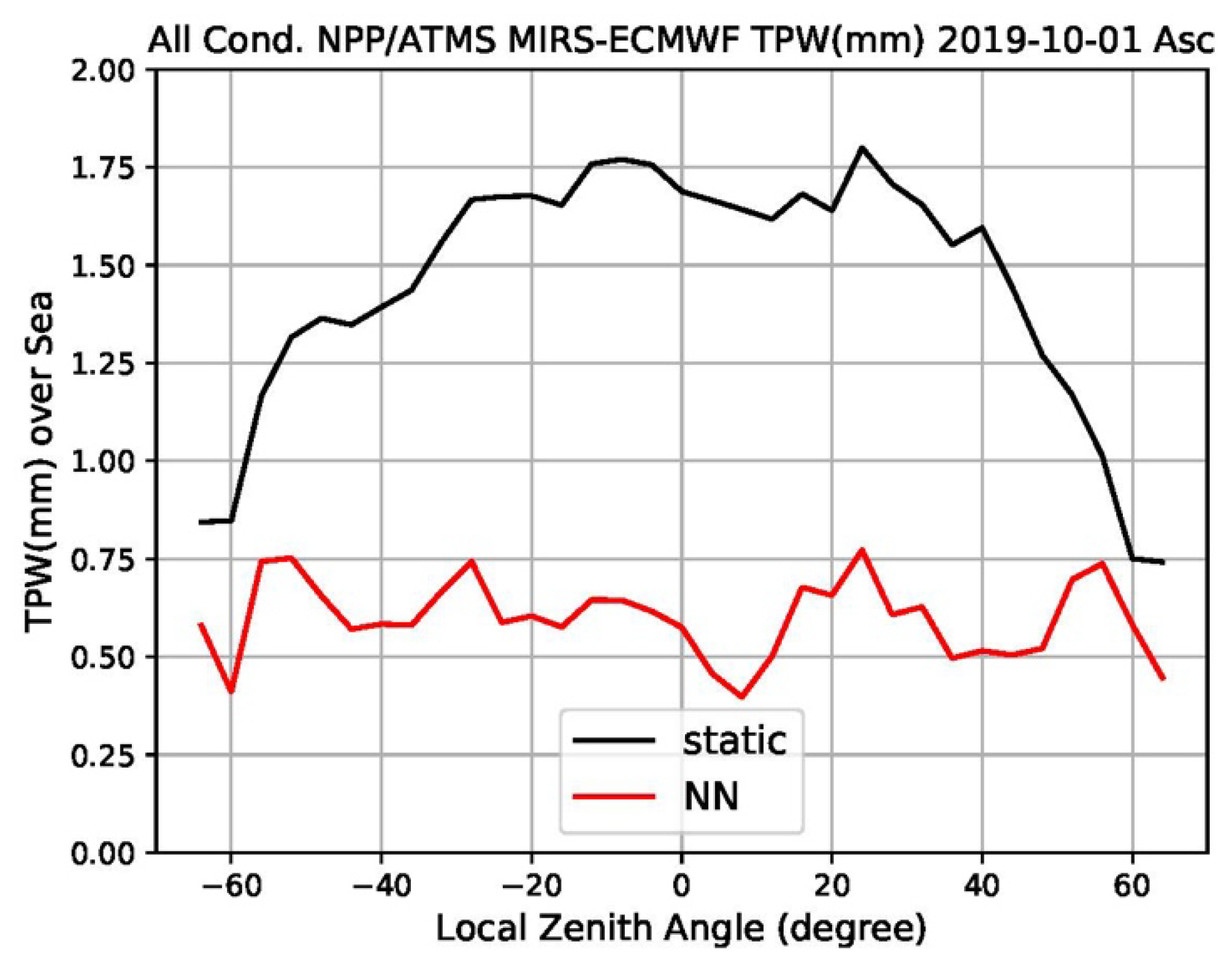
The MiRS SNPP/ATMS TPW local zenith angle dependency over ocean is presented in Figure 8, with the local zenith angle within −70 to 70 degrees along the x-axis and the bias between static (black) or NN (red) and ECMWF on the y-axis. NN has smaller biases than static at all angles, and it almost has no scan angle dependency. In contrast, TPW bias from static is larger at and near nadir and quickly drops from 1.75 mm to 0.75 mm when it reaches the edges of the scan. This significant improvement is likely due to the explicit accounting of scan angle and other geophysical variables in the NN bias correction model.
Table 3 shows the performance metrics of MiRS TPW, Tskin, and emissivity at 23.8 GHz and 88.2 GHz for SNPP/ATMS on 1 October 2019 over ocean, ascending node. The metrics include correlation, bias, and standard deviation validated against the ECMWF analysis (and FASTEM5 for emissivity), as well as the percentage change of these metrics from NN to Static. The numbers inside parentheses are sample sizes for each parameter and each experiment. Except for emissivity at 23.8 GHz, other parameters from NN have 0% or 1% increase in correlation comparing with Static, and a 60–80% decrease in bias. The standard deviation of TPW from NN is 12.9% greater, while there is a very small impact on Tskin and emissivity at 88.2 GHz.
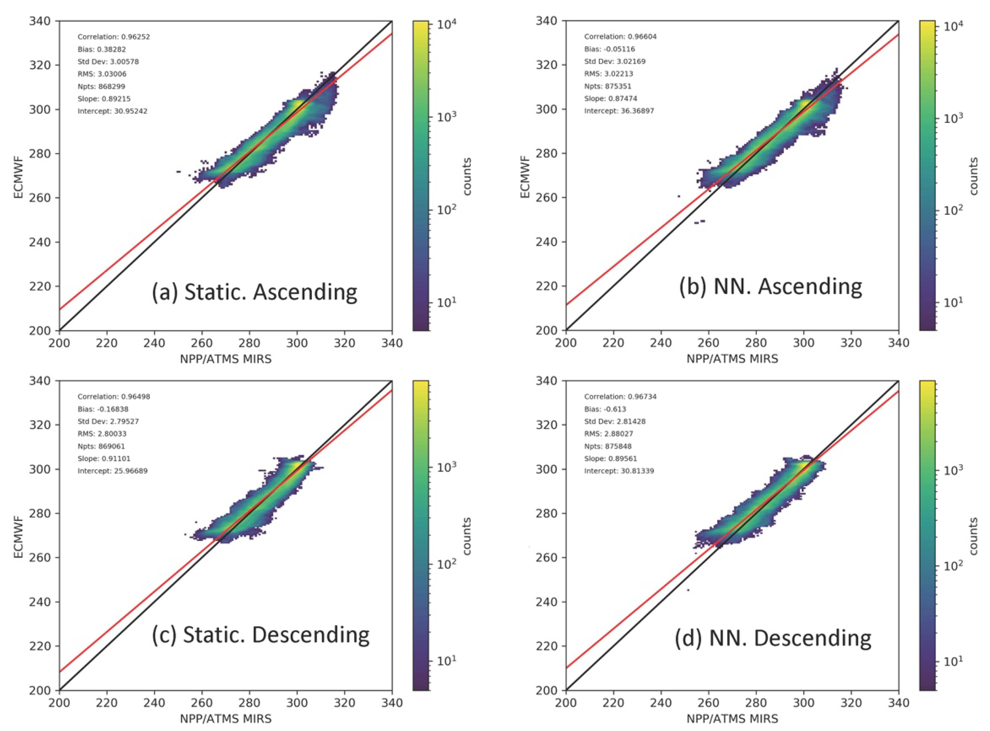
Results for performance metrics of descending node are similar to Table 3 except for Tskin, which has strong diurnal cycle. In Figure 9, MiRS Tskin retrievals are verified with ECMWF analyses and shown by density scatterplots. Tskin for static (left) and NN (right) are shown for both ascending (top) and descending (bottom) nodes. In ascending node, the bias from NN decreases from ~0.4 K to ~0.1 K. However, in descending node, the bias increases from ~−0.2 K to −0.6 K.
Overall, the impact of applying the NN bias correction has a positive impact on the retrievals of several key retrieval parameters, depending on the performance statistic, but atmospheric and surface conditions appear to modulate significantly the magnitude and sign (improvement or degradation) of the impacts.

5. Conclusions

We report on preliminary results of applying a machine learning approach to estimation of the radiometric bias correction of passive microwave measurements from the SNPP/ATMS instrument. The bias correction was based on collocations of ATMS data with ECMWF operational analyses in conjunction with the FASTEM5 ocean surface emissivity model. A neural network model was used to estimate the bias corrections, and the model explicitly includes impacts from surface and atmospheric conditions, as well as scan angle and frequency dependence. Furthermore, the NN bias corrections were tested in the MiRS retrieval system to assess the impact of the bias corrections relative to retrievals using the operational static bias corrections. Because of this NN formulation the bias correction model is dynamic, adjusting the bias prediction with each scene or field of view, in contrast to the static bias correction.
The impact study examined retrieval performance of vertical temperature and water vapor profiles, total precipitable water, skin temperature, and surface emissivity. For temperature, largest positive impacts of using the NN bias correction appeared focused in scenes with higher amounts of cloud (>0.275 mm) and/or light precipitation. Lower tropospheric temperature bias was also reduced for scenes with fewer clouds. For water vapor, the largest positive impacts were on the error standard deviation concentrated in the 600–300 hPa layer. The impact on the water vapor bias was mixed, with some layers showing improvement, and other showing higher bias. The impact on the global TPW bias was significant and positive with a large reduction in the bias and only a small increase in the error standard deviation. For emissivity, the impact depended on frequency. At 23.8 GHz, correlation and standard deviation improved significantly, but there was also an increase in the bias. At 88.2 GHz, a significant reduction in the bias was seen, with only small impacts on the correlation and standard deviation noted. Impacts on Tskin depended on orbital node with both increases and decreases in the bias seen.
The experiments conducted clearly demonstrate the sensitivity of the MiRS retrieval system to the type of radiometric bias correction that is applied. By explicitly accounting for surface and atmospheric conditions in the formulation of the NN bias correction model, it appears that the largest positive impacts relative to the static bias formulation are in conditions that deviate significantly from the assumptions and training data of the static bias (i.e., scenes with clouds and light oceanic precipitation). Further investigations are underway to refine the approach, for example, using channel predictors more specific for each individual channel in the bias prediction model, as opposed to using the same channels as inputs, regardless of the channel bias prediction in question. Using additional independent days for retrieval experiments will clarify the seasonal dependence of the bias correction impacts. Finally, the approach is being extended to other satellite measurements, namely, from NOAA-20/ATMS.

Author Contributions

Conceptualization, C.G.; methodology, Y.Z and C.G.; software, Y.Z.; validation, Y.Z.; formal analysis, Y.Z and C.G.; investigation, Y.Z. and C.G.; resources, C.G.; data curation, Y.Z. and C.G.; writing—original draft preparation, Y.Z. and C.G.; writing—review and editing, Y.Z. and C.G.; visualization, Y.Z. and C.G.; supervision, C.G.; project administration, C.G.; funding acquisition, C.G. All authors have read and agreed to the published version of the manuscript.

Funding

This work was supported by the NOAA under NA19NES4320002 at the Cooperative Institute for Satellite and Earth System Studies (CISESS) at the University of Maryland/Earth System Science Interdisciplinary Center (ESSIC).

Acknowledgments

We thank Ryan Honeyager for providing the MiRS reformatting software, Xingming Liang for fruitful discussions on optimizing approaches to machine learning applications, and Kevin Garrett for providing the CLW regression algorithm.

Conflicts of Interest

The authors declare no conflict of interest. The funders had no role in the design of the study; in the collection, analyses, or interpretation of data; in the writing of the manuscript, or in the decision to publish the results.

References

  1. Boukabara, S.A.; Garrett, K.; Chen, W.C.; Iturbide-Sanchez, F.; Grassotti, C.; Kongoli, C.; Chen, R.Y.; Liu, Q.H.; Yan, B.H.; Weng, F.Z.; et al. MiRS: An All-Weather 1DVAR Satellite Data Assimilation and Retrieval System. IEEE Trans. Geosci. Remote Sens. 2011, 49, 3249–3272. [Google Scholar] [CrossRef]
  2. Boukabara, S.A.; Garrett, K.; Grassotti, C.; Iturbide-Sanchez, F.; Chen, W.; Jiang, Z.; Clough, S.A.; Zhan, X.; Liang, P.; Liu, Q.; et al. A Physical Approach for a Simultaneous Retrieval of Sounding, Surface, Hydrometeor and Cryospheric Parameters from SNPP/ATMS. J. Geophys. Res. 2013, 118, 12600–12619. [Google Scholar] [CrossRef]
  3. Boukabara, S.A.; Garrett, K.; Grassotti, C. Dynamic inversion of global surface microwave emissivity using a 1DVAR approach. Remote Sens. 2018, 10, 679–696. [Google Scholar] [CrossRef] [Green Version]
  4. Han, Y.; Van Delst, P.; Liu, Q.H.; Weng, F.Z.; Yan, B.; Treadon, R.; Derber, J. Community Radiative Transfer Model (CRTM),—Version 1; NOAA Technical Report 122; Dept. of Commerce/NOAA/NESDIS: Washington, DC, USA, 2006; 33p. [Google Scholar]
  5. Ding, S.; Yang, P.; Weng, F.Z.; Liu, Q.H.; Han, Y.; Van Delst, P.; Li, J.; Baum, B. Validation of the community radiative transfer model. J. Quant. Spectrosc. Radiat. Transf. 2011, 112, 1050–1064. [Google Scholar] [CrossRef]
  6. Liu, S.; Grassotti, C.; Chen, J.; Liu, Q.H. GPM Products from the Microwave-Integrated Retrieval System. IEEE J. Sel. Top. Appl. Earth Obs. Remote Sens. 2017, 10, 2565–2574. [Google Scholar] [CrossRef]
  7. Forsythe, J.M.; Kidder, S.Q.; Fuell, K.K.; LeRoy, A.; Jedlovec, G.J.; Jones, A.S. A multisensor, blended, layered water vapor product for weather analysis and forecasting. J. Oper. Meteorol. 2015, 3, 41–58. [Google Scholar] [CrossRef]
  8. Chirokova, G.; DeMaria, M.; DeMaria, R.; Dostalek, J.; Beven, J. Use of JPSS ATMS-MiRS retrievals to improve tropical cyclone intensity forecasting. The 20th Conference on Satellite Meteorology and Oceanography, Phoenix, AZ, Amer. Meteor. Soc. 2015, 157. Available online: https://ams.confex.com/ams/95Annual/webprogram/Paper263652.html (accessed on 25 September 2020).
  9. Joyce, R.J.; Xie, P. Kalman filter based CMORPH. J. Hydrometeorol. 2011, 12, 1547–1563. [Google Scholar] [CrossRef]
  10. Joyce, R.J.; Janowiak, J.E.; Arkin, P.A.; Xie, P. CMORPH: A method that produces global precipitation estimates from passive microwave and infrared data at high spatial and temporal resolution. J. Hydrometeorol. 2004, 5, 487–503. [Google Scholar] [CrossRef]
  11. Auligné, T.; McNally, A.P.; Dee, D.P. Adaptive bias correction for satellite data in a numerical weather prediction system. Q. J. R. Meteorol. Soc. 2007, 133, 631–642. [Google Scholar] [CrossRef]
  12. Zhu, Y.; Derber, J.; Collard, A.; Dee, D.P.; Treadon, R.; Gayno, G.; Jung, J.A. Enhanced radiance bias correction in the National Centers for Environmental Prediction’s Gridpoint Statistical Interpolation data assimilation system. Q. J. R. Meteorol. Soc. 2014, 140, 1479–1492. [Google Scholar] [CrossRef]
  13. Dee, D.P. Bias and data assimilation. Q. J. R. Meteorol. Soc. 2005, 131, 3323–3343. [Google Scholar] [CrossRef] [Green Version]
  14. Dee, D.P.; Uppala, S. Variational bias correction of satellite radiance data in the ERA-Interim reanalysis. Q. J. R. Meteorol. Soc. 2009, 135, 1830–1841. [Google Scholar] [CrossRef]
  15. Blackwell, W.J.; Chen, F.W. Neural Networks in Atmospheric Remote Sensing; Artech House: Norwood, MA, USA, 2009. [Google Scholar]
  16. Gangwar, R.K.; Mathur, A.K.; Gohil, B.S.; Basu, S. Neural network based retrieval of atmospheric temperature profile using AMSU-A observations. Int. J. Atmos. Sci. 2014. [Google Scholar] [CrossRef] [Green Version]
  17. Krasnopolsky, V.M. Neural network emulations for complex multidimensional geophysical mappings: Applications of neural network techniques to atmospheric and oceanic satellite retrievals and numerical modeling. Rev. Geophys. 2007, 45. [Google Scholar] [CrossRef] [Green Version]
  18. Krasnopolsky, V.M.; Fox-Rabinovitz, M.S.; Belochitski, A.A. Decadal climate simulations using accurate and fast neural network emulation of full, longwave and shortwave, radiation. Monthly Weather Rev. 2008, 136, 3683–3695. [Google Scholar] [CrossRef] [Green Version]
  19. Lee, Y.; Han, D.; Ahn, M.H.; Im, J.; Lee, S.J. Retrieval of total precipitable water from Himawari-8 AHI data: A comparison of random forest, extreme gradient boosting, and deep neural network. Remote Sens. 2019, 11, 1741. [Google Scholar] [CrossRef] [Green Version]
  20. Manzato, A. Hail in Northeast Italy: A neural network ensemble forecast using sounding-derived indices. Weather Forecast 2013, 28, 3–28. [Google Scholar] [CrossRef]
  21. He, Q.; Wang, Z.; He, J. Bias Correction for Retrieval of Atmospheric Parameters from the Microwave Humidity and Temperature Sounder Onboard the Fengyun-3C Satellite. Atmosphere 2016, 7, 156. [Google Scholar] [CrossRef] [Green Version]
  22. Weng, F.; Zou, X.; Wang, X.; Yang, S.; Goldberg, M.D. Introduction to Suomi national polar-orbiting partnership advanced technology microwave sounder for numerical weather prediction and tropical cyclone applications. J. Geophys. Res. 2012, 117. [Google Scholar] [CrossRef]
  23. Weng, F.; Zou, X.; Sun, N.; Yang, H.; Tian, M.; Blackwell, W.J.; Wang, X.; Lin, L.; Anderson, K. Calibration of Suomi national polar-orbiting partnership advanced technology microwave sounder. J. Geophys. Res. 2013, 118, 11–187. [Google Scholar] [CrossRef]
  24. Bormann, N.; Fouilloux, A.; Bell, W. Evaluation and assimilation of ATMS data in the ECMWF system. J. Geophys. Res. 2013, 118, 12–970. [Google Scholar] [CrossRef]
  25. Doherty, A.; Atkinson, N.; Bell, W.; Smith, A. An assessment of data from the advanced technology microwave sounder at the Met Office. Adv. Meteorol. 2015. [Google Scholar] [CrossRef] [Green Version]
  26. Liu, Q.; Weng, F.; English, S. An improved fast microwave water emissivity model. IEEE Trans. Geosci. Remote Sens. 2011, 49, 1238–1250. [Google Scholar] [CrossRef]
  27. Liu, S.; Grassotti, C.; Liu, Q.; Lee, Y.K.; Honeyager, R.; Zhou, Y.; Fang, M. The NOAA Microwave Integrated Retrieval System (MiRS): Validation of Precipitation From Multiple Polar-Orbiting Satellites. IEEE J. Sel. Top. Appl. Earth Obs. Remote Sens. 2020, 13, 3019–3031. [Google Scholar] [CrossRef]
  28. Ramachandran, P.; Zoph, B.; Le, Q.V. Searching for activation functions. arXiv 2017, arXiv:1710.05941. [Google Scholar]
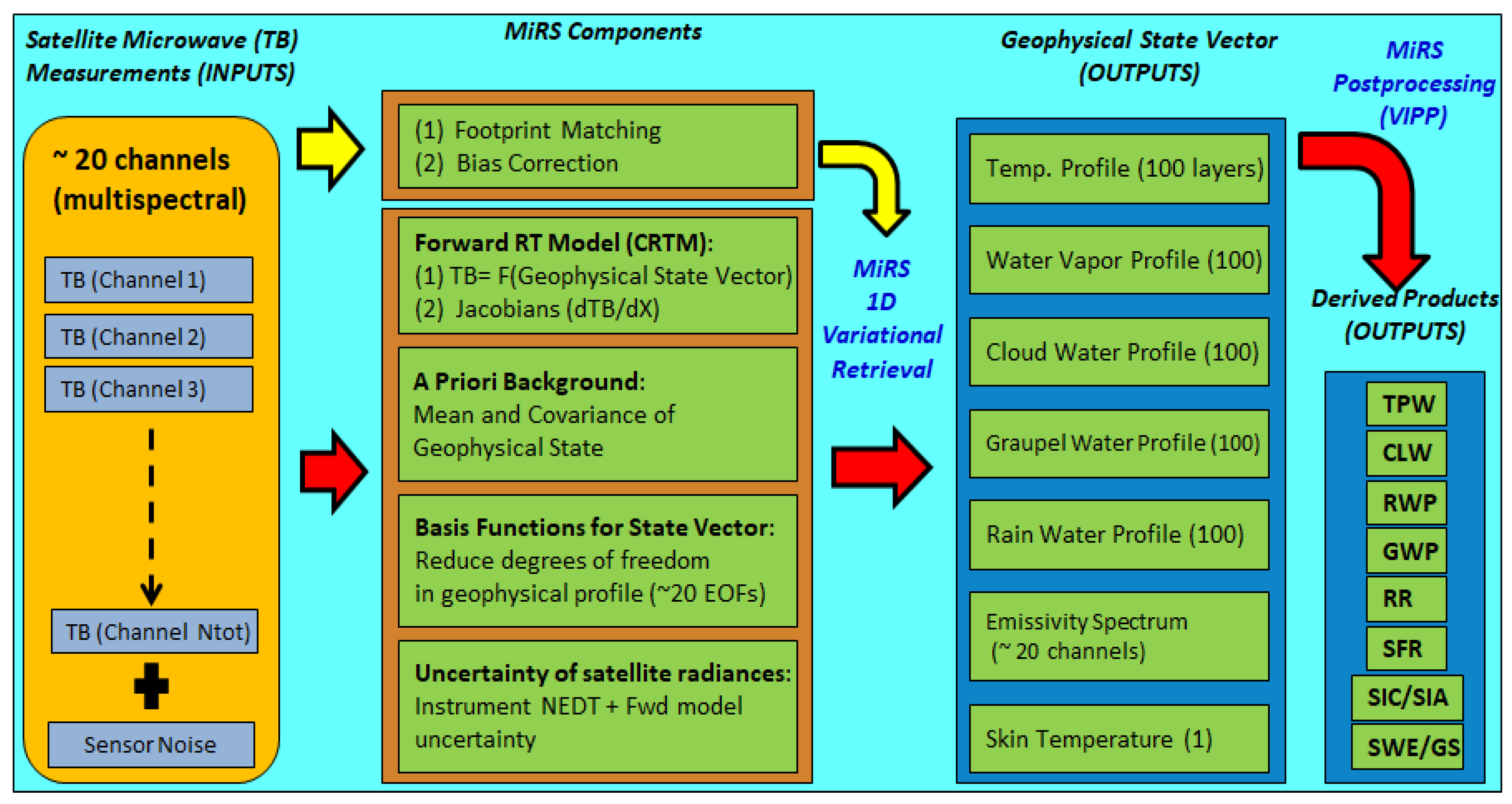
Figure 1. Schematic of MiRS processing components and data flow showing MiRS core retrieval and post-processing components. Core products are retrieved simultaneously as part of the state vector. Post-processing products are derived through vertical integration (water vapor, hydrometeors), catalogs (SIC, SWE), or fast regressions (rain rate). Post-processed hydrometeor retrieval products are Rain Rate, Graupel Water Path, Rain Water Path and Cloud Liquid Water.
Remotesensing 12 03160 g001
Figure 2. Global brightness temperature measurements minus simulations [K] over ocean, for 9 June 2019 at 31.4 GHz and 183.31 ± 7 GHz frequencies (a,c), and similarly for 1 October 2019 (b,d).
Remotesensing 12 03160 g002
Figure 3. Mean brightness temperature bias [K] of the 22 SNPP/ATMS channels over ocean with latitude between 55S and 55N for the true values (blue bars), NN prediction (orange bars) and their difference (red line). 1 October 2019.
Remotesensing 12 03160 g003
Figure 4. Brightness temperature bias [K] maps of SNPP/ATMS 23.8 GHz on 1 October 2019, over ocean with latitude between 55 S and 55 N, for (a) true value, (b) NN prediction, the difference between NN and the true value (c), and histograms of the true value and the NN prediction (d).
Remotesensing 12 03160 g004
Figure 5. MiRS temperature profiles (K) validated with ECMWF analyses for SNPP/ATMS over ocean for (a) clear, (b) cloudy, and (c) heavy cloud or light rain conditions on 1 October 2019. The black lines are for MiRS using the static bias correction method, and red for the NN bias correction method. Solid lines are for bias, and dashed lines for standard deviation.
Remotesensing 12 03160 g005
Figure 6. Similar to Figure 5 but for water vapor profiles. Bias and standard deviation are the percentage mixing ratio with respect to the mean ECMWF analysis at each layer.
Remotesensing 12 03160 g006
Figure 7. Total precipitable water (mm) of SNPP/ATMS on 1 October 2019, ascending node over ocean for (a) ECMWF analysis, (b) MiRS retrieval difference with ECMWF using static bias correction, (d) MiRS retrieval difference with ECMWF using NN bias correction, and (c) histograms of ECMWF and MiRS retrieval experiments shown in (a), (b), and (d).
Remotesensing 12 03160 g007
Figure 8. MiRS total precipitable water (mm) local zenith angle dependence of SNPP/ATMS on 1 October 2019 over ocean, ascending node. The black line is the result using a static bias correction and red line is the result using the NN bias correction.
Remotesensing 12 03160 g008
Figure 9. Skin temperature (K) scatterplots of SNPP/ATMS validated with ECMWF on 1 October 2019 over ocean, with ascending (top) and descending (bottom) nodes, using static (left) or NN (right) bias correction. The x-axis is MiRS skin temperature, and the y-axis represents ECMWF. The scatterplots are colored by the density of points.
Remotesensing 12 03160 g009
Table 1. Channel Characteristics of ATMS.
ChannelCentral Frequency
(GHz)
PolarizationBeam Width
(deg)
NEΔT
(K)
Peak WF (hPa)
123.8V5.20.9Window
231.4V5.20.9Window
350.3 H2.21.2Window
451.76 H2.20.75950
552.8 H2.20.75850
653.596 ± 0.115 H2.20.75700
754.4 H2.20.75400
854.94 H2.20.75250
955.5 H2.20.75200
1057.290344 H2.20.75100
1157.290344 ± 0.217 H2.21.250
1257.290344 ± 0.322 ± 0.048 H2.21.225
1357.290344 ± 0.322 ± 0.022 H2.21.510
1457.290344 ± 0.322 ± 0.010 H2.22.45
1557.290344 ± 0.322 ± 0.0045 H2.23.62
1688.2V2.20.5Window
17165.5 H1.10.6Window
18183.31 ± 7.0 H1.10.8800
19183.31 ± 4.5 H1.10.8700
20183.31 ± 3.0 H1.10.8500
21183.31 ± 1.8 H1.10.8400
22183.31 ± 1.0 H1.10.9300
Table 2. Days Used for NN Training.
14-January-201915-July-2018
15-February-20191-August-2018
25-March-20191-September-2019
1-April-201920-October-2018
11-May-20191-November-2019
4-June-20191-December-2019
Table 3. Performance metrics of MiRS retrievals including TPW, Tskin, emissivity (EM) at 23.8 GHz and 88.2 GHz, validated using ECMWF analyses (and FASTEM5 for emissivity) for SNPP/ATMS 1 October 2019 over ocean, ascending node. The numbers inside parentheses are sample sizes. The bias change percentages refer to their magnitude changes.
TPW
(mm)
Static
(868,412)
NN
(875,423)
Change (%)EM 23.8 GHzStatic
(868,299)
NN
(875,351)
Change (%)
Correlation0.990.990%Correlation0.58620.6740+15.0%
Bias1.520.60−60.5%Bias0.00710.0099+42.9%
Std. Dev2.332.62+12.9%Std. Dev0.03530.0255−25.7%
Tskin
(K)
Static
(868,299)
NN
(875,351)
Change (%)EM
88.2 GHz
Static
(868,299)
NN
(875,351)
Change (%)
Correlation0.960.97+1.0%Correlation0.71350.7229+1.3%
Bias0.38−0.05−86.8%Bias0.0022−0.0004−80.0%
Std. Dev3.013.02+0.3%Std. Dev0.03110.0301−3.2%