GPM-Based Multitemporal Weighted Precipitation Analysis Using GPM_IMERGDF Product and ASTER DEM in EDBF Algorithm

To obtain the high-resolution multitemporal precipitation using spatial downscaling technique on a precipitation dataset may provide a better representation of the spatial variability of precipitation to be used for different purposes. In this research, a new downscaling methodology such as the global precipitation mission (GPM)-based multitemporal weighted precipitation analysis (GMWPA) at 0.05° resolution is developed and applied in the humid region of Mainland China by employing the GPM dataset at 0.1° and the Advanced Spaceborne Thermal Emission and Reflection Radiometer (ASTER) 30 m DEM-based geospatial predictors, i.e., elevation, longitude, and latitude in empirical distribution-based framework (EDBF) algorithm. The proposed methodology is a two-stepped process in which a scale-dependent regression analysis between each individual precipitation variable and the EDBF-based weighted precipitation with geospatial predictor(s), and to downscale the predicted multitemporal weighted precipitation at a refined scale is developed for the downscaling of GMWPA. While comparing results, it shows that the weighted precipitation outperformed all precipitation variables in terms of the coefficient of determination (R²) value, whereas they outperformed the annual precipitation variables and underperformed as compared to the seasonal and the monthly variables in terms of the calculated root mean square error (RMSE) value. 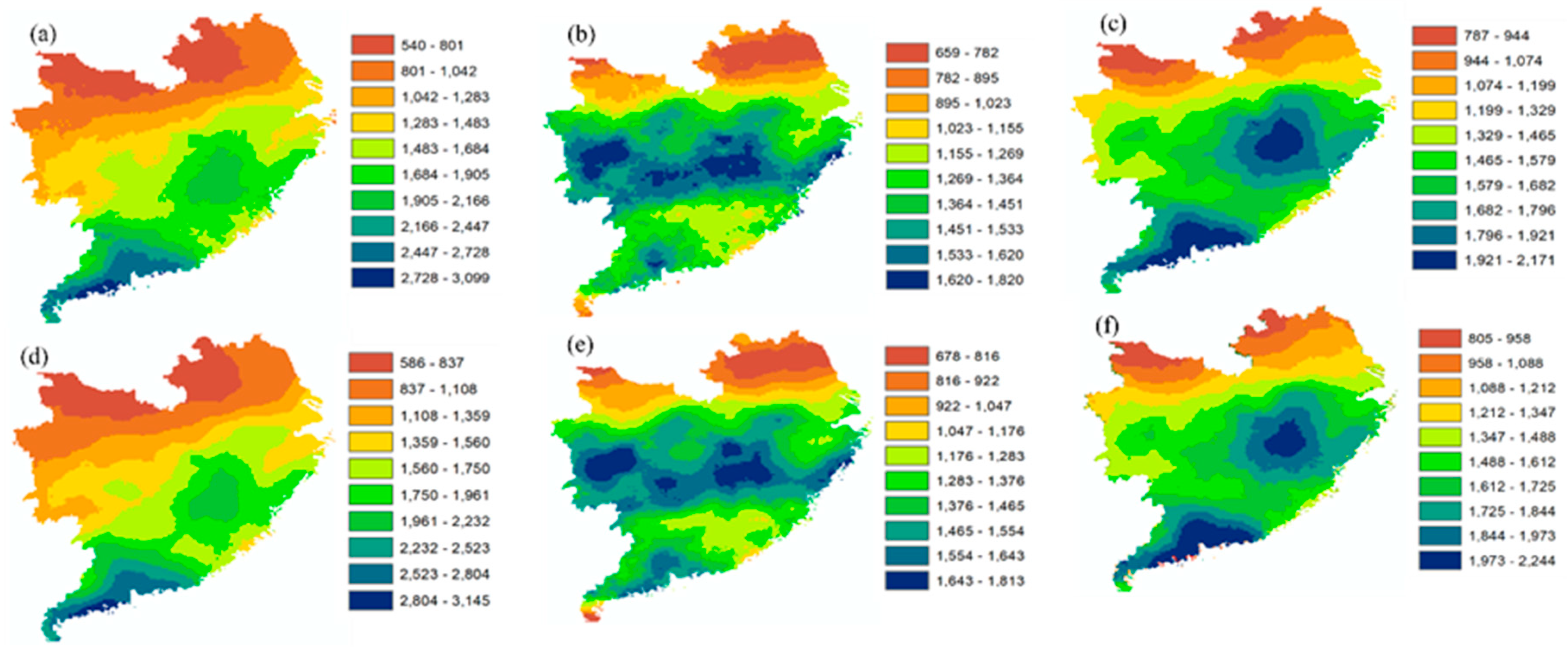Based on the achieved results, the weighted precipitation at the low-resolution (e.g., at 0.75° resolution) along-with the original resolution (e.g., at 0.1° resolution) is employed in the downscaling process to predict the average multitemporal precipitation, the annual total precipitation for the year 2001 and 2004, and the average annual precipitation (2001–2015) at 0.05° resolution, respectively. The downscaling approach resulting through proposed methodology captured the spatial patterns with greater accuracy at higher spatial resolution. This work showed that it is feasible to increase the spatial resolution of a precipitation variable(s) with greater accuracy on an annual basis or as an average from the multitemporal precipitation dataset using a geospatial predictor as the proxy of precipitation through the weighted precipitation in EDBF environment.

References

- Langella, G.; Basile, A.; Bonfante, A.; Terribile, F. High-resolution space–time rainfall analysis using integrated ANN inference systems. J. Hydrol. 2010, 387, 328–342. [Google Scholar] [CrossRef]
- Lopez, P.; Immerzeel, W.; Rodríguez Sandoval, E.; Sterk, G.; Schellekens, J. Spatial downscaling of satellite-based precipitation and its impact on discharge simulations in the Magdalena River Basin in Clombia. Front. Earth Sci. 2018, 6, 68. [Google Scholar] [CrossRef]
- Jia, S.; Zhu, W.; Lu, A.; Yan, T. A statistical spatial downscaling algorithm of TRMM precipitation based on NDVI and DEM in the Qaidam Basin of China. Remote Sens. Environ. 2011, 115, 3069–3079. [Google Scholar] [CrossRef]
- Li, M.; Shao, Q. An improved statistical approach to merge satellite rainfall estimates and rain gauge data. J. Hydrol. 2010, 385, 51–64. [Google Scholar] [CrossRef]
- Goodrich, D.; Faurès, J.; Woolhiser, D.; Lane, L.; Sorooshian, S. Measurement and analysis of small-scale convective storm rainfall variability. J. Hydrol. 1995, 173, 283–308. [Google Scholar] [CrossRef]
- Wheater, H.; Isham, V.; Cox, D.; Chandler, R.; Kakou, A.; Northrop, P.; Oh, L.; Onof, C.; Rodriguez-Iturbe, I. Spatial-temporal rainfall fields: Modelling and statistical aspects. Hydrol. Earth Syst. Sci. 2000, 4, 581–601. [Google Scholar] [CrossRef]
- Gruber, A.; Levizzani, V. Assessment of global precipitation products: A project of the World Climate Research Programmed Global Energy and Water Cycle Experiment (GEWEX) Radiation Panel; WCRP-128; WMO: Geneva, Switzerland, 2008; p. 50. [Google Scholar]
- Wilheit, T. Some comments on passive microwave measurement of rain. Bull. Am. Meteorol. Soc. 1986, 67, 1226–1232. [Google Scholar] [CrossRef]
- Loukas, A.; Vasiliades, L. Streamflow simulation methods for ungauged and poorly gauged watersheds. Nat. Hazard Earth Syst. Sci. 2014, 14, 1641. [Google Scholar] [CrossRef]
- Sivapalan, M.; Takeuchi, K.; Franks, S.; Gupta, V.; Karambiri, H.; Lakshmi, V.; Liang, X.; McDonnell, J.; Mendiondo, E.; O’connell, P. IAHS decade on Predictions in Ungauged Basins (PUB), 2003–2012: Shaping an exciting future for the hydrological sciences. Hydrol. Sci. J. 2010, 48, 857–880. [Google Scholar] [CrossRef]
- Beesley, C.; Frost, A.; Zajaczkowski, J. A comparison of the BAWAP and SILO spatially interpolated daily rainfall datasets. In Proceedings of the 18th World IMACS/MODSIM Congress, Cairns, Australia, 13–17 July 2009. [Google Scholar]
- Hughes, D. Comparison of satellite rainfall data with observations from gauging station networks. J. Hydrol. 2006, 327, 399–410. [Google Scholar]
- Jeffery, S. Error Analysis for the interpolation of monthly rainfall used in the generation of SILO rainfall datasets; Technical Report; The Queensland Department of Natural Resources: Brisbane City, Australia, 2006. [Google Scholar]
- Collischonn, B.; Collischonn, W.; Tucci, C.E.M. Daily hydrological modeling in the Amazon basin using TRMM rainfall estimates. J. Hydrol. 2008, 360, 207–216. [Google Scholar] [CrossRef]
- Bohnenstengel, S.I.; Schlünzen, K.; Beyrich, F. Representativity of in situ precipitation measurements–A case study for the LITFASS area in North-Eastern Germany. J. Hydrol. 2011, 400, 387–395. [Google Scholar] [CrossRef]
- Dingman, S. Physical Hydrology; Prentice Hall: New Jersey, NJ, USA, 2002. [Google Scholar]
- Michaelides, S.; Levizzani, V.; Anagnostou, E.; Bauer, P.; Kasparis, T.; Lane, J. Precipitation: Measurement, remote sensing, climatology and modeling. Atmos. Res. 2009, 94, 512–533. [Google Scholar] [CrossRef]
- Nastos, P.; Kapsomenakis, J.; Philandras, K. Evaluation of the TRMM 3B43 gridded precipitation estimates over Greece. Atmos. Res. 2016, 169, 497–514. [Google Scholar] [CrossRef]
- Adler, R.; Kidd, C.; Petty, G.; Morissey, M.; Goodman, H. Inter-comparison of global precipitation products: The third Precipitation Inter-comparison Project (PIP-3). Bull. Am. Meteorol. Soc. 2001, 82, 1377–1396. [Google Scholar]
- Huffman, G.; Adler, R.; Arkin, P.; Chang, A.; Ferraro, R.; Gruber, A.; Janowiak, J.; McNab, A.; Rudolf, B.; Schneider, U. The global precipitation climatology project (GPCP) combined precipitation dataset. Bull. Am. Meteorol. Soc. 1997, 78, 5–20. [Google Scholar] [CrossRef]
- Huffman, G.; Adler, R.; Morrissey, M.; Bolvin, D.; Curtis, S.; Joyce, R.; McGavock, B.; Susskind, J. Global precipitation at one-degree daily resolution from multisatellite observations. J. Hydrometeorol. 2001, 2, 36–50. [Google Scholar] [CrossRef]
- Huffman, G.; Adler, R.; Bolvin, D.; Gu, G. Improving the global precipitation record: GPCP version 2.1. Geophys. Res. Lett. 2009, 36. [Google Scholar] [CrossRef]
- Kubota, T.; Shige, S.; Hashizume, H.; Aonashi, K.; Takahashi, N.; Seto, S.; Hirose, M.; Takayabu, Y.; Ushio, T.; Nakagawa, K. Global precipitation map using satellite-borne microwave radiometers by the GSMaP project: Production and validation. IEEE Trans. Geosci. Remote Sens. Environ. 2007, 45, 2259–2275. [Google Scholar] [CrossRef]
- Beck, H.; Van Dijk, A.; Levizzani, V.; Schellekens, J.; Gonzalez Miralles, D.; Martens, B.; De Roo, A. MSWEP: 3-hourly 0.25 global gridded precipitation (1979–2015) by merging gauge, satellite, and reanalysis data. Hydrol. Earth Syst. Sci. 2017, 21, 589–615. [Google Scholar] [CrossRef]
- Funk, C.; Peterson, P.; Landsfeld, M.; Pedreros, D.; Verdin, J.; Shukla, S.; Husak, G.; Rowland, J.; Harrison, L.; Hoell, A. The climate hazards infrared precipitation with stations—A new environmental record for monitoring extremes. Sci. Data 2015, 2, 1–21. [Google Scholar] [CrossRef]
- Hsu, K.-L.; Gao, X.; Sorooshian, S.; Gupta, H. Precipitation estimation from remotely sensed information using artificial neural networks. J. Appl. Meteorol. 1997, 36, 1176–1190. [Google Scholar] [CrossRef]
- Kummerow, C.; Barnes, W.; Kozu, T.; Shiue, J.; Simpson, J. The tropical rainfall measuring mission (TRMM) sensor package. J. Atmos. Ocean. Technol. 1998, 15, 809–817. [Google Scholar] [CrossRef]
- Kummerow, C.; Simpson, J.; Thiele, O.; Barnes, W.; Chang, A.; Stocker, E.; Adler, R.; Hou, A.; Kakar, R.; Wentz, F. The status of the Tropical Rainfall Measuring Mission (TRMM) after two years in orbit. J. Appl. Meteorol. 2000, 39, 1965–1982. [Google Scholar] [CrossRef]
- Huffman, G.; Bolvin, D.; Nelkin, E.; Wolff, D.; Adler, R.; Gu, G.; Hong, Y.; Bowman, K.; Stocker, E. The TRMM multisatellite precipitation analysis (TMPA): Quasi-global, multiyear, combined-sensor precipitation estimates at fine scales. J. Hydrometeorol. 2007, 8, 38–55. [Google Scholar] [CrossRef]
- Ma, Z.; Shi, Z.; Zhou, Y.; Xu, J.; Yu, W.; Yang, Y. A spatial data mining algorithm for downscaling TMPA 3B43 V7 data over the Qinghai–Tibet Plateau with the effects of systematic anomalies removed. Remote Sens. Environ. 2017, 200, 378–395. [Google Scholar] [CrossRef]
- Mahmud, M.; Mohd Yusof, A.; Mohd Reba, M.; Hashim, M. Mapping the daily rainfall over an ungauged tropical micro-watershed: A downscaling algorithm using GPM data. Water 2020, 12, 1661. [Google Scholar]
- Hou, A.; Kakar, R.; Neeck, S.; Azarbarzin, A.; Kummerow, C.; Kojima, M.; Oki, R.; Nakamura, K.; Iguchi, T. The global precipitation measurement mission. Bull. Am. Meteorol. Soc. 2014, 95, 701–722. [Google Scholar] [CrossRef]
- Huffman, G.; Stocker, E.; Bolvin, D.; Nelkin, E.; Tan, J. GPM IMERG Final Precipitation L3 1 day 0.1 degree × 0.1 degree V06. In Goddard Earth Sciences Data and Information Services Center (GES DISC); Andrey, G., Savtchenko, M.D., Eds.; NASA: Washington, DC, USA, 2019. [Google Scholar]
- Duan, Z.; Bastiaanssen, W. First results from Version 7 TRMM 3B43 precipitation product in combination with a new downscaling–calibration procedure. Remote Sens. Environ. 2013, 131, 1–13. [Google Scholar] [CrossRef]
- Hunink, J.; Immerzeel, W.; Droogers, P. A High-resolution Precipitation 2-step mapping Procedure (HiP2P): Development and application to a tropical mountainous area. Remote Sens. Environ. 2014, 140, 179–188. [Google Scholar] [CrossRef]
- Zhang, Q.; Shi, P.; Singh, V.; Fan, K.; Huang, J. Spatial downscaling of TRMM-based precipitation data using vegetative response in Xinjiang, China. Int. J. Climatol. 2017, 37, 3895–3909. [Google Scholar] [CrossRef]
- Ulloa, J.; Ballari, D.; Campozano, L.; Samaniego, E. Two-step downscaling of TRMM 3B43 V7 precipitation in contrasting climatic regions with sparse monitoring: The case of Ecuador in Tropical South America. Remote Sens. 2017, 9, 758. [Google Scholar] [CrossRef]
- Shi, Y.; Song, L.; Xia, Z.; Lin, Y.; Myneni, R.; Choi, S.; Wang, L.; Ni, X.; Lao, C.; Yang, F. Mapping annual precipitation across Mainland China in the period 2001–2010 from TRMM 3B43 product using spatial downscaling approach. Remote Sens. 2015, 7, 5849–5878. [Google Scholar] [CrossRef]
- Immerzeel, W.; Rutten, M.; Droogers, P. Spatial downscaling of TRMM precipitation using vegetative response on the Iberian Peninsula. Remote Sens. Environ. 2009, 113, 362–370. [Google Scholar] [CrossRef]
- Chen, F.; Liu, Y.; Liu, Q.; Li, X. Spatial downscaling of TRMM 3B43 precipitation considering spatial heterogeneity. Int. J. Remote Sens. 2014, 35, 3074–3093. [Google Scholar] [CrossRef]
- Alexakis, D.; Tsanis, I. Comparison of multiple linear regression and artificial neural network models for downscaling TRMM precipitation products using MODIS data. Environ. Earth Sci. 2016, 75, 1077. [Google Scholar] [CrossRef]
- Ceccherini, G.; Ameztoy, I.; Hernández, C.; Moreno, C. High-resolution precipitation datasets in South America and West Africa based on satellite-derived rainfall, enhanced vegetation index and digital elevation model. Remote Sens. 2015, 7, 6454–6488. [Google Scholar] [CrossRef]
- Goovaerts, P. Geostatistical approaches for incorporating elevation into the spatial interpolation of rainfall. J. Hydrol. 2000, 228, 113–129. [Google Scholar] [CrossRef]
- Zhang, Y.; Li, Y.; Ji, X.; Luo, X.; Li, X. Fine-resolution precipitation mapping in a mountainous watershed: Geostatistical downscaling of TRMM products based on environmental variables. Remote Sens. 2018, 10, 119. [Google Scholar] [CrossRef]
- Fang, J.; Du, J.; Xu, W.; Shi, P.; Li, M.; Ming, X. Spatial downscaling of TRMM precipitation data based on the orographical effect and meteorological conditions in a mountainous area. Adv. Water Resour. 2013, 61, 42–50. [Google Scholar] [CrossRef]
- Park, N. Spatial downscaling of TRMM precipitation using geostatistics and fine scale environmental variables. Adv. Meteorol. 2013, 2013, 237126. [Google Scholar] [CrossRef]
- Chen, C.; Zhao, S.; Duan, Z.; Qin, Z. An improved spatial downscaling procedure for TRMM 3B43 precipitation product using geographically weighted regression. IEEE J. Sel. Top. Appl. Earth Obs. Remote Sens. 2015, 8, 4592–4604. [Google Scholar] [CrossRef]
- Xu, G.; Xu, X.; Liu, M.; Sun, A.; Wang, K. Spatial downscaling of TRMM precipitation product using a combined multifractal and regression approach: Demonstration for South China. Water 2015, 7, 3083–3102. [Google Scholar] [CrossRef]
- Ezzine, H.; Bouziane, A.; Ouazar, D.; Hasnaoui, M. Downscaling of open coarse precipitation data through spatial and statistical analysis, integrating NDVI, NDWI, ELEVATION, and distance from sea. Adv. Meteorol. 2017, 2017, 8124962. [Google Scholar] [CrossRef]
- Xu, S.; Wu, C.; Wang, L.; Gonsamo, A.; Shen, Y.; Niu, Z. A new satellite-based monthly precipitation downscaling algorithm with non-stationary relationship between precipitation and land surface characteristics. Remote Sens. Environ. 2015, 162, 119–140. [Google Scholar] [CrossRef]
- Mitas, L.; Mitasova, H. General variational approach to the interpolation problem. Comput. Math. Appl. 1988, 16, 983–992. [Google Scholar] [CrossRef]
- Li, S.; Yang, S.; Liu, X. Spatiotemporal variability of extreme precipitation in north and south of the Qinling-Huaihe region and influencing factors during 1960–2013. Prog. Geogr. 2015, 34, 354–363. [Google Scholar]
- NASA; METI; AIST; Japan Space System. ASTER Global Digital Elevation Model V003. NASA EOSDIS Land Processes DAAC. 2019. Available online: https://cmr.earthdata.nasa.gov/search/concepts/C1299783579-LPDAAC_ECS.html (accessed on 20 June 2020).
- Ullah, S.; Farooq, M.; Sarwar, T.; Tareen, M.J.; Wahid, M.A. Flood modeling and simulations using hydrodynamic model and ASTER DEM—A case study of Kalpani River. Arab. J. Geosci. 2016, 9, 439. [Google Scholar] [CrossRef]
- Huffman, G.; Adler, R.; Bolvin, D.; Nelkin, E. The TRMM Multi-satellite Precipitation Analysis (TMPA), in Chapter 1. In Satellite Rainfall Applications for Surface Hydrology; Springer: Dordrecht, The Netherlands, 2010. [Google Scholar]
- Miller, R.; Siegmund, D. Maximally selected Chi-square statistics. Biometrics 1982, 38, 1101–1106. [Google Scholar] [CrossRef]
- Ahn, C.W.; Ramakrishna, R.S. Elitism-based compact genetic algorithms. IEEE Trans. Evol. Comput. 2003, 4, 367–385. [Google Scholar]
- Zuo, Z.; Yan, L.; Ullah, S.; Sun, S.; Zhang, R.; Zhao, H. Empirical distribution based framework for improving multi-parent crossover algorithms. Soft Comput. 2020, in press. [Google Scholar]
- Verlinde, J. TRMM Rainfall Data Downscaling in the Pangani Basin in Tanzania; Delft University of Technology: Delft, The Netherlands, 2011. [Google Scholar]
- Franke, R. Smooth interpolation of scattered data by local thin plate splines. Comput. Math. Appl. 1982, 8, 237–281. [Google Scholar] [CrossRef]
- Eiben, A.E.; Back, T. Empirical investigation of multiparent recombination operators in evolution strategies. Evol. Comput. 1997, 5, 347–365. [Google Scholar] [CrossRef] [PubMed]
- Herrera, F.; Lozano, M.; Verdegay, J.L. Tackling real-coded genetic algorithms: Operators and tools for behavioral analysis. Artif. Intell. Rev. 1998, 12, 265–319. [Google Scholar] [CrossRef]
- Goldberg, D.E. Real-coded genetic algorithms, virtual alphabets, and blocking. Complex Syst. 1991, 5, 139–167. [Google Scholar]
- Agam, N.; Kustas, W.P.; Anderson, M.C.; Li, F.; Neale, C.M.U. A vegetation index based 572 technique for spatial sharpening of thermal imagery. Remote Sens. Environ. 2007, 107, 545–558. [Google Scholar] [CrossRef]