Article

Combining Multi-Sensor Satellite Imagery to Improve Long-Term Monitoring of Temporary Surface Water Bodies in the Senegal River Floodplain

1
G-EAU, AgroParisTech, Cirad, INRAE, IRD, Montpellier SupAgro, University of Montpellier, Montpellier 34196 CEDEX 5, France
2
ISRA, BAME, BP 3120 Dakar, Senegal
3
Leïdi Laboratory—Dynamics of Territories and Development, Gaston Berger University (UGB), BP 234 Saint-Louis, Senegal
4
Department of Geography, Cheikh Anta Diop University (UCAD), BP 5005 Dakar, Senegal
5
UFR S2ATA Agronomic Sciences, Aquaculture and Food Technologies, Gaston Berger University (UGB), BP 234 Saint-Louis, Senegal
6
Laboratory of Hydraulics and Fluid Mechanics, Faculty of Sciences and Techniques, Department of Physics, Cheikh Anta Diop University (UCAD), BP 5005 Dakar, Senegal
*
Author to whom correspondence should be addressed.
Remote Sens. 2020, 12(19), 3157; https://doi.org/10.3390/rs12193157
Submission received: 21 July 2020 / Revised: 4 September 2020 / Accepted: 14 September 2020 / Published: 26 September 2020
(This article belongs to the Special Issue Remote Sensing and Modeling of Land Surface Water)

Abstract

:
Accurate monitoring of surface water bodies is essential in numerous hydrological and agricultural applications. Combining imagery from multiple sensors can improve long-term monitoring; however, the benefits derived from each sensor and the methods to automate long-term water mapping must be better understood across varying periods and in heterogeneous water environments. All available observations from Landsat 7, Landsat 8, Sentinel-2 and MODIS over 1999–2019 are processed in Google Earth Engines to evaluate and compare the benefits of single and multi-sensor approaches in long-term water monitoring of temporary water bodies, against extensive ground truth data from the Senegal River floodplain. Otsu automatic thresholding is compared with default thresholds and site-specific calibrated thresholds to improve Modified Normalized Difference Water Index (MNDWI) classification accuracy. Otsu thresholding leads to the lowest Root Mean Squared Error (RMSE) and high overall accuracies on selected Sentinel-2 and Landsat 8 images, but performance declines when applied to long-term monitoring compared to default or site-specific thresholds. On MODIS imagery, calibrated thresholds are crucial to improve classification in heterogeneous water environments, and results highlight excellent accuracies even in small (19 km 2 ) water bodies despite the 500 m spatial resolution. Over 1999–2019, MODIS observations reduce average daily RMSE by 48% compared to the full Landsat 7 and 8 archive and by 51% compared to the published Global Surface Water datasets. Results reveal the need to integrate coarser MODIS observations in regional and global long-term surface water datasets, to accurately capture flood dynamics, overlooked by the full Landsat time series before 2013. From 2013, the Landsat 7 and Landsat 8 constellation becomes sufficient, and integrating MODIS observations degrades performance marginally. Combining Landsat and Sentinel-2 yields modest improvements after 2015. These results have important implications to guide the development of multi-sensor products and for applications across large wetlands and floodplains.

Graphical Abstract

1. Introduction

Accelerating climate and human changes have significant influences on hydrological systems and notably on surface water dynamics [1]. Accurate mapping and monitoring of lakes, reservoirs and wetlands is essential to understand inundation patterns, water availability for irrigation, domestic use or hydropower, as well as ecosystem health. Across large wetlands and multiple dispersed water bodies, remote sensing provides rising opportunities to monitor surface water variations, which can be difficult to capture by localised hydrological monitoring or modelling [2]. These notably face stark difficulties in representing flooded areas due to data scarcity and inaccuracies in global digital elevation models to represent and account for the flat, yet complex topography of large floodplains [3].
In recent years, several works have harnessed the rising number of free, high spatial and temporal resolution imagery from passive and active sensors, mapping and monitoring small water bodies [4,5,6,7], lakes, floodplains and wetlands [8,9,10,11,12,13,14]. In parallel, numerous surface water databases have been developed at the global and regional scale. The Moderate Resolution Imaging Spectroradiometer (MODIS) with up to twice daily observations from the Aqua and Terra constellation of sensors has notably been used in several land cover applications. Carroll et al. [15] produced a global inventory of surface water using MODIS and Shuttle Radar Topography Missions (SRTM) elevation data for the year 2000, updated by the 250 m Global Water Pack produced by Klein et al. [16]. Khandelwal et al. [17] developed an approach for global eight day monitoring of surface water extent using 500 m MODIS imagery, while D’Andrimont and Defourny [18] used twice daily observations to characterise surface water at a 10 day time step over 2004–2010 across Africa.
The multiplication of higher resolution sensors notably Landsat and Sentinel missions has led global-scale analyses to move towards moderate resolution [19]. Feng et al. [20], Verpoorter et al. [21] for instance produced a 30 m inland water body dataset for the year 2000 based on Landsat imagery. Yamazaki et al. [22] developed the Global 3 arc-second (90 m) Water Body Map (G3WBM) based on Landsat multi-temporal imagery and the Global Land Survey (GLS) database. Using the full catalogue of Landsat imagery, Pekel et al. [23] developed the Global Surface Water (GSW) dataset harnessing Google Earth Engines’ (GEE) [24] capacity to produce not only a global water map, but also a database of water dynamics over 1984 to 2019 at a 30 m spatial resolution and a monthly scale. This can notably be combined with satellite altimetry data (e.g., DAHITI [25]) to produce global lake and reservoir volume estimates. Donchyts et al. [26] produced a similar tool (Deltares Aqua Monitor) based on Landsat imagery at a 30 m resolution, while Yang et al. [27] recently used Level 1C Sentinel-2 imagery in GEE to map surface water dynamics across the whole of France.
Despite the vast opportunities provided by these global datasets, research has also shown the limitations of these works in specific contexts. Optical sensors such as those aboard Landsat satellites are affected by cloud cover, leading to incomplete representation of seasonal wetlands and inundation patterns [28]. To overcome these limitations, Yao et al. [29] used Landsat imagery since 1992 and enhanced cloud corrections to increase the number of available observations and create a long-term high frequency time series. Based on multiple sensors, including active sensors, a global database of surface water extent over 12 years (Global Inundation Extent from Multi-Satellites—GIEMS) was developed at a 0.25 (around 27 km) resolution, subsequently downscaled to 500 m based on ancillary data [30,31,32]. Combining optical and radar imagery can notably improve observations during the rainy season when cloud obstructions interfere with reflectance values of passive sensors [33]. Similarly, a rising number of works seek to combine the unparalleled long-term observations from Landsat (launched in 1972) with the recent advances from Sentinel-2 imagery [34,35], and NASA has distributed Harmonized Landsat and Sentinel-2 surface reflectance datasets at a 30 m resolution since 2013 [36]. However, these approaches notably suffer from the difficulties associated with the presence of vegetation within the pixel affecting the spectral signature. Methods are indeed calibrated and designed to classify open water bodies, leading to omission errors on smaller water bodies, floodplains and wetlands containing large areas with flooded vegetation [22,23,28,37,38].
In mixed water environments such as floodplains, which concentrate meanders and shallow water basins and where temporary flood patterns require high image availability, novel approaches to build upon the multiple sources of imagery are necessary [39,40,41]. Optimal approaches to characterise long-term surface water extent must seek to combine or fuse the observations from multiple sensors [28,42]. Large-scale computing geoprocessing capacities made available through Google Earth Engines have vastly increased the possibilities to exploit multiple imagery across multiple locations. However, combining and fusing satellite sources require understanding the relative benefits of these observations including in long-term studies to guide their selection and combination [43,44]. The need for consistent long-term datasets to monitor land use also introduces further constraints to classify data and threshold indices in automated, but consistent ways [42,45,46], whose accuracy must be assessed and optimised against ground truth data.
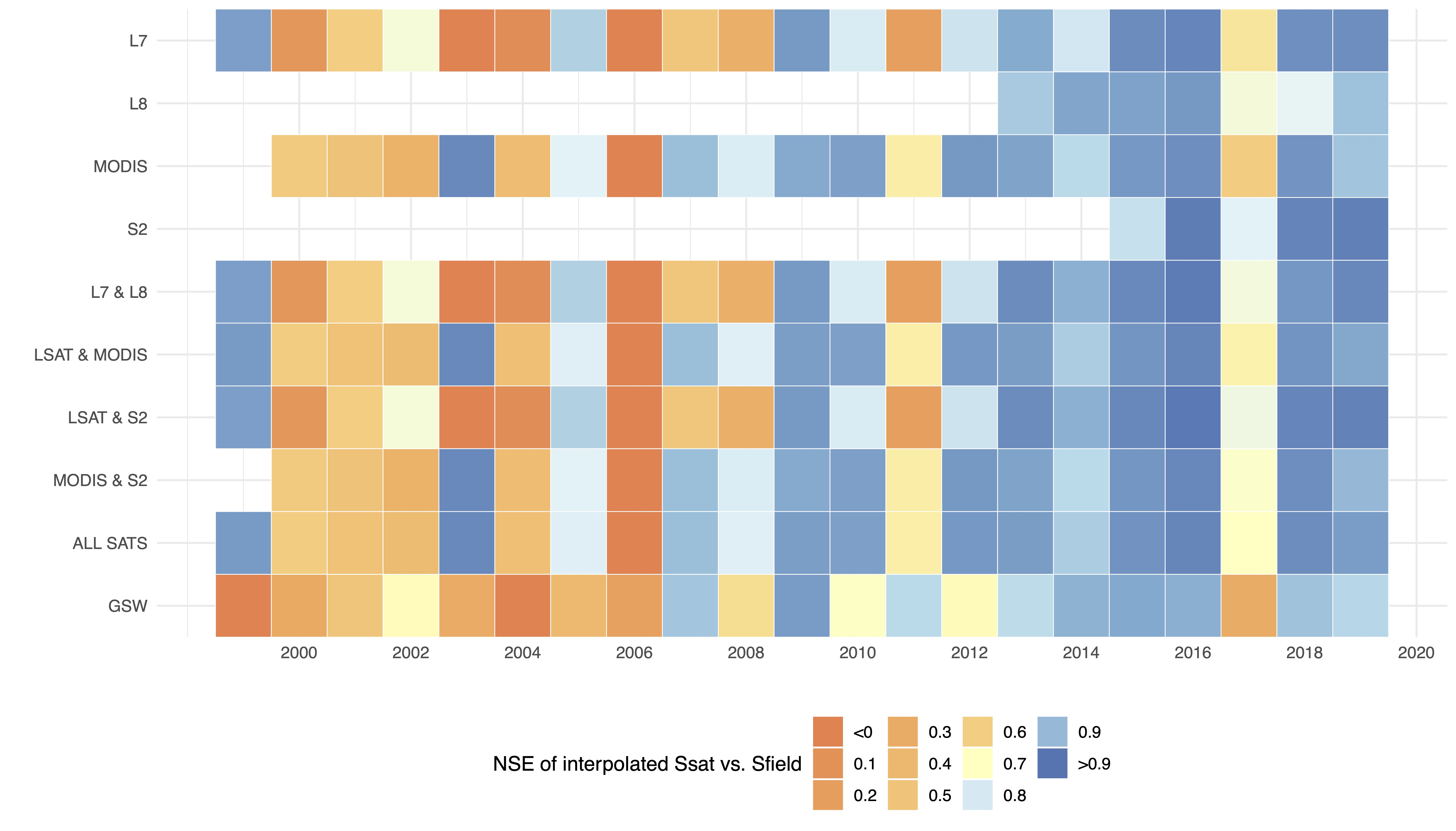
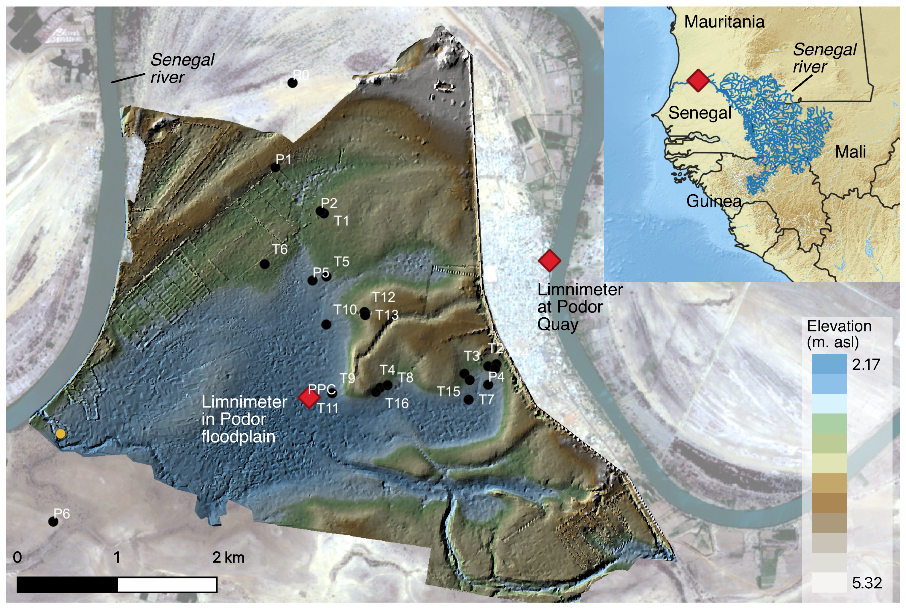
This paper seeks to evaluate and compare the relative benefits of combining multiple imagery sources to monitor surface water areas in floodplains, characterised by temporary inundation and heterogeneous water environments. Extensive and high accuracy field monitoring of surface water over 1999–2019 in the Senegal River floodplain is used to quantify the capacity and accuracy of four major sources of Earth observation to monitor long-term surface water variations. Three thresholding methods are compared to improve the classification of mixed waters with Landsat 7, Landsat 8, Sentinel-2 and MODIS, before associating all 1600 observations over 1999–2019 to evaluate the skill of single sensor and multi-sensor combinations and guide the development of long-term studies of large floodplains and wetlands. The possibilities offered within Google Earth Engines are explored in order to reduce downloading and processing times and easily replicate the approach and findings across entire floodplains of the large rivers of the world.
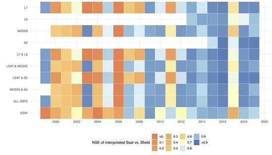
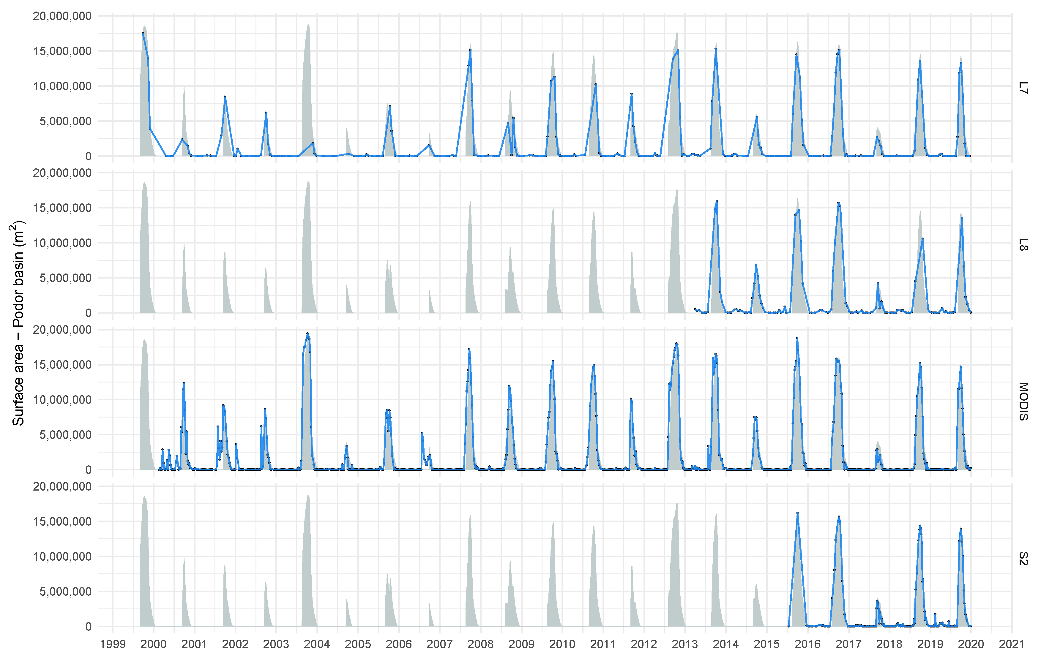
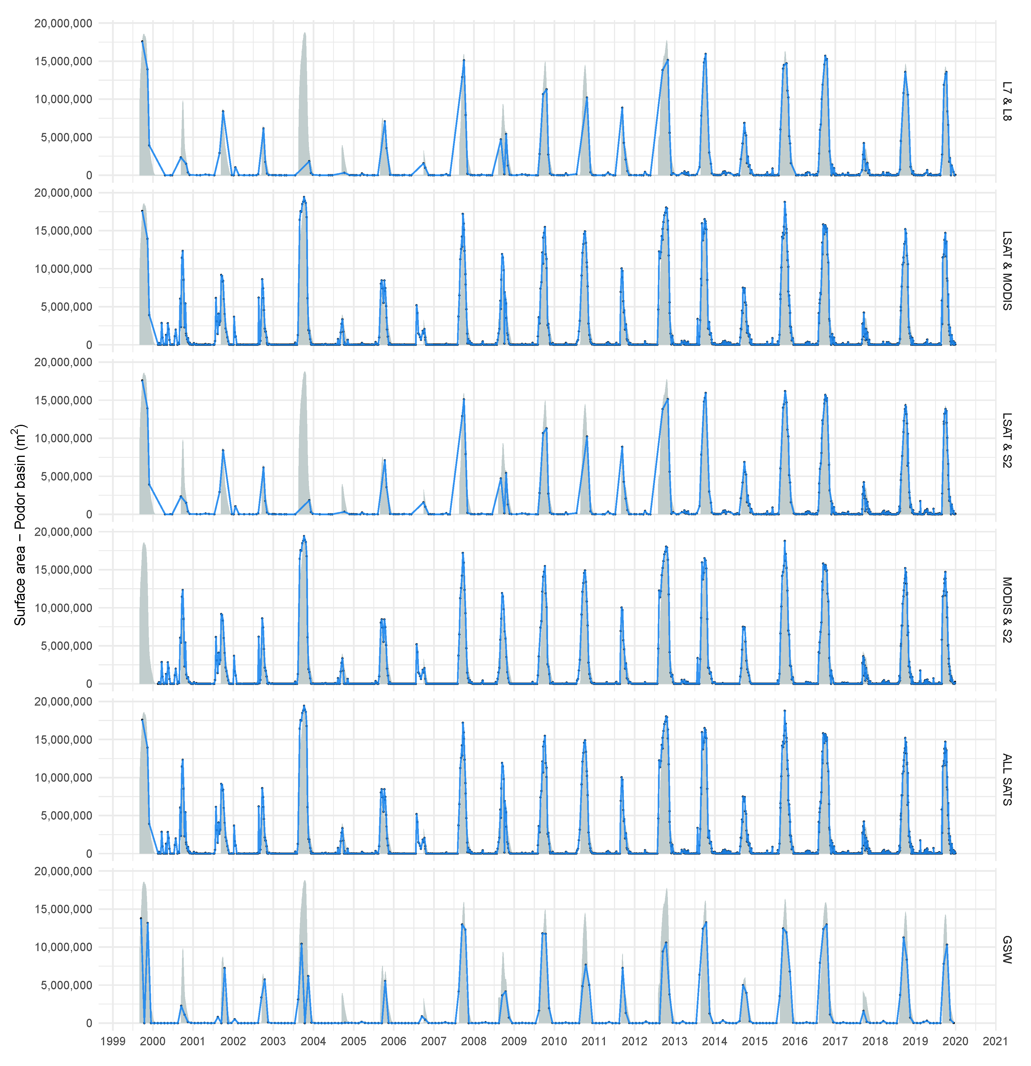
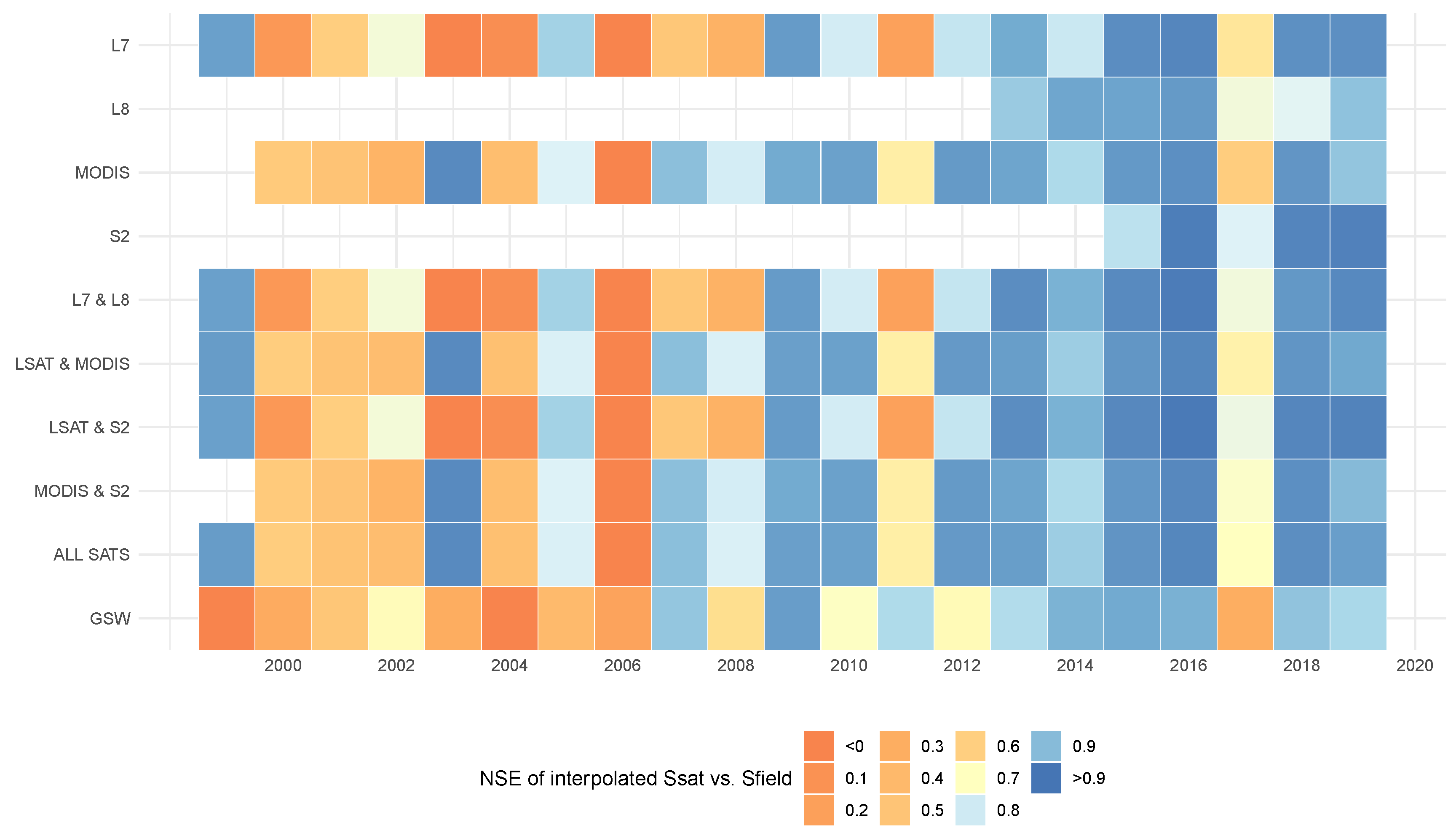
2. Materials and Methods

2.1. Case Study

Our research focusses on the alluvial floodplain of the Senegal River (1750 km), the second longest river in West Africa (Figure 1). The floodplain (2250 km 2 ) is composed of natural wetlands and irrigated perimeters and is extremely flat (slopes < 1%), with slight depressions that form tributaries and temporary water bodies. Located in the Sahelian climatic zone, these floodplains are mainly fed by the heavy rainfall during the West African monsoon over an upstream Guinean basin, which generates a peak flood in September–October. These floods are sources of wealth for fishermen, herders and hunters and exploited for rice and sorghum cultivation in traditional free flooding irrigation systems, and as a result are the focus of research on agronomic, hydrological and social issues. The Podor depression (19 km 2 ), situated in the extreme north of Senegal, 180 km from Saint-Louis, is a representative site of the Senegal River floodplain and has been the subject of ongoing research to explore socio-hydrological dynamics [47,48]. Mapping and characterising the flood patterns in the floodplain is important to understand agricultural and socio-economic practices, as well as the influence of climatic and human changes in the upstream catchments. Ongoing research provides a long-term time series of hydrological observations, as well as substantial ground truth data. These are exploited here to compare and assess the accuracy of remote sensing approaches and guide the extrapolation of optimal methods and findings across the entire floodplain of large rivers. The data mobilised in this research are presented in detail in the following subsections and summarised in Figure 2.

2.2. Satellite Imagery

2.2.1. Landsat Data

Three-hundred one images from the ETM+ sensor aboard the Landsat 7 satellite and 151 images from OLI sensor on Landsat 8 were used in this study. These sensors have similar characteristics providing multispectral imagery at 30 m spatial resolution, at a 16 day time interval (Table 1). The combination of imagery from Landsat 7 and Landsat 8 satellites can reduce repetitivity to eight days after 2013 thanks to the eight day offset between their acquisitions [49]. Landsat 5 launched in 1984 was not used here. For our region of interest, image availability is extremely low, with only 100 images acquired between 3 May 1984 and the last observation on 21 October 2011. Over the period considered here, 1999–2019, only 38 Landsat 5 TM images are available for this region (Figure A1), unequally distributed over time as 16 of these are for the year 2007 and before the flood. Tiles from path 204 and row 49 were used here. Our region of interest overlaps on row 48; however, there is no benefit from combining both observations as rows are captured in close succession. The minor delay between rows 48 and 49 can change cloud presence, but only marginally, as observed here. Where the region of interest overlaps on two paths, this can result in a greater frequency of observations [7].
Images provided by the U.S. Geological Survey (USGS) ESPA are processed to surface reflectance (Level 2A) using the Landsat Ecosystem Disturbance Adaptive Processing System (LEDAPS) for sensors TM and ETM+ and the Landsat Surface Reflectance Code (LaSRC) for the OLI sensor. These surface reflectance products are available directly from USGS data centres such as Earth Explorer and through Google Earth Engines (assets LANDSAT/LE07/C01/T1_SR and LANDSAT/LC08/C01/T1_SR).

2.2.2. MODIS Data

Nine-hundred thirteen images from the MODIS sensor aboard the Terra satellite were used. With its wide swath, this medium resolution sensor benefits from shorter recurrence periods and provides daily coverage of many parts of the globe. Multispectral imagery is captured at 250 m in 2 bands, 500 m in 5 bands in the visible and the infrared spectrum and at 1000 m in the other 29 bands. The 6th version of the MOD09A1 surface reflectance products at 500 m spatial resolution was accessed via Google Earth Engines (asset MODIS/006/MOD09A1). Each pixel is selected within an 8 day window to provide a composite image with the best observation in terms of low viewing angle, reduced clouds and cloud shadow presence and minimal aerosol loading. Images provided in sinusoidal format were reprojected to the Universal Transverse Mercator system.

2.2.3. Sentinel-2 Data

Two-hundred thirty-five images from European Space Agency’s (ESA) constellation of Sentinel-2 satellites were used. Sentinel-2A and Sentinel-2B have provided multispectral imagery in the 10 m and 20 m bands since 23 June 2015 and 7 March 2017, respectively, over our region of interest. The satellites have a 10 day revisit frequency offset by 5 days, leading to image availability every 5 days since 2017 when combining both sensors.
Images are available directly from the Copernicus Scihub, and Level 1C images have been fully integrated into GEE (asset COPERNICUS/S2). Level 2 surface reflectance products have recently been integrated into GEE, based on radiometric and atmospheric corrections performed using the Sen2cor algorithm [50]. However, these are not available before 28 March 2017 in GEE and not before 16 December 2018 for our region of interest. Level 1C products in GEE have successfully been used in recent water studies such as Yang et al. [27], and comparisons over the 2019 flood confirmed negligible difference here in the surface water observed. Our region of interest overlaps on tiles T28QDD and T28QED; however, these observations are acquired in succession on the same day, and no benefit of combining both sources was observed.

2.2.4. Cloud Detection

Images within Google Earth Engines are provided with cloud and shadow masks. On Landsat image collections, cloud and shadow flags populated with information generated by CFmask is provided in Bits 3 and 5 of the attached Pixel Quality Assurance (pixel_qa) band. This is complementary to the Landsat Ecosystem Disturbance Adaptive Processing System (LEDAPS) and Land Surface Reflectance Code (LaSRC) based (sr_cloud_qa) bands. CFmask is a C-based adaptation of the Function of mask [51] developed for Landsat and adopted by USGS, shown to perform better than the initial LaSRC and LEDAPS internal tests and the Automatic Cloud Cover Assessment (ACCA) algorithm [52]. On the Landsat 8 OLI sensor, cirrus cloud detection is also improved thanks to the presence of the additional Band 9. Based on the interpretation of pixel_qa values defined in USGS handbooks [53,54], the clouds and shadow pixels and their corresponding percentage were evaluated over the region of interest. On MODIS, the StateQA band provided as part of the MODIS Science Data Sets features flags related to cloud and cloud shadow presence on each pixel [55]. Bits 0, 1 and 2 provide information on clouds and cloud shadows. These were interpreted in GEE to quantify the number of cloud and shadow pixels over the region of interest on each of the 913 images. On Sentinel-2, Bits 10 and 11 on the QA60 bitmask band provide information on the clouds, shadows and cirrus on each pixel.
All available images were processed in GEE, considering the uncertainties from using cloud filters based on inadequate cloud detection. Yang et al. [27], Coluzzi et al. [56] showed that the Sentinel-2 cloud mask contained inaccuracies and generally underestimated the presence of clouds, notably opaque clouds and cirrus clouds. All images used for calibration and validation of the approach were then visually inspected for cloud presence to remove images with undetected clouds, To derive time series over 1999–2019, images with more than 5% cloud and shadows were filtered out. A low threshold was required here, to reduce the potential underestimation (omission errors) of clouds. The corresponding number of images used are provided in Table 1.

2.3. Classification of Water Areas on Satellite Imagery

Numerous pixel-based and object-based methods to classify water exist. Object-based, supervised learning methods such as Classification and Regression Trees (CARTs) and random forest were not used to classify satellite imagery in this study. These are shown to work well with additional ancillary data inputs, such as Digital Elevation Models (DEM) and existing water masks, making them less suited to mass processing of remote sensing data [57]. They also require manual classification to train the classifier and regroup classes and are slower to implement and replicate over hundreds of images and tiles, even in GEE.
Here, the Modified Normalized Difference Water Index (MNDWI) [58], which is a normalised difference between the green and shortwave infrared bands, is used to classify flooded areas based on previous research [5,7,12,59,60]. The band ratio index showed higher accuracy, but also greater stability of the optimal threshold in these heterogeneous environments over other widely used indices including the Normalized Difference Water Index (NDWI) [61] and the Automated Water Extraction Index (AWEI) [62]. In floodplains, as in wetlands and shallow water bodies, the presence of flooded vegetation (reeds, scrubland, trees) and shallow waters (meanders, depressions) can be important. Three calibration approaches are considered based on their reported performance and prevalence in current research [63,64] and applications.
  • The first is a default threshold (T0). According to many works including those by the researchers who introduced the water index, indices can be used with a threshold of 0 (zero). For MNDWI, as well as NDWI and the Normalized Difference Moisture Index (NDMI) also known as the Land Surface Water Index [58,65], pixels above the threshold represent water. For the Normalized Difference Vegetation Index (NDVI) [66,67] and Normalized Difference Pond Index (NDPI) [68], negative values can be used to detect water pixels.
  • The second is an automatic thresholding method; the Otsu threshold method (TOtsu). Widely used [26,60], the Otsu algorithm is a region-based segmentation method for image thresholding. It uses the histogram of normalised MNDWI values and seeks to automatically determine the threshold that optimally separates raster values into two distinct classes. The algorithm optimises the threshold so as to maximise between class variance and minimize within class variance. Readers may turn to Li et al. [60], Otsu [69] for an in-depth presentation of the theory. The approach works well if pixels have a clear bimodal distribution, i.e., as here, pixels with a low and high MNDWI value corresponding to water pixels and bare soil pixels. To improve its performance here, region growing is implemented manually by enlarging the sampling area to include the Senegal River when calculating the histogram. This ensures a minimal constant fraction of water pixels at all stages and a greater variance in MNDWI pixel values.
  • The third is data intensive site-specific thresholds calibrated against ground truth observations (Tcalib). A split sample approach was used: the 2018 flood was used to calibrate thresholds, and the corresponding threshold was applied on the 2017 and 2019 floods in the validation phase. The MNDWI threshold for imagery from each satellite was determined based on maximising overall accuracy across all images of the 2018 flood. The 2018 and 2019 floods were above the long-term average and 2017 below average, providing a range of flood amplitudes and timing.
We investigate the performance of the three thresholding methods when applied across multi-sensor imagery (all satellite sources) and when applied to individual satellites to consider the benefits in terms of the accuracy of using specific thresholding approaches for specific satellite imagery sources.

2.4. Pixel-Based Calibration and Validation over 2017–2019

Ground truth data used to calibrate and evaluate the performance of the approach were based on fine in situ monitoring.

2.4.1. Ground Truth Data over 2017–2019

Stage values were monitored during the 2017–2019 floods using a limnimeter installed in the floodplain, providing automatic readings every hour between August and December each year (234 days). The on-site instrumentation consisted of a Hobo pressure transducer in the lowest part of the Podor basin providing measurements of the absolute pressure, which is a combination of the water head and atmospheric pressure. A secondary Hobo pressure installed in the town of Podor was used to measure atmospheric (barometric) pressure and compensate readings from the 1st sensor to provide highly accurate measurements of the water head. Line levelling using a Leica Geosystems level and a known geodetic marker at the Podor quay used by the river basin authority (Organisation pour la Mise en Valeur du Fleuve Sénégal (OMVS)) was undertaken to determine the absolute height of water in the orthometric Nivellement Général d’Afrique de l’Ouest (NGAO53) datum. Figure 1 illustrates the location of the on-site instrumentation at Podor.

2.4.2. High Resolution Digital Terrain Model

A high resolution Digital Terrain Model (DTM) of the Podor water basin produced through cooperation between the Japan International Cooperation Agency (JICA) and the national land use and spatial planning agency (Agence Nationale pour l’Aménagement du Territoire) was used. The DTM provided is based on 2.5 m spatial resolution ALOS PRISM digital surface model, corrected for vegetation and with ground control points, leading to a DTM with centimetric precision. We used line levelling, supplemented by TopCon real-time kinematic (RTK) GPS readings of 22 sample points distributed in the floodplain and its fringes to measure the systematic difference (average 32 cm ± 6.3 cm) and reset the DTM altitudes according to the orthometric Nivellement Général d’Afrique de l’Ouest (NGAO53) datum. The locations of the sample points are provided in Figure 1, and Table A1 summarises the vertical accuracy of the points. Average daily stage values acquired over 2017–2019 were converted to 234 binary rasters (flood maps of 2.5 m resolution) in R based on this DTM. Hypsometric curves with 1 cm precision were also created from the DTM to convert daily stage values over 1999–2019 into daily flooded surface area, as discussed in Section 2.5.

2.4.3. High Precision UAV Data

Unmanned aerial vehicle (UAV or drone) mapping of flooded areas was carried out to provide external validation of the flood maps generated from the DTM and stage monitoring. Very high resolution imagery of the flooded area was acquired with a DJI Phantom 4 UAV. Fifteen flight paths based on the location of flooded areas, wind direction, access possibilities and overlap requirements were pre-defined in Litchi Mission Hub (https://flylitchi.com/hub). A 60% side overlap and 80% forward overlap were used. The drone was flown during clear conditions on the 12 October 2018 close to the flood peak. The area was surveyed at a 300 m altitude, resulting in a ground sampling distance of 13 cm. Other characteristics are provided in Table 2. The resulting 507 georeferenced images were processed in a professional image-based 3D modeller software, Agisoft Photoscan software, known to perform well [70]. The software uses the recorded Global Navigation Satellite System (GNSS) positions and Inertial Measurement Unit (IMU) data and aligns images through a feature matching algorithm, which detects and matches stable features across images. Then, the 218,736 tie points between overlapping images were used to generate a dense point cloud model and the three-dimensional polygonal mesh, leading to the final orthomosaic image [71]. Root mean squared reprojection error was low at 1.5 pixels. Further details on the algorithms and principles used by Agisoft Photoscan can be found in Gonçalves and Henriques [72].
Flooded areas were delineated using a random forest classification in GEE. Random forest has notably been shown to perform well with UAV red-green-blue imagery [73,74] and in various hydrological applications [75]. The orthomosaic was resampled to 2 m, to reduce treatment times and reduce the speckling effect due to scrubland vegetation. Training zones in 9 classes (including dry soils, wet soils, shallow waters, mixed waters and several vegetation types) were created and used to train the random forest classifier. Output classes were then combined a posteriori into a binary water and non-water raster. The calculated overall accuracy of the classification reached 98%. The classified high resolution drone imagery of flooded areas was compared with the water areas delineated from the DTM and stage values of the corresponding date. The confusion matrix on common areas confirmed an overall accuracy exceeding 97% on 12 October 2018. Figure 3 illustrates the excellent correlation between both maps, confirming the validity of the DTM and the resulting maps of flooded areas. The minor speckling effect observed is due to the detection by the high resolution UAV imagery of submerged vegetation in the floodplain.

2.4.4. Threshold Calibration and Pixel-Based Accuracy Assessments

For Tcalib, MNDWI rasters for 40 Landsat, Sentinel-2 and MODIS images over the 2018 flood were exported from GEE, cropped to the region covered by the DTM. Binary rasters for each MNDWI threshold value between −1 and 1 in 0.01 increments on each image of 2018 (i.e., 8000 rasters) were created, and confusion matrices with the corresponding ground truth flood map were calculated. Optimal thresholds were determined based on maximising the overall accuracy. The inter-image optimal threshold was then determined based on summing correctly and incorrectly classified pixels across all images during 2018 and an objective function to maximise overall accuracy for each satellite source. A final script for Tcalib extracted the flooded areas and classified MNDWI rasters for 2017 and 2019 based on the optimal threshold for each satellite.
Scripts in GEE were run to create MNDWI binary rasters from each satellite using the inter-image threshold determined (Tcalib), default threshold (T0) and dynamic threshold (TOtsu) over 41 cloud-free images from the 2017 and 2019 flood. Confusion matrices were calculated between these 123 classified rasters and the ground truth flood maps of the corresponding dates. Common metrics [76] were used to assess performance at the pixel level; overall accuracy, producer accuracy (omission errors), user accuracy (commission errors or reliability), Kappa, Root Mean Squared Error (RMSE), Mean Absolute Error (MAE) and r-Pearson were calculated. Kappa values are provided as they remain widely used; however, unlike overall accuracy, Kappa is an “index of agreement beyond chance”, i.e., how much better the classification compares to a randomly generated classification. Accordingly, it is influenced by class prevalence, and the comparison of Kappa values is difficult and not recommended for interpretation [77]. Overall accuracy is also influenced by class prevalence, i.e., poor classification of a small number of water pixels may be overshadowed by correct classification of the large number of non-water pixels. For this reason, we also provide producer accuracy (Prod. Accu) and user accuracy (User Accu.) values, which inform about omission and commission errors, respectively [78]. RMSE, MAE and r-Pearson are widely used on modelled values, but were also calculated on the respective raster pixel values as these provide valuable information on raster errors [79]. Considering the number of confusion matrices metrics for each satellite imagery source, statistics such as the median, standard deviation and kernel density estimates are used to summarise the results. RMSE, MAE were calculated on the absolute (m 2 ) flooded area values according to satellite and field data. RMSE is complementary to MAE as it gives greater weight to large errors, which is useful considering the detrimental influence in hydrological applications of outliers.

2.5. Accuracy of Multi-Sensor Imagery in Long-Term Hydrological Monitoring

2.5.1. GEE Sensor and Multi-Sensor Image Collections

All 1600 Landsat 7, Landsat 8, MODIS and Sentinel-2 Earth observations between 1999 and 2019 were processed in GEE using the optimal MNDWI thresholds (determined on 2017–2019 floods) to obtain surface water estimates, as well as cloud and shadow values over the Podor water basin. Satellite imagery was cropped to the area covered by the DTM. Satellite observations were combined to evaluate the respective benefits of each sensor, as well as the following combinations of observations from multiple sensors.
  • L7 and L8 (343 images): Landsat 7 + Landsat 8
  • LSAT and MODIS (1245 images): Landsat 7 + Landsat 8 + MODIS
  • LSAT and S2 (544 images): Landsat 7 + Landsat 8 + Sentinel-2
  • ALL SATS (1446 images): Landsat 7 + Landsat 8 + MODIS + Sentinel-2

2.5.2. Long-Term Hydrological Data

Time series of remotely sensed flooded areas were then compared with flooded areas obtained through long-term in situ monitoring. Long-term stage monitoring at the Podor quay was used here to model daily stage values in the Podor floodplain over 1999–2019. A model capable of representing flood propagation between the main riverbed and floodplains in varying configurations of hydraulic connections without topographic data was used [47,80]. The model uses a delay function g and an attenuation function f, which are calibrated to the observed stage levels in the riverbed and floodplain during flood rise and recession. These functions express the propagation delay D between the riverbed and floodplain and the resulting level H v in the floodplain as a function of the level H m in the riverbed, i.e., D = g ( H m ) and H v = f ( H m ) . Using the observed stage values at Podor quay H m at time t, the model therefore provides the resulting level H v in the Podor floodplain during the flood rise and fall based on the equation H v ( T + g ( H m ( t ) ) = f ( H m ( t ) ) . Further details can be found in Bader et al. [47].
Stage values for 1997–2019 in the Senegal River at the Podor quay monitored by the OMVS using automatic limnigraphs and daily limnimeter readings were used to develop the model. These time series were critically reviewed as part of the ongoing collaboration with the river basin authority [81]. Our stage monitoring in the Podor floodplain between 2017 and 2019 was used to update and calibrate the model between the two stations. Model performance evaluated over 490 stage values from 7 floods (1997–2000 and 2017–2019) reached a Nash–Sutcliffe Efficiency (NSE) of 0.98, with a 10.3 cm standard error. An NSE value above 0.5 is generally considered satisfactory, and very good above 0.75. Daily water levels obtained for the Podor floodplain were then converted to daily flooded areas using the hypsometric curves defined from the high resolution DTM.
The performance of satellite imagery was evaluated against the NSE and RMSE metrics on observations of flooded areas (i.e., surface water extent on the day images was acquired), as well as on daily interpolated values, to better understand their ability to reproduce flood dynamics as required in hydrological applications. Linear interpolation was used here, as spline interpolation leads to significant additional uncertainty on the flood dynamics certain years and is not recommended here.

2.5.3. Comparison with Global Surface Water Datasets

The MNDWI classifications obtained through our approach were then compared with the published Global Surface Water datasets produced by Pekel et al. [23] and available within Google Earth Engines. These exploit the Landsat 5, 7 and 8 archives to provide, based on a combination of expert systems, visual analytics and evidential reasoning, what is often regarded as the most advanced and detailed surface water datasets at a 30 m resolution [42]. All available (246) images from the GSW datasets for 1999–2019 were treated in GEE to extract monthly surface water values for our region of interest. The accuracy of these individual observations, as well as the resulting interpolated time series were compared and quantified in terms of NSE and RMSE, against the ground truth surface area time series and the outputs from the sensor and multi-sensor time series generated through our approach.

3. Results

3.1. Pixel-Based Accuracy of MNDWI Classification Methods on Multi-Sensor Imagery

3.1.1. MNDWI Threshold Variation and Calibration over 2018

The results in Figure 4 and Table 3 reveal that the optimal MNDWI thresholds vary substantially between images and satellite sources, ranging from positive values for Landsat 8 (median threshold 0.15, inter-image threshold 0.12) to moderately negative values for Landsat 7 (−0.05 median and inter-image threshold −0.12) and largely negative values for MODIS (median and inter-image threshold −0.21). Thresholds for Sentinel-2 are much closer to the default zero threshold, with a median threshold of −0.01 and the calibrated inter-image threshold of zero. The distribution of thresholds between images reveals large differences, with the optimal threshold being relatively stable for Landsat 8 and Sentinel-2 compared to MODIS (range of 0.08–0.24 compared to −0.36–0.04). Thresholds determined by the TOtsu method vary in similar ways to the Tcalib thresholds, confirming the performance of the Otsu algorithm to adapt the threshold to varying satellites and water conditions. The Otsu algorithm is also seen to reduce the optimal MNDWI threshold when flooded areas are low, most visibly on Landsat 7 and MODIS. Threshold variations are partly explained by changes in flooded area over time (Figure 5). Site-specific Tcalib thresholds reduce when flooded areas are low, notably with MODIS, allowing extra pixels to be taken into account. This is due to the mixed waters observed here, which force a lower threshold in calibration to include pixels where vegetation is present. The effect is most pronounced on MODIS due to the lower resolution and the proportion of vegetation within a single pixel.

3.1.2. Accuracy of Three MNDWI Classification Methods on Multi-Sensor Imagery for 2017 and 2019 Floods

The results in Table 4 confirm the relatively high accuracies of each thresholding method, with overall accuracy rates obtained by each method above 0.9 and strong Kappa values, indicating substantial to almost perfect agreement on some images. Figure 6 reveals that many values are above 0.8, but also a more complete picture of the distribution of overall accuracy and especially Kappa values, which decline sharply on certain images. Overall accuracy rates nevertheless remain high (above 0.7), as a result of the effects of class prevalence, whereby correctly classified non-water pixels can contribute to high overall accuracy rates. The resulting influence of these errors on water detection can be apprehended by the RMSE and MAE metrics, calculated here on a pixel basis. The results confirm that the mean absolute errors remain low with all three methods, with only a marginal benefit from the individually calibrated thresholds (median MAE 0.07), over T0 and Otsu (median MAE 0.08) across all 41 images.
Water producer accuracies provide additional insights and highlight the consistently lower omission errors from the TOtsu method over T0 especially. Mean producer accuracy reaches 0.95 % ± 0.8 % with the Otsu method compared to 0.78 % ± 0.31 % with the default thresholds, indicating that the Otsu algorithm is capable of correctly adapting the threshold to ensure that flooded areas are not underestimated. True water pixels are correctly classified; however, the Otsu threshold leads to overestimations as user commission errors are greater (28% vs. 17% for TOtsu and T0, respectively). When using a single thresholding method across imagery from all four sensors, neither of the three methods therefore produces significantly superior results. Selecting a single method for all sensors depends on the choice and emphasis placed on accuracy metrics. To explore the disparities in classification accuracies between images, the performance of each classification method were then evaluated on MNDWI imagery from each sensor.

3.1.3. Accuracy of Three MNDWI Classification Methods on Single Sensor Imagery for the 2017 and 2019 Floods

Average overall accuracy rates reaching over 0.85 indicate each thresholding method performs well on each sensor (Table 5); however, again, these mask significant discrepancies between methods, satellites and acquisition dates (Figure 7). Commission (i.e., overestimation) errors are pronounced across all satellites and methods, especially during low waters where small meanders and channels fall below the resolution of some imagery used here (Figure 8 and Figure 9). With MODIS imagery, difficulties are accentuated during low waters as the flood represents only a handful of pixels, and misclassified errors can represent a 100% error. The resulting user accuracy values remain acceptable for Sentinel-2, Landsat 8 and Landsat 7 (between 16% and 30%); however, for MODIS, mean commission errors rise to 40%, notably with the TOtsu method. MODIS imagery further suffers from relatively low producer accuracy values (i.e., high omission errors) especially with T0 where mean producer accuracy falls to 45%, as illustrated in Figure 9. A lower threshold, as with Tcalib, is necessary to correctly classify pixels of shallow water (in the NW of the image) and reduce omission errors, but at the expense of greater overestimation. Nevertheless, the performance remains surprisingly accurate considering the size of the flooded area and MODIS lower resolution, and the MAE of raster pixel values can reduce to 10% on average.
With Landsat 8 and Sentinel-2 imagery, omission errors are minimal and result partly from false positives as these are low lying areas, which are disconnected from the flood due to higher ground (Figure 1 and Figure 9). These topographical effects are minor here, but may need to be accounted for in other floodplains where the geomorphology may influence the filling and emptying of water. The MAE (of raster pixel values) remains low for Sentinel-2, but the greater range in commission errors with Landsat 8 leads to larger MAE, notably with T0. In terms of flooded area, MAE rises to 2,200,000 m 2 with T0 from 1,330,000 m 2 with TOtsu, revealing the large variations in flooded areas associated with seemingly modest variations (2–3 points) in overall accuracy or pixel MAE. On Landsat 7 with T0, omissions errors are contained to 11% on average. During high waters, the very small water channels in the SE of the image are not reconstituted correctly by the gap fill approach of Landsat 7. The overall performance remains remarkably good, and with all three methods, mean MAE remains between 6 and 7% and below 1,000,000 m 2 .
The results therefore highlight differences in the suitability of each method on each satellite sensor. On MODIS, calibrating a site-specific, constant low threshold is clearly beneficial, producing the lowest MAE, 53% less than with TOtsu. For Landsat 7, a default threshold of zero produces the best results. For Landsat 8, a dynamic threshold method such as Otsu leads to the lowest errors, and more intensive methods such as Tcalib, which require ground truth data (classified image, DTM, DGPS contours, etc.) do not bring additional benefit. For Sentinel-2, flooded area MAE is lowest with T0 or Tcalib, but RMSE is marginally lower with TOtsu, i.e., has less outliers. To improve the performance when combining multi-temporal images from multiple sensors, it is therefore recommended to determine for each satellite source the most adequate method in setting the optimal threshold.

3.1.4. Suitability of Thresholding Methods on Long-Term Observations

Figure 10 illustrates the surface area time series obtained with the three MNDWI classification methods on all satellite observations between 2015 and 2019. TOtsu performs well on selected images during the 2017 and 2019 floods, but once applied to all available images, its performance declines. This can be partly explained by the reduced presence of water pixels during low flows and dry season, which affects the segmentation performance of Otsu. Accordingly, performance suffers most on MODIS, where due to the low resolution and number of water pixels, the Otsu algorithm produces a very low threshold (−0.3), wrongly increasing classified areas.
On Landsat 8 and Sentinel-2, the problems with Otsu are much more contained, but remain visible. Visual inspection of images also showed that these are also partly due to undetected cloud presence. The infrared bands lead to high MNDWI values on cloudy pixels. Especially during dry periods, the Otsu algorithm can lead to determining a threshold that includes these cloudy pixels, leading to overestimations. Improved cirrus detection such as from CFmask in pixel quality bands for Landsat 7 and 8 may partly explain the reduced problems observed on Landsat imagery compared to Sentinel-2 here.

3.2. Accuracy of MNDWI Multi-Sensor Imagery in Long-Term Monitoring of Surface Water

3.2.1. Suitability of Single Sensors to Produce Surface Water Time Series

The results reveal the high skill of this long-term water mapping approach using sensor-specific optimal MNDWI thresholding methods. High NSE values, ranging from 0.98 with Sentinel-2 to 0.91 with MODIS (Table 6), in accordance with their spatial resolution, confirm the excellent fit between observed and remotely sensed surface areas over 1999–2019 (Figure 11). MODIS suffers from greater dispersion due to lower resolution, and the RMSE reaches 1,104,000 m 2 for MODIS, compared to only 555,000 m 2 with Sentinel-2, 712,000 m 2 for Landsat 7 and 745,000 m 2 for Landsat 8 over the same duration for all sensors (Table 7). Flooded areas in this water body reach up to 19,000,000 m 2 , so even with MODIS, this error corresponds to less than 6% during high flows. Results also highlight the reduced performance from the GSW datasets, where RMSE reaches 1,340,000 m 2 (Table 7) and often fails to capture the flood peak.
The value of Sentinel-2A and -2B five day repetitivity over Landsat 8 is clearly shown in Figure 12, where for instance in October 2018, Landsat 8 underestimates the flood peak due to insufficient observations, irrespective of what classification method is used. In earlier years, Landsat 7 suffers from its temporal resolution and yields numerous gaps, which result in missing peaks (e.g., 2003) or interpolating over several weeks (e.g., 2012). Figure 11 illustrates this reduced number of observations in the middle range of values, partly due to clouds during the rise of the flood, and the rapid rise and decline phases observed. Conversely, MODIS with its eight day temporal resolution benefits from observations across the range of flooded areas and allows capturing the floods peaks and parts of the rise and decline phases.
Outliers and gaps in observations have a significant influence on overall performance once interpolated into daily time series (Figure 13). In hydrological applications where frequent observations are necessary, observations close to the flood peak have a determining influence, and outliers, if not corrected rapidly, can have a knock-on effect. Accordingly, RMSE on interpolated daily values of surface water rise significantly to 2,129,000 m 2 with Landsat 7 and 1,321,000 m 2 with Landsat 8 and remain lowest with Sentinel-2 at 934,000 m 2 over their respective periods of operation. Remarkably, the RMSE of MODIS interpolated observations reaches 1,090,000 m 2 , close to the performance of Sentinel-2 over 2015–2019. Despite its lower spatial accuracy, the greater temporal resolution yields an overall interpolated RMSE lower than Landsat 7 and Landsat 8.

3.2.2. Suitability of Multiple Sensors to Produce Surface Water Time Series

The excellent performance here from MODIS imagery to monitor surface water variations leads to substantial improvements when combining MODIS with Landsat observations. As seen in Figure 14, combining MODIS observations is essential in the early years to improve upon Landsat 7 monitoring of water bodies. Over 1999–2019, MODIS helps reduce the RMSE on interpolated time series from over 2,107,000 m 2 when combining Landsat 7 and Landsat 8 to 1,101,000 m 2 when combining both Landsat and MODIS observations (Table 6). Figure 13 shows the way outliers are corrected (e.g., on LSAT and MODIS) thanks to the MODIS observations, raising the NSE and reducing the RMSE.
The heat map (Figure 15) summarises the performance of each satellite and combination over the years. It reveals a more detailed and complex picture, where the benefits of combining observations from multiple sensors depend on the years and the satellites. Integrating MODIS for example is essential in 2003, 2007 and 2012, but in 2005 and 2002, Landsat observations alone produce marginally better results. These variations are due essentially to the availability of clear observations close to the peak flood and are expected to be site-specific. The arrival of frequent, high quality observations from Sentinel-2 from 2015 and Landsat 8 from 2013 also greatly reduce the need for MODIS observations after 2013. Landsat 8 suffers from its low repetitivity, and the benefit of combining with Landsat 7 is clear, as seen for instance in 2013 or 2018. The benefit of combining Landsat with MODIS is however inversed after 2013; in 2014 and 2019, it marginally reduces the NSE, and the overall RMSE increases from 755,000 m 2 to 951,000 m 2 over the 2015–2019 period. For Sentinel-2, combining with MODIS degrades the performance a little in 2017 and 2019, and the RMSE over 2015–2019 increases from 934,000 m 2 to 993,000 m 2 when combining with MODIS. Conversely, the RMSE reduces further to 649,000 m 2 when combining Landsat observations with Sentinel-2.

4. Discussion

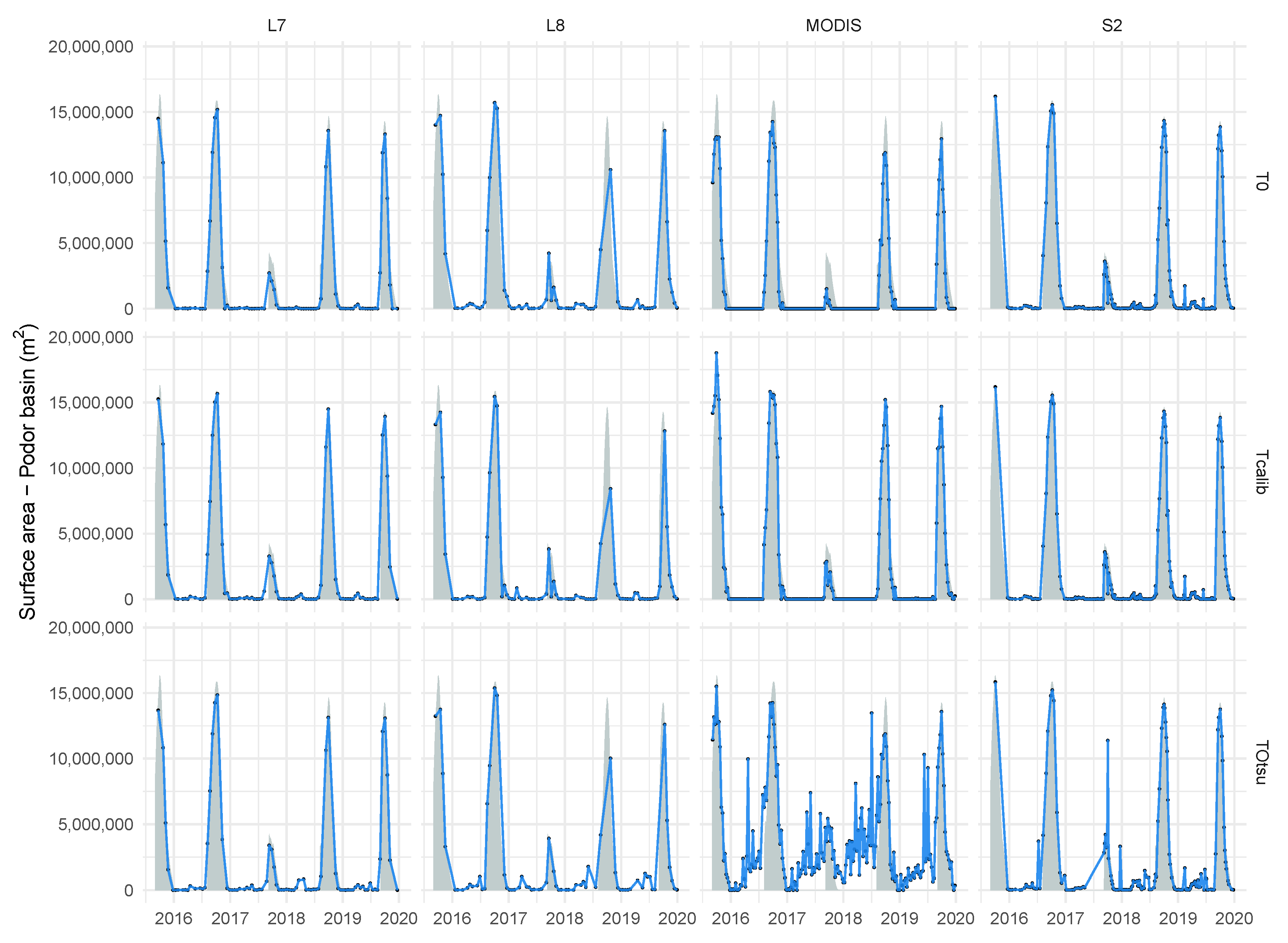
The rising availability of remote sensing imagery provides increased opportunities for surface water monitoring. Multi-sensor is the future direction [42], and this research provides essential information into the relative benefits of combining sensors over different periods of the past twenty years (1999–2019). Numerous multi-sensor approaches have been developed to combine the observations from a virtual constellation of satellites and provide greater temporal resolution, notably in cloud affected settings and periods. Whitcraft et al. [19], Claverie et al. [36] notably argued for the need to combine the Landsat 7, Landsat 8, as well as Sentinel-2A and 2B satellites, to take full advantage of the rising spatial resolution (up to 10 m on certain S2 bands). However, our research shows that for earlier years, coarse resolution, high repetitivity MODIS imagery remains essential even in the monitoring of small (19 km 2 ) water bodies and should not be overlooked in favour of higher resolution sensors.
Previous research notably showed that MODIS was suited to the study of hydrological systems superior to 10,000 km 2 [8]. Khandelwal et al. [17] using a supervised classification algorithm based on Support Vector Machines (SVMs) showed that MODIS imagery could be used to study water trends on large lakes ranging between 240 km 2 and 5380 km 2 . Our results show that site-specific thresholds on MNDWI can be used to monitor daily long-term variations of flood dynamics under 19 km 2 and reduce the RMSE by 50% compared to Otsu segmentation. Field calibrated thresholds are shown to be most suited with MODIS to force a lower threshold and take into account the presence of shallow waters and flooded vegetation in the pixels, supporting results on other wetlands [12].
Global Surface Water datasets [23] are often referred to as the best attempt to provide water maps at high resolution [42] and many global datasets are developed solely on Landsat and Sentinel archives [22,23,26,36]. The results demonstrate the clear limitations before 2013 of GSW datasets built on one image every 30 days, to monitor flood dynamics in floodplains. These are notably insufficient to reproduce surface water dynamics in the smallest (<1 km 2 ), temporary water bodies with flash floods [7,82,83] and are also insufficient in floodplains with slow flood dynamics. Using the full Landsat archive provides observations every 24 days on average over 1999–2019, but the benefits of integrating additional data sources remain indisputable, e.g., to capture flood peaks in 2003 and 2004 missed here by Landsat. Despite cloud presence during the flood rise, optical imagery is shown here to be sufficient to monitor surface water variations. Combining or fusing optical imagery with active radar imagery such as Sentinel-1 may be relevant in areas or periods where cloud presence is more frequent and problematic [84], notably during the monsoon season at tropical latitudes. To capture the benefits of both Landsat spatial resolution and MODIS temporal resolution, the integration of data fusion methods such as the ESTARFM algorithm [85,86] within GEE has the potential to raise performance further. Similarly, when focussing on smaller hydrological objects or on low water periods, pansharpening and subpixel approaches [42] may provide benefits and should be supported by the integration of the adequate panchromatic bands and algorithms in the GEE platform.
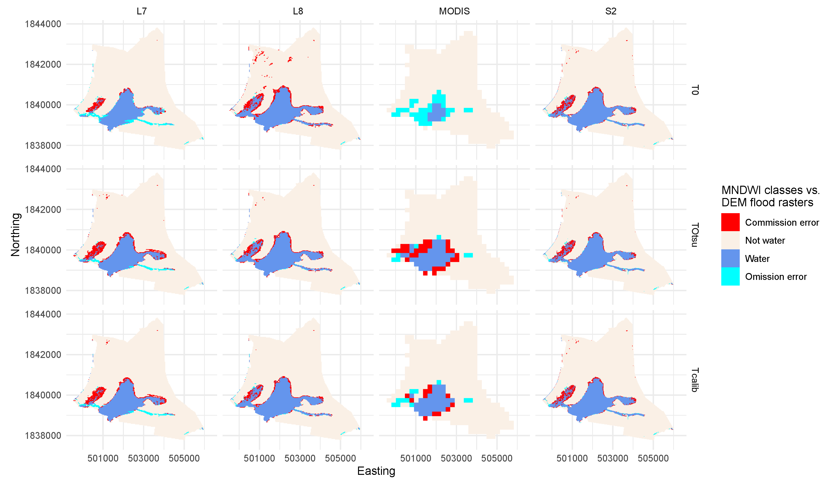
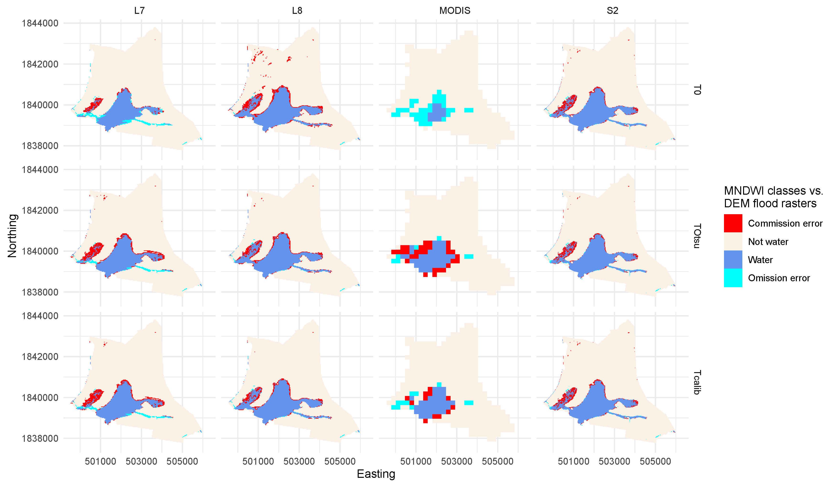
The full MODIS and Landsat surface reflectance imagery have been integrated in Google Earth Engines, and access to these cloud geoprocessing capacities here greatly reduces the download and treatment times. Level 2 surface reflectance Sentinel-2 imagery for our region of interest is however only available since 16 December 2018, and integration within GEE of the full Level 2 products will be a welcome addition for the academic community. Results based on Level 1C imagery nevertheless show here good stability and consistency between sensors, supporting similar studies using digital numbers and top of atmosphere reflectance [27,64,87]. Undetected clouds notably cause problems with the Otsu algorithm on Sentinel-2 imagery here. These are less prevalent with Landsat imagery, which benefits from clouds masks produced by the improved CFmask algorithm. Considering the relative weaknesses of default cloud algorithms for MODIS and Sentinel-2 compared to CFmask, integration within GEE of improved cloud masks or efficient cloud algorithms should be investigated to assess the potential improvements. Baetens et al. [88] showed that the Fmask or MAJA algorithms could improve further on the Sen2Cor approach employed by ESA. Nevertheless, optically thin clouds will remain challenging to identify and may be omitted by CFMask, including on Landsat imagery.
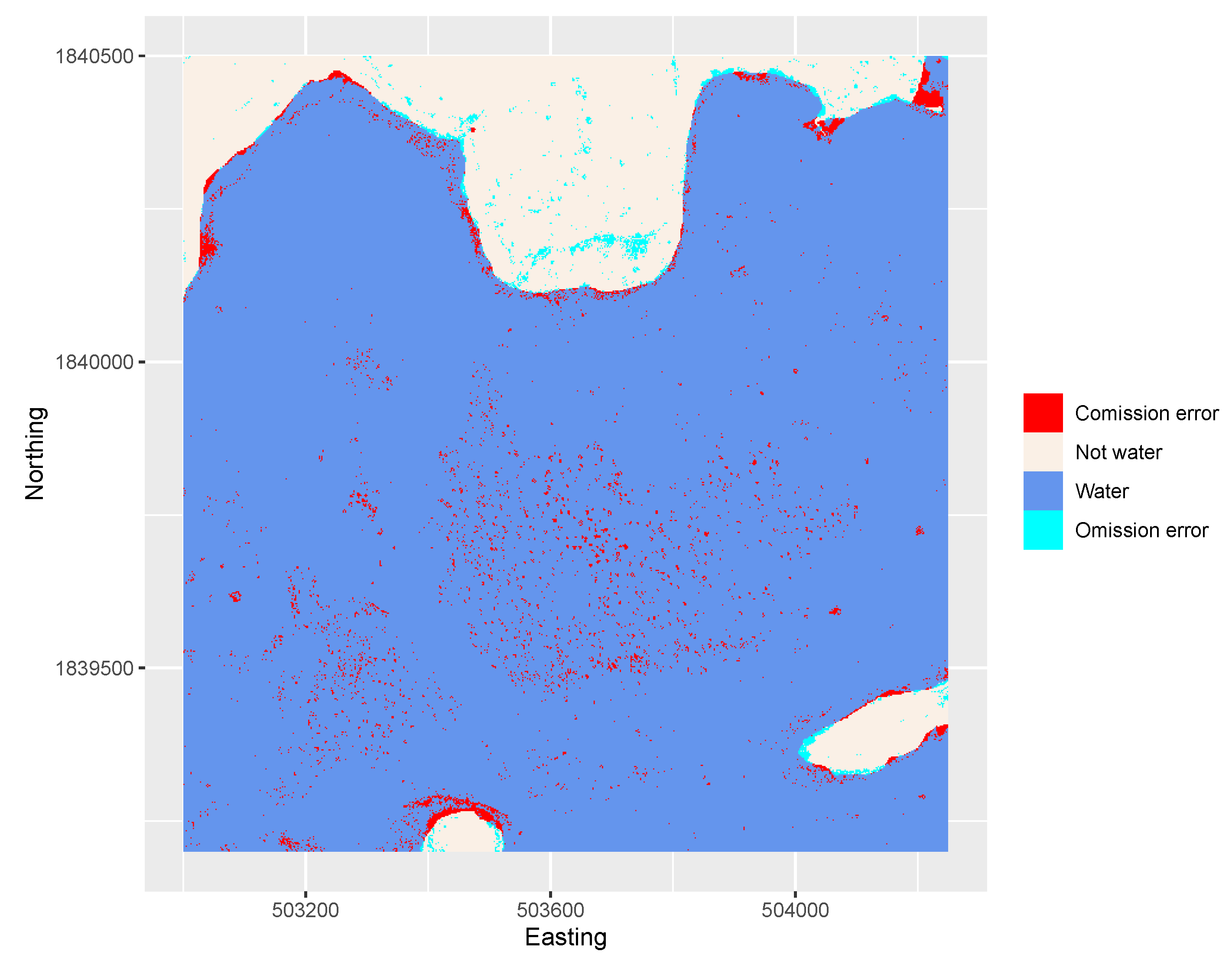
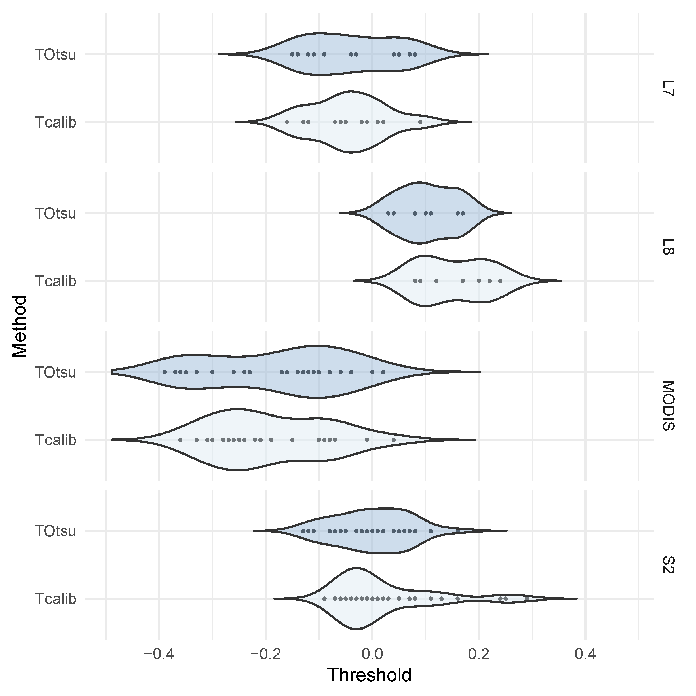
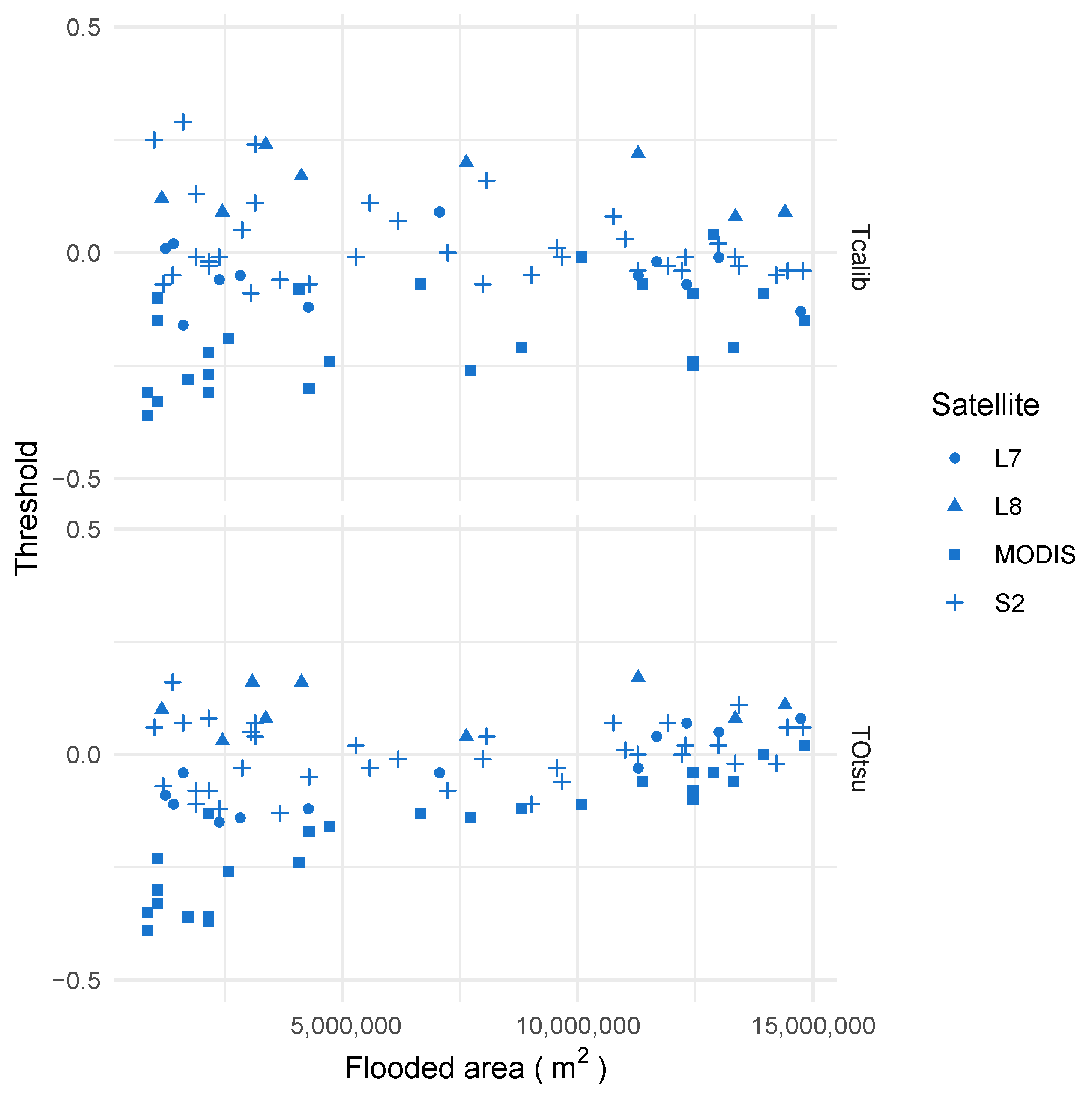
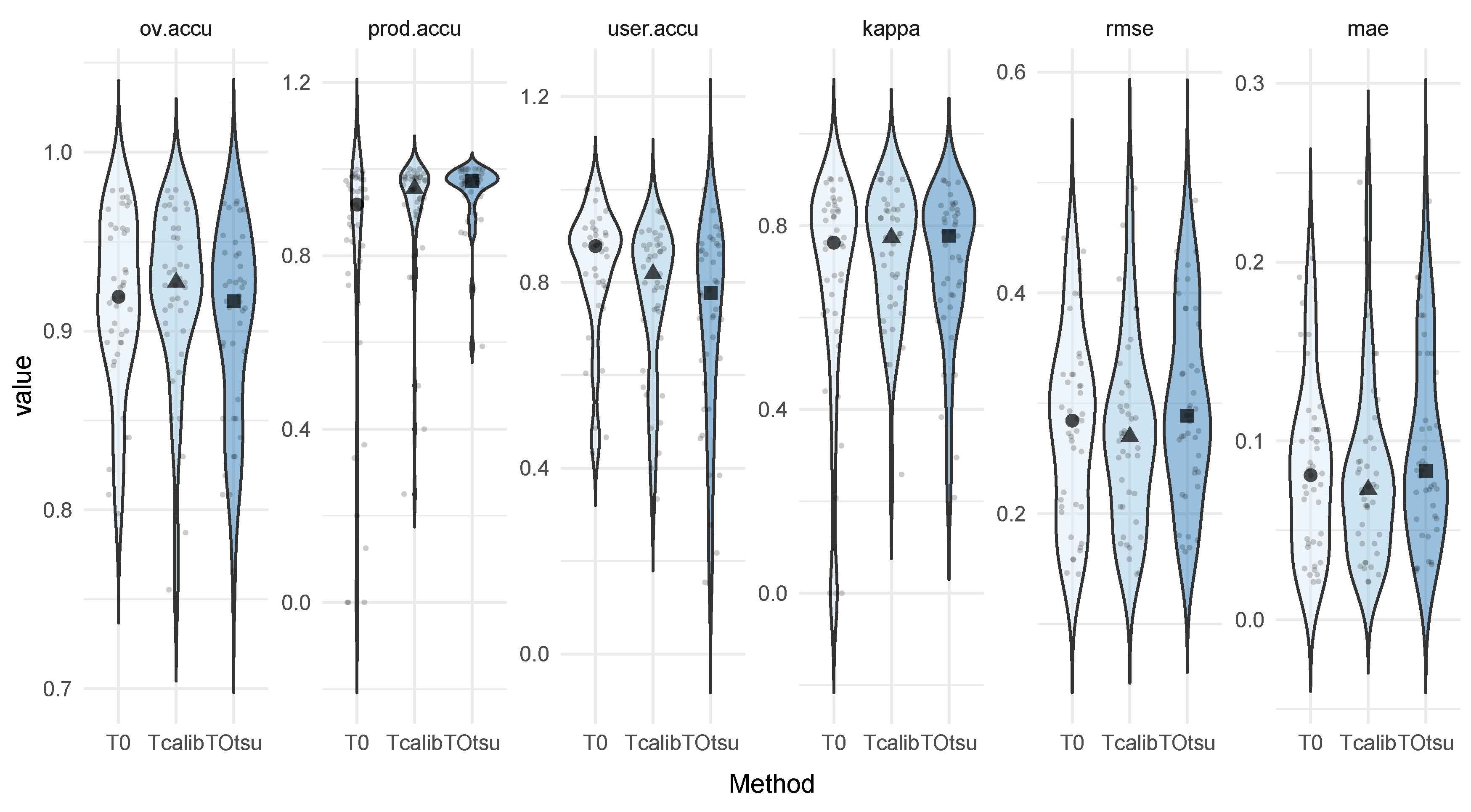
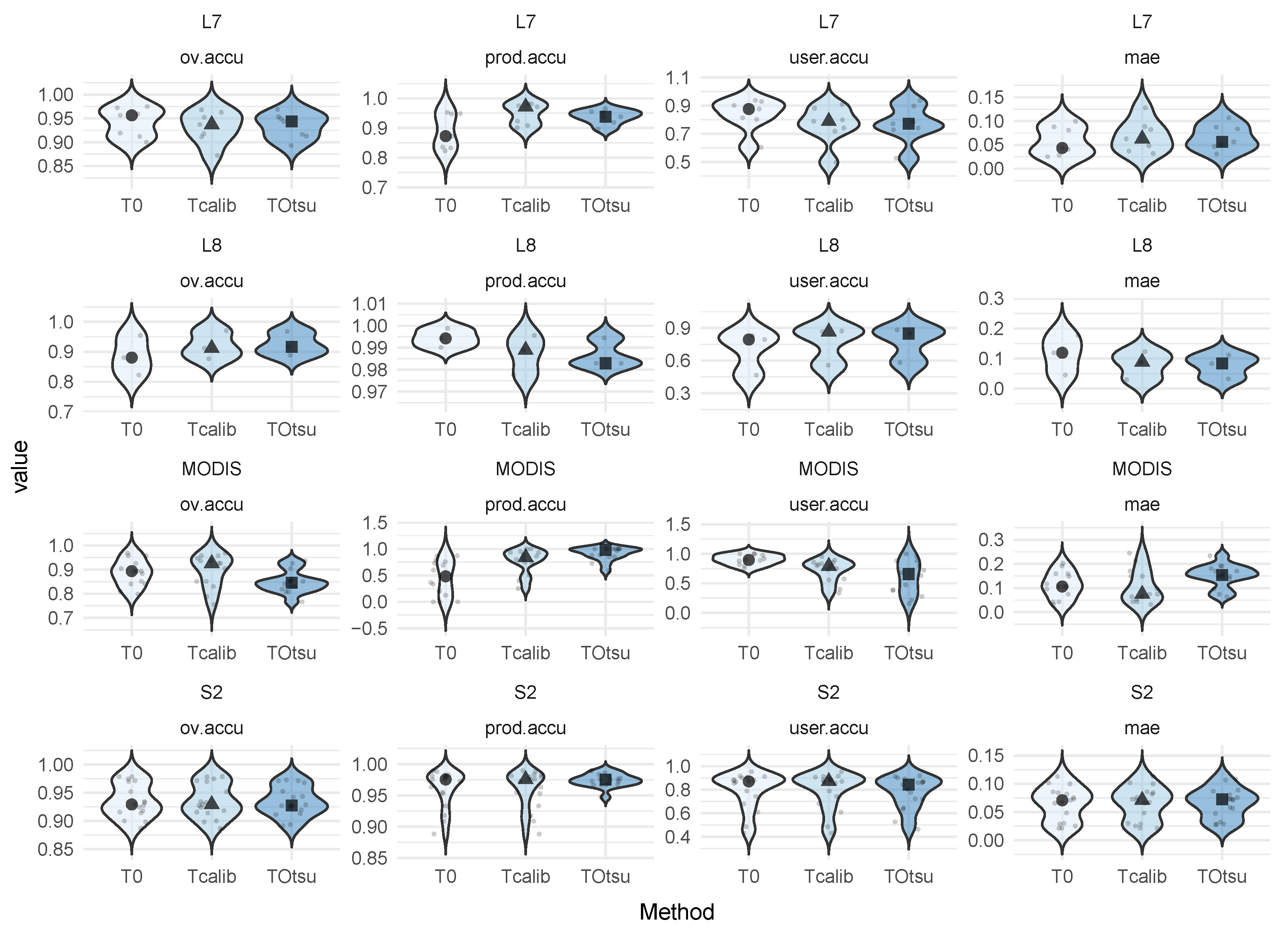
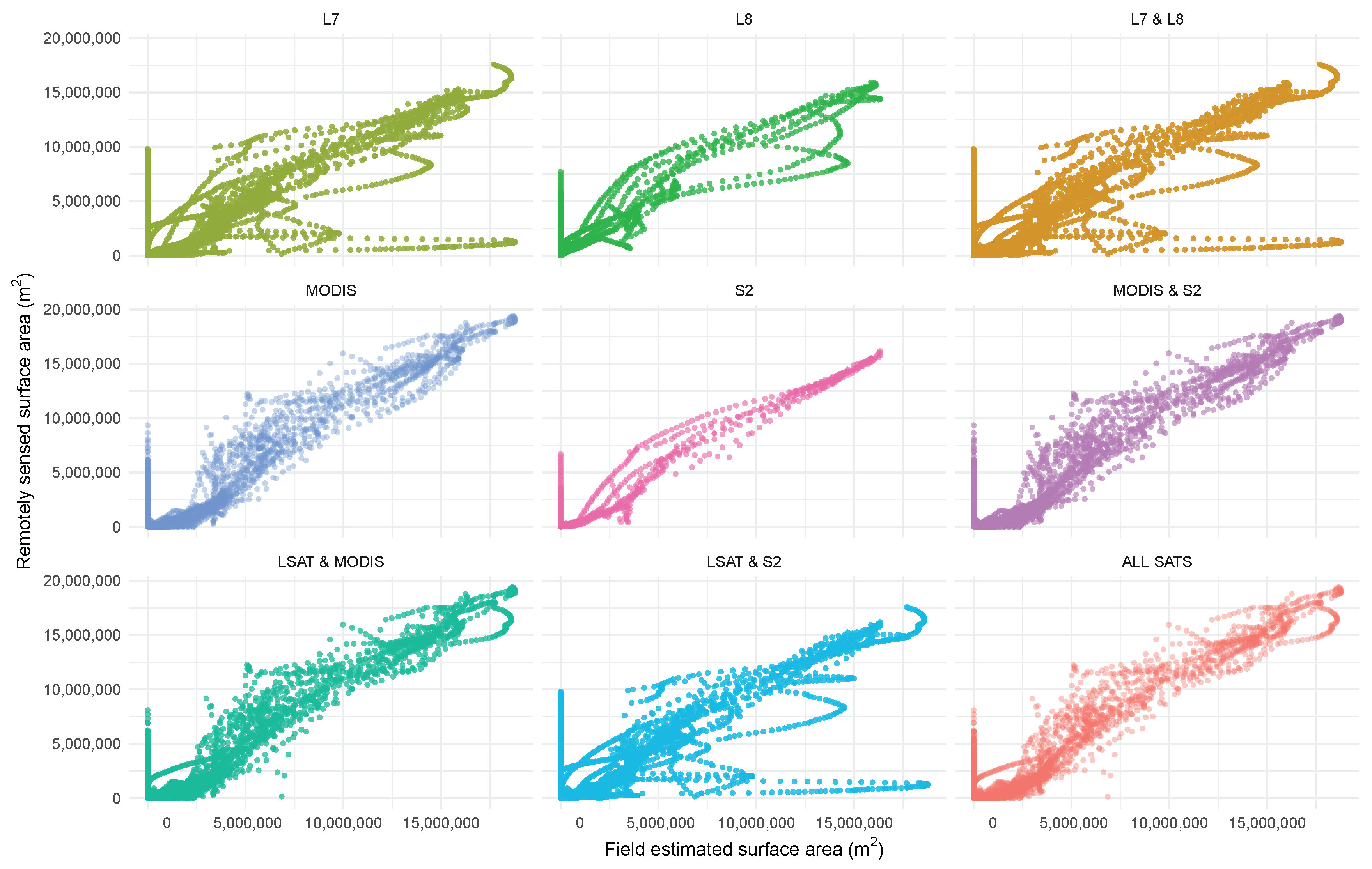
Water classification using MNDWI reach very high levels of accuracy with the sensor-specific optimal thresholding methods developed in this paper. The results show here that no single method is suitable for all sensors due to the specificities of each sensor and the particularities of long-term monitoring. Otsu segmentation, known to perform well [64], notably suffers due to the temporary nature of water bodies and the sharp decline in water areas. Even though image growing was used to specifically include the permanent river areas, a decline in the performance of the Otsu algorithm was observed as water occupies too small a fraction, around 10% according to Lee et al. [89]. Water indices and especially MNDWI are well suited to multi-temporal water mapping [42]; however, alternate classification approaches may help improve performance, especially in different settings. Substituting green bands for ultra-blue and blue bands in these water indices may provide benefits in open water environments with low turbidity, while red band-based water indices may assist classification in water bodies with high suspended sediment loads [64]. Machine learning algorithms such as random forest integrated into GEE, and used here on the UAV data, are known to perform well on complex imagery, though their use can be more resource intensive, requiring additional training data and making them less suited to long-term studies [42]. Amani et al. [39] with a large amount of field samples used a random forest approach to map Canadian wetlands, but overall accuracy reached 71% with over 34% and 37% of omission and commission errors, respectively. These errors can be explained by the difficulties in heterogeneous wetland environments, where water bodies are not continuous objects due to the presence of flooded vegetation and shallow disconnected meanders. The GSW datasets based on machine learning systems have also been shown to perform less well in mixed water environments found in small water bodies and wetlands [7,83].
In parallel, these results highlight the value of long-term hydrological observations to assess the accuracy and skill of remote sensing datasets. Remote sensing studies often rely on alternate high resolution satellite imagery or, where possible, in situ observations [90], such as geolocalised sampling using GPS points, transects and contours to train and evaluate classifications. Validation is often based on random sampling of water bodies, but is restricted, for reasons of cost or feasibility, in the number of observations over time and rarely informs about the suitability to reproduce daily water dynamics in long-term monitoring [7,42,91]. Many global water datasets are similarly developed against ground truth data for open water bodies, which as discussed above, can reduce their value in wetlands and other heterogeneous water environments. Long-term hydrological observatories, supported by citizen science observations [92], must then be encouraged to support the development and assessment of remote sensing products and algorithms relevant to the water community. New products such as higher accuracy DEMs from Tandem-X [3] or localised UAV-based methods [93] also have the potential to provide valuable ground truth data. Finally, our results point to the importance of using multiple metrics in classification accuracy assessments. Overall accuracy can lead to difficult or incomplete interpretation [77] of classifications, due to the effects of class prevalence [78], i.e., correctly classified non-water pixels as water recedes for instance, and minor (two to three percentage points) differences in accuracy can cause large differences on the resulting surface areas.

5. Conclusions

Detailed comparison of four major sources of optical Earth observations against extensive ground truth data highlight the heterogeneous performance of three MNDWI thresholding methods. The Otsu algorithm (TOtsu) is shown to be highly effective to classify selected images from Sentinel-2 and Landsat 8 sensors. However, when used in conditions of long-term observations in temporary water bodies, the Otsu method underperforms compared to a default threshold (T0). On Landsat 7, a default threshold performs best, while for MODIS imagery, a site-specific data intensive approach is essential to reduce the underestimation of pixels where water and flooded vegetation gather. The sensor-specific MNDWI thresholding methods identified here result in significant improvements in the accuracy of the mapped flooded areas. MODIS, despite its 500 m spatial resolution, performs remarkably well with a calibrated threshold and demonstrates its value in monitoring hydrological systems as small as 19 km 2 . Landsat 7, even after 2003 and gap filling for the scan line failure, provides remarkably good observations, comparable with Sentinel-2 in terms of RMSE.
In long-term water mapping, Landsat imagery before 2013 fails to capture substantial information, in terms of flood peaks and flood dynamics. Combining multiple sensors’ observations is essential, and before 2013, it is recommended to integrate MODIS and Landsat observations notably on water bodies of several hundred hectares with similar temporary flood dynamics. After 2013, the combination of Landsat 7 and Landsat 8 becomes sufficient, and integrating MODIS observations can degrade performance marginally. The constellation of Sentinel-2A and 2B satellites offering high spatial and temporal resolution performs well in surface water monitoring, and integrating MODIS observations degrades overall accuracy. The integration of Landsat and Sentinel-2 yields modest improvements. This has important implications when developing long-term consolidated datasets designed to be used by researchers and stakeholders to understand flood variations, water balance modelling and water availability of wetlands and floodplains.
The frequent surface water maps produced by this semi-automated multi-sensor approach may be used to understand how water overflows into the floodplain and improve hydrological representations of hysteresis as water recedes. Supported by Google Earth Engines’ geoprocessing capacities, this approach can be applied across entire wetlands and floodplains to provide high resolution maps of flooded areas, calibrate hydrological models, improve local digital elevation models and investigate relationships with agricultural practices.

Author Contributions

Conceptualization, A.O.; methodology, A.O., J.-C.P., and J.-C.B.; formal analysis, A.O., D.M., J.-C.P., and J.-C.B.; writing, original draft preparation, A.O., J.-C.P., and J.-C.B.; writing, review and editing, A.O., J.-C.P., J.-C.B., F.B., A.B., H.D., D.D., L.D., and S.S.; supervision, A.O.; project administration, A.O., D.D., A.B., L.D., S.S., and J.-C.P.; funding acquisition, A.O., D.D., A.B., L.D., S.S., and J.-C.P. All authors read and agreed to the published version of the manuscript.

Funding

This research was partly funded by the ANR LEAP-AGRI WAGRINNOVA (grant number ANR-18-LEAP-0002) and EU-funded AICS N.03/2020/WEFE-SENEGAL projects.

Acknowledgments

The authors are grateful for the hydrological data supplied by the OMVS, as well as the Landsat and MODIS data made available by USGS and the Sentinel-2 data made available by ESA in Google Earth Engines. We also thank three anonymous reviewers and the Academic Editors for their valuable comments.

Conflicts of Interest

The authors declare no conflict of interest.

Appendix A

Figure A1. Available observations in Google Earth Engines for the region of interest from the Landsat, MODIS and Sentinel-2 satellites over the 1999–2019 period.
Remotesensing 12 03157 g0a1
Table A1. Elevations of the 22 samples points measured using RTK GPS to assess and correct DTM altitudes.
Sample PointRTK GPS Altitude (m)DTM Altitude (m)Difference (cm)
P14.3213.91440.7
P23.7733.57020.3
P33.6263.28234.4
P43.3033.00429.9
P53.1863.04813.8
PPC2.6262.26835.8
T13.9163.58033.6
T23.6113.33028.1
T33.7013.37432.7
T43.7723.45931.3
T53.4623.16230.0
T63.8673.59327.4
T73.0972.77532.2
T83.6233.31830.5
T92.9662.61335.3
T103.0472.82322.4
T112.6652.27139.4
T124.2913.96532.6
T134.3723.97539.7
T143.7613.43732.4
T153.5343.14738.7
T163.6663.33033.6
Average31.58
Standard deviation6.31

References

  1. Montanari, A.; Young, G.; Savenije, H.H.G.; Hughes, D.; Wagener, T.; Ren, L.L.; Koutsoyiannis, D.; Cudennec, C.; Toth, E.; Grimaldi, S.; et al. Panta Rhei—Everything Flows: Change in hydrology and society—The IAHS Scientific Decade 2013–2022. Hydrol. Sci. J. 2013, 58, 1256–1275. [Google Scholar] [CrossRef]
  2. Bates, P.D.; Neal, J.C.; Alsdorf, D.; Schumann, G.J.P. Observing Global Surface Water Flood Dynamics. Surv. Geophys. 2014, 35, 839–852. [Google Scholar] [CrossRef]
  3. Hawker, L.; Neal, J.; Bates, P. Accuracy assessment of the TanDEM-X 90 Digital Elevation Model for selected floodplain sites. Remote Sens. Environ. 2019, 232, 111319. [Google Scholar] [CrossRef]
  4. Liebe, J.; van de Giesen, N.; Andreini, M. Estimation of small reservoir storage capacities in a semi-arid environment. Phys. Chem. Earth Parts A/B/C 2005, 30, 448–454. [Google Scholar] [CrossRef]
  5. Soti, V.; Tran, A.; Bailly, J.S.; Puech, C.; Seen, D.L.; Bégué, A. Assessing optical earth observation systems for mapping and monitoring temporary ponds in arid areas. Int. J. Appl. Earth Obs. Geoinf. 2009, 11, 344–351. [Google Scholar] [CrossRef] [Green Version]
  6. Gardelle, J.; Hiernaux, P.; Kergoat, L.; Grippa, M. Less rain, more water in ponds: A remote sensing study of the dynamics of surface waters from 1950 to present in pastoral Sahel (Gourma region, Mali). Hydrol. Earth Syst. Sci. 2010, 14, 309–324. [Google Scholar] [CrossRef] [Green Version]
  7. Ogilvie, A.; Belaud, G.; Massuel, S.; Mulligan, M.; Goulven, P.L.; Calvez, R. Surface water monitoring in small water bodies: Potential and limits of multi-sensor Landsat time series. Hydrol. Earth Syst. Sci. 2018, 22, 4349. [Google Scholar] [CrossRef] [Green Version]
  8. Sakamoto, T.; Van Nguyen, N.; Kotera, A.; Ohno, H.; Ishitsuka, N.; Yokozawa, M. Detecting temporal changes in the extent of annual flooding within the Cambodia and the Vietnamese Mekong Delta from MODIS time-series imagery. Remote Sens. Environ. 2007, 109, 295–313. [Google Scholar] [CrossRef]
  9. Huang, C.; Chen, Y.; Wu, J. Mapping spatio-temporal flood inundation dynamics at large river basin scale using time-series flow data and MODIS imagery. Int. J. Appl. Earth Obs. Geoinf. 2014, 26, 350–362. [Google Scholar] [CrossRef]
  10. Bergé-Nguyen, M.; Crétaux, J.F. Inundations in the Inner Niger Delta: Monitoring and Analysis Using MODIS and Global Precipitation Datasets. Remote Sens. 2015, 7, 2127–2151. [Google Scholar] [CrossRef] [Green Version]
  11. Kuenzer, C.; Dech, S.; Wagner, W. (Eds.) Remote Sensing and Digital Image Processing; Remote Sensing Time Series; Springer International Publishing: Cham, Switzerland, 2015; Volume 22. [Google Scholar] [CrossRef]
  12. Ogilvie, A.; Belaud, G.; Delenne, C.; Bailly, J.S.; Bader, J.C.; Oleksiak, A.; Ferry, L.; Martin, D. Decadal monitoring of the Niger Inner Delta flood dynamics using MODIS optical data. J. Hydrol. 2015, 523, 368–383. [Google Scholar] [CrossRef] [Green Version]
  13. Guo, M.; Li, J.; Sheng, C.; Xu, J.; Wu, L. A Review of Wetland Remote Sensing. Sensors 2017, 17, 777. [Google Scholar] [CrossRef] [PubMed] [Green Version]
  14. Aires, F.; Venot, J.P.; Massuel, S.; Gratiot, N.; Pham-Duc, B.; Prigent, C. Surface water evolution (2001–2017) at the Cambodia/Vietnam border in the upper mekong delta using satellite MODIS observations. Remote Sens. 2020, 12, 800. [Google Scholar] [CrossRef] [Green Version]
  15. Carroll, M.; Townshend, J.; DiMiceli, C.; Noojipady, P.; Sohlberg, R. A new global raster water mask at 250 m resolution. Int. J. Digit. Earth 2009, 2, 291–308. [Google Scholar] [CrossRef]
  16. Klein, I.; Gessner, U.; Dietz, A.J.; Kuenzer, C. Global WaterPack—A 250 m resolution dataset revealing the daily dynamics of global inland water bodies. Remote Sens. Environ. 2017, 198, 345–362. [Google Scholar] [CrossRef]
  17. Khandelwal, A.; Karpatne, A.; Marlier, M.E.; Kim, J.; Lettenmaier, D.P.; Kumar, V. An approach for global monitoring of surface water extent variations in reservoirs using MODIS data. Remote Sens. Environ. 2017, 202, 113–128. [Google Scholar] [CrossRef]
  18. D’Andrimont, R.; Defourny, P. Monitoring African water bodies from twice-daily MODIS observation. GISci. Remote Sens. 2018, 55, 130–153. [Google Scholar] [CrossRef]
  19. Whitcraft, A.; Becker-Reshef, I.; Killough, B.; Justice, C. Meeting Earth Observation Requirements for Global Agricultural Monitoring: An Evaluation of the Revisit Capabilities of Current and Planned Moderate Resolution Optical Earth Observing Missions. Remote Sens. 2015, 7, 1482–1503. [Google Scholar] [CrossRef] [Green Version]
  20. Feng, M.; Sexton, J.O.; Channan, S.; Townshend, J.R. A global, high-resolution (30-m) inland water body dataset for 2000: First results of a topographic-spectral classification algorithm. Int. J. Digit. Earth 2016, 9, 113–133. [Google Scholar] [CrossRef] [Green Version]
  21. Verpoorter, C.; Kutser, T.; Seekell, D.A.; Tranvik, L.J. A Global Inventory of Lakes Based on High-Resolution Satellite Imagery. Geophys. Res. Lett. 2014, 41, 6396–6402. [Google Scholar] [CrossRef]
  22. Yamazaki, D.; Trigg, M.A.; Ikeshima, D. Development of a global ∼90 m water body map using multi-temporal Landsat images. Remote Sens. Environ. 2015, 171, 337–351. [Google Scholar] [CrossRef]
  23. Pekel, J.F.; Cottam, A.; Gorelick, N.; Belward, A.S. High-resolution mapping of global surface water and its long-term changes. Nature 2016, 540, 418–422. [Google Scholar] [CrossRef] [PubMed]
  24. Gorelick, N.; Hancher, M.; Dixon, M.; Ilyushchenko, S.; Thau, D.; Moore, R. Google Earth Engine: Planetary-scale geospatial analysis for everyone. Remote Sens. Environ. 2017, 202, 18–27. [Google Scholar] [CrossRef]
  25. Busker, T.; De Roo, A.; Gelati, E.; Schwatke, C.; Adamovic, M.; Bisselink, B.; Pekel, J.F.; Cottam, A. A global lake and reservoir volume analysis using a surface water dataset and satellite altimetry. Hydrol. Earth Syst. Sci. 2019, 23, 669–690. [Google Scholar] [CrossRef] [Green Version]
  26. Donchyts, G.; Baart, F.; Winsemius, H.; Gorelick, N.; Kwadijk, J.; van de Giesen, N. Earth’s surface water change over the past 30 years. Nat. Clim. Chang. 2016, 6, 810–813. [Google Scholar] [CrossRef]
  27. Yang, X.; Qin, Q.; Yésou, H.; Ledauphin, T.; Koehl, M.; Grussenmeyer, P.; Zhu, Z. Monthly estimation of the surface water extent in France at a 10-m resolution using Sentinel-2 data. Remote Sens. Environ. 2020, 244. [Google Scholar] [CrossRef]
  28. Aires, F.; Prigent, C.; Fluet-Chouinard, E.; Yamazaki, D.; Papa, F.; Lehner, B. Comparison of visible and multi-satellite global inundation datasets at high-spatial resolution. Remote Sens. Environ. 2018, 216. [Google Scholar] [CrossRef] [Green Version]
  29. Yao, F.; Wang, J.; Wang, C.; Crétaux, J.F. Constructing long-term high-frequency time series of global lake and reservoir areas using Landsat imagery. Remote Sens. Environ. 2019, 232, 111210. [Google Scholar] [CrossRef]
  30. Prigent, C.; Papa, F.; Aires, F.; Rossow, W.B.; Matthews, E. Global inundation dynamics inferred from multiple satellite observations, 1993–2000. J. Geophys. Res. 2007, 112, D12107. [Google Scholar] [CrossRef]
  31. Papa, F.; Prigent, C.; Aires, F.; Jimenez, C.; Rossow, W.B.; Matthews, E. Interannual variability of surface water extent at the global scale, 1993–2004. J. Geophys. Res. 2010, 115, D12111. [Google Scholar] [CrossRef]
  32. Aires, F.; Miolane, L.; Prigent, C.; Pham, B.; Fluet-Chouinard, E.; Lehner, B.; Papa, F. A global dynamic long-term inundation extent dataset at high spatial resolution derived through downscaling of satellite observations. J. Hydrometeorol. 2017, 18, 1305–1325. [Google Scholar] [CrossRef]
  33. Musa, Z.N.; Popescu, I.; Mynett, A. A review of applications of satellite SAR, optical, altimetry and DEM data for surface water modelling, mapping and parameter estimation. Hydrol. Earth Syst. Sci. 2015, 19, 3755–3769. [Google Scholar] [CrossRef] [Green Version]
  34. Padró, J.C.; Pons, X.; Aragonés, D.; Díaz-Delgado, R.; García, D.; Bustamante, J.; Pesquer, L.; Domingo-Marimon, C.; González-Guerrero, Ò.; Cristóbal, J.; et al. Radiometric Correction of Simultaneously Acquired Landsat-7/Landsat-8 and Sentinel-2A Imagery Using Pseudoinvariant Areas (PIA): Contributing to the Landsat Time Series Legacy. Remote Sens. 2017, 9, 1319. [Google Scholar] [CrossRef] [Green Version]
  35. Carrasco, L.; O’Neil, A.; Morton, R.; Rowland, C. Evaluating Combinations of Temporally Aggregated Sentinel-1, Sentinel-2 and Landsat 8 for Land Cover Mapping with Google Earth Engine. Remote Sens. 2019, 11, 288. [Google Scholar] [CrossRef] [Green Version]
  36. Claverie, M.; Ju, J.; Masek, J.G.; Dungan, J.L.; Vermote, E.F.; Roger, J.C.; Skakun, S.V.; Justice, C. The Harmonized Landsat and Sentinel-2 surface reflectance data set. Remote Sens. Environ. 2018, 219, 145–161. [Google Scholar] [CrossRef]
  37. Yamazaki, D.; Trigg, M.A. Hydrology: The dynamics of Earth’s surface water. Nature 2016, 540, 348–349. [Google Scholar] [CrossRef] [Green Version]
  38. Mueller, N.; Lewis, A.; Roberts, D.; Ring, S.; Melrose, R.; Sixsmith, J.; Lymburner, L.; McIntyre, A.; Tan, P.; Curnow, S.; et al. Water observations from space: Mapping surface water from 25years of Landsat imagery across Australia. Remote Sens. Environ. 2016, 174, 341–352. [Google Scholar] [CrossRef] [Green Version]
  39. Amani, M.; Brisco, B.; Afshar, M.; Mirmazloumi, S.M.; Mahdavi, S.; Mirzadeh, S.M.J.; Huang, W.; Granger, J. A generalized supervised classification scheme to produce provincial wetland inventory maps: An application of Google Earth Engine for big geo data processing. Big Earth Data 2019, 3, 378–394. [Google Scholar] [CrossRef]
  40. Mahdavi, S.; Salehi, B.; Granger, J.; Amani, M.; Brisco, B.; Huang, W. Remote sensing for wetland classification: A comprehensive review. GISci. Remote Sens. 2018, 55, 623–658. [Google Scholar] [CrossRef]
  41. Mahdianpari, M.; Salehi, B.; Mohammadimanesh, F.; Homayouni, S.; Gill, E. The First Wetland Inventory Map of Newfoundland at a Spatial Resolution of 10 m Using Sentinel-1 and Sentinel-2 Data on the Google Earth Engine Cloud Computing Platform. Remote Sens. 2018, 11, 43. [Google Scholar] [CrossRef] [Green Version]
  42. Huang, C.; Chen, Y.; Zhang, S.; Wu, J. Detecting, Extracting, and Monitoring Surface Water From Space Using Optical Sensors: A Review. Rev. Geophys. 2018, 56, 333–360. [Google Scholar] [CrossRef]
  43. Sun, Z.; Xu, R.; Du, W.; Wang, L.; Lu, D. High-Resolution Urban Land Mapping in China from Sentinel 1A/2 Imagery Based on Google Earth Engine. Remote Sens. 2019, 11, 752. [Google Scholar] [CrossRef] [Green Version]
  44. Markert, K.N.; Chishtie, F.; Anderson, E.R.; Saah, D.; Griffin, R.E. On the merging of optical and SAR satellite imagery for surface water mapping applications. Results Phys. 2018, 9, 275–277. [Google Scholar] [CrossRef]
  45. Pahlevan, N.; Chittimalli, S.K.; Balasubramanian, S.V.; Vellucci, V. Sentinel-2/Landsat-8 product consistency and implications for monitoring aquatic systems. Remote Sens. Environ. 2019, 220. [Google Scholar] [CrossRef]
  46. Nguyen, M.D.; Baez-Villanueva, O.M.; Bui, D.D.; Nguyen, P.T.; Ribbe, L. Harmonization of Landsat and Sentinel 2 for Crop Monitoring in Drought Prone Areas: Case Studies of Ninh Thuan (Vietnam) and Bekaa (Lebanon). Remote Sens. 2020, 12, 281. [Google Scholar] [CrossRef] [Green Version]
  47. Bader, J.C.; Belaud, G.; Lamagat, J.P.; Ferret, T.; Vauchel, P. Modélisation de propagation d’écoulement entre lits mineur et majeur sur les fleuves Sénégal et Niger. Hydrol. Sci. J. 2017, 62, 447–466. [Google Scholar] [CrossRef]
  48. Poussin, J.C.; Martin, D.; Bader, J.C.; Dia, D.; Seck, S.M.; Ogilvie, A. Variabilité agro-hydrologique des cultures de décrue. Une étude de cas dans la moyenne vallée du fleuve Sénégal. Cah. Agric. 2020, 29, 23. [Google Scholar] [CrossRef]
  49. Hagolle, O.; Huc, M.; Pascual, D.; Dedieu, G. A Multi-Temporal and Multi-Spectral Method to Estimate Aerosol Optical Thickness over Land, for the Atmospheric Correction of FormoSat-2, LandSat, VENS and Sentinel-2 Images. Remote Sens. 2015, 7, 2668–2691. [Google Scholar] [CrossRef] [Green Version]
  50. Louis, J.; Debaecker, V.; Pflug, B.; Main-Knorn, M.; Bieniarz, J.; Mueller-Wilm, U.; Cadau, E.; Gascon, F. Sentinel-2 SEN2COR: L2A Processor for Users. In Proceedings of the ESA Living Planet Symposium 2016, Prague, Czech Republic, 9–13 May 2016; pp. 1–8. [Google Scholar]
  51. Zhu, Z.; Woodcock, C.E. Object-based cloud and cloud shadow detection in Landsat imagery. Remote Sens. Environ. 2012, 118, 83–94. [Google Scholar] [CrossRef]
  52. Foga, S.; Scaramuzza, P.L.; Guo, S.; Zhu, Z.; Dilley, R.D.; Beckmann, T.; Schmidt, G.L.; Dwyer, J.L.; Joseph Hughes, M.; Laue, B. Cloud detection algorithm comparison and validation for operational Landsat data products. Remote Sens. Environ. 2017, 194, 379–390. [Google Scholar] [CrossRef] [Green Version]
  53. USGS. Landsat 4-7 Surface Reflectance (LEDAPS) Product Guide—Version 2.0; Technical Report; EROS: Sioux Falls, SD, USA, 2019.
  54. USGS. Land Surface Reflectance Code LaSRC Product Guide—Version 2.0; Technical Report; EROS: Sioux Falls, SD, USA, 2019.
  55. Roger, J.; Vermote, E.; Ray, J. MODIS Surface Reflectance User’s Guide. Collection 6.; Technical Report; MODIS Land Surface Reflectance Science Computing Facility: Greenbelt, MD, USA, 2015. [Google Scholar]
  56. Coluzzi, R.; Imbrenda, V.; Lanfredi, M.; Simoniello, T. A first assessment of the Sentinel-2 Level 1-C cloud mask product to support informed surface analyses. Remote Sens. Environ. 2018, 217, 426–443. [Google Scholar] [CrossRef]
  57. Zhang, F.; Li, J.; Zhang, B.; Shen, Q.; Ye, H.; Wang, S.; Lu, Z. A simple automated dynamic threshold extraction method for the classification of large water bodies from landsat-8 OLI water index images. Int. J. Remote Sens. 2018, 39, 3429–3451. [Google Scholar] [CrossRef]
  58. Xu, H. Modification of normalised difference water index (NDWI) to enhance open water features in remotely sensed imagery. Int. J. Remote Sens. 2006, 27, 3025–3033. [Google Scholar] [CrossRef]
  59. Ji, L.; Zhang, L.; Wylie, B. Analysis of Dynamic Thresholds for the Normalized Difference Water Index. Photogramm. Eng. Remote Sens. 2009, 75, 1307–1317. [Google Scholar] [CrossRef]
  60. Li, W.; Du, Z.; Ling, F.; Zhou, D.; Wang, H.; Gui, Y.; Sun, B.; Zhang, X. A Comparison of Land Surface Water Mapping Using the Normalized Difference Water Index from TM, ETM+ and ALI. Remote Sens. 2013, 5, 5530–5549. [Google Scholar] [CrossRef] [Green Version]
  61. McFeeters, S.K. The use of the Normalized Difference Water Index (NDWI) in the delineation of open water features. Int. J. Remote Sens. 1996, 17, 1425–1432. [Google Scholar] [CrossRef]
  62. Feyisa, G.L.; Meilby, H.; Fensholt, R.; Proud, S.R. Automated Water Extraction Index: A new technique for surface water mapping using Landsat imagery. Remote Sens. Environ. 2014, 140, 23–35. [Google Scholar] [CrossRef]
  63. Guo, Q.; Pu, R.; Li, J.; Cheng, J. A weighted normalized difference water index for water extraction using landsat imagery. Int. J. Remote Sens. 2017, 38, 5430–5445. [Google Scholar] [CrossRef]
  64. Pan, F.; Xi, X.; Wang, C. A Comparative Study of Water Indices and Image Classification Algorithms for Mapping Inland Surface Water Bodies Using Landsat Imagery. Remote Sens. 2020, 12, 1611. [Google Scholar] [CrossRef]
  65. Xiao, X.; Boles, S.; Liu, J.; Zhuang, D.; Frolking, S.; Li, C.; Salas, W.; Moore, B. Mapping paddy rice agriculture in southern China using multi-temporal MODIS images. Remote Sens. Environ. 2005, 95, 480–492. [Google Scholar] [CrossRef]
  66. Rouse, J.; Haas, J.; Schell, J.; Deering, D. Monitoring vegetation systems in the Great Plains with ERTS. In Proceedings 3rd ERTS Symposium; NASA SP353: Washington, DC, USA, 1973; pp. 309–317. [Google Scholar]
  67. Mohamed, Y.a.; Bastiaanssen, W.G.M.; Savenije, H.H.G. Spatial variability of evaporation and moisture storage in the swamps of the upper Nile studied by remote sensing techniques. J. Hydrol. 2004, 289, 145–164. [Google Scholar] [CrossRef]
  68. Lacaux, J.; Tourre, Y.; Vignolles, C.; Ndione, J.; Lafaye, M. Classification of ponds from high-spatial resolution remote sensing: Application to Rift Valley Fever epidemics in Senegal. Remote Sens. Environ. 2007, 106, 66–74. [Google Scholar] [CrossRef]
  69. Otsu, N. Threshold selection method from gray-level histograms. IEEE Trans. Syst. Man Cybern. 1979, SMC-9, 62–66. [Google Scholar] [CrossRef] [Green Version]
  70. Sona, G.; Pinto, L.; Pagliari, D.; Passoni, D.; Gini, R. Experimental analysis of different software packages for orientation and digital surface modelling from UAV images. Earth Sci. Inform. 2014, 7, 97–107. [Google Scholar] [CrossRef]
  71. Elsner, P.; Dornbusch, U.; Thomas, I.; Amos, D.; Bovington, J.; Horn, D. Coincident beach surveys using UAS, vehicle mounted and airborne laser scanner: Point cloud inter-comparison and effects of surface type heterogeneity on elevation accuracies. Remote Sens. Environ. 2018, 208, 15–26. [Google Scholar] [CrossRef]
  72. Gonçalves, J.A.; Henriques, R. UAV photogrammetry for topographic monitoring of coastal areas. ISPRS J. Photogramm. Remote Sens. 2015, 104, 101–111. [Google Scholar] [CrossRef]
  73. Ma, L.; Fu, T.; Blaschke, T.; Li, M.; Tiede, D.; Zhou, Z.; Ma, X.; Chen, D. Evaluation of Feature Selection Methods for Object-Based Land Cover Mapping of Unmanned Aerial Vehicle Imagery Using Random Forest and Support Vector Machine Classifiers. ISPRS Int. J. Geo Inf. 2017, 6, 51. [Google Scholar] [CrossRef]
  74. Feng, Q.; Liu, J.; Gong, J. UAV Remote Sensing for Urban Vegetation Mapping Using Random Forest and Texture Analysis. Remote Sens. 2015, 7, 1074–1094. [Google Scholar] [CrossRef] [Green Version]
  75. Tyralis, H.; Papacharalampous, G.; Langousis, A. A brief review of random forests for water scientists and practitioners and their recent history inwater resources. Water 2019, 11, 910. [Google Scholar] [CrossRef] [Green Version]
  76. Li, L.; Vrieling, A.; Skidmore, A.; Wang, T.; Turak, E. Monitoring the dynamics of surface water fraction from MODIS time series in a Mediterranean environment. Int. J. Appl. Earth Obs. Geoinf. 2018, 66. [Google Scholar] [CrossRef]
  77. Foody, G.M. Explaining the unsuitability of the kappa coefficient in the assessment and comparison of the accuracy of thematic maps obtained by image classification. Remote Sens. Environ. 2020, 239. [Google Scholar] [CrossRef]
  78. Stehman, S.V.; Foody, G.M. Key issues in rigorous accuracy assessment of land cover products. Remote Sens. Environ. 2019, 231, 111199. [Google Scholar] [CrossRef]
  79. Tsutsumida, N.; Rodríguez-Veiga, P.; Harris, P.; Balzter, H.; Comber, A. Investigating spatial error structures in continuous raster data. Int. J. Appl. Earth Obs. Geoinf. 2019, 74, 259–268. [Google Scholar] [CrossRef]
  80. Bader, J.C.; Lamagat, J.P.; Guiguen, N. Management of the Manantali Dam on the Senegal River: Quantitative analysis of a conflict of objectives. Hydrol. Sci. J. 2003, 48, 525–538. [Google Scholar] [CrossRef]
  81. Bader, J. Monographie hydrologique du fleuve Sénégal: De l’origine des mesures jusqu’en 2011, 3rd ed.; IRD: Marseille, France, 2015; p. 79. [Google Scholar]
  82. Li, L.; Skidmore, A.; Vrieling, A.; Wang, T. A new dense 18-year time series of surface water fraction estimates from MODIS for the Mediterranean region. Hydrol. Earth Syst. Sci. 2019, 23, 3037–3056. [Google Scholar] [CrossRef] [Green Version]
  83. Jones, S.; Fremier, A.; DeClerck, F.; Smedley, D.; Ortega Pieck, A.; Mulligan, M. Big Data and Multiple Methods for Mapping Small Reservoirs: Comparing Accuracies for Applications in Agricultural Landscapes. Remote Sens. 2017, 9, 1307. [Google Scholar] [CrossRef] [Green Version]
  84. Gevaert, C.M.; García-Haro, F.J. A comparison of STARFM and an unmixing-based algorithm for Landsat and MODIS data fusion. Remote Sens. Environ. 2015, 156, 34–44. [Google Scholar] [CrossRef]
  85. Knauer, K.; Gessner, U.; Fensholt, R.; Kuenzer, C. An ESTARFM fusion framework for the generation of large-scale time series in cloud-prone and heterogeneous landscapes. Remote Sens. 2016, 8, 425. [Google Scholar] [CrossRef] [Green Version]
  86. Heimhuber, V.; Tulbure, M.G.; Broich, M. Addressing spatio-temporal resolution constraints in Landsat and MODIS-based mapping of large-scale floodplain inundation dynamics. Remote Sens. Environ. 2018, 211, 307–320. [Google Scholar] [CrossRef]
  87. Fisher, A.; Flood, N.; Danaher, T. Comparing Landsat water index methods for automated water classification in eastern Australia. Remote Sens. Environ. 2016, 175, 167–182. [Google Scholar] [CrossRef]
  88. Baetens, L.; Desjardins, C.; Hagolle, O. Validation of copernicus Sentinel-2 cloud masks obtained from MAJA, Sen2Cor, and FMask processors using reference cloud masks generated with a supervised active learning procedure. Remote Sens. 2019, 11, 433. [Google Scholar] [CrossRef] [Green Version]
  89. Lee, S.U.; Yoon Chung, S.; Park, R.H. A comparative performance study of several global thresholding techniques for segmentation. Comput. Vis. Graph. Image Process. 1990, 52, 171–190. [Google Scholar] [CrossRef]
  90. Pasolli, E.; Melgani, F.; Alajlan, N.; Conci, N. Optical image classification: A ground-truth design framework. IEEE Trans. Geosci. Remote Sens. 2013, 51, 3580–3597. [Google Scholar] [CrossRef]
  91. Jakovljević, G.; Govedarica, M.; Álvarez-Taboada, F. Waterbody mapping: A comparison of remotely sensed and GIS open data sources. Int. J. Remote Sens. 2019, 40, 2936–2964. [Google Scholar] [CrossRef]
  92. Buytaert, W.; Zulkafli, Z.; Grainger, S.; Acosta, L.; Alemie, T.C.; Bastiaensen, J.; De Bièvre, B.; Bhusal, J.; Clark, J.; Dewulf, A.; et al. Citizen science in hydrology and water resources: Opportunities for knowledge generation, ecosystem service management, and sustainable development. Front. Earth Sci. 2014, 2, 26. [Google Scholar] [CrossRef] [Green Version]
  93. Zazo, S.; Rodríguez-Gonzálvez, P.; Molina, J.L.; González-Aguilera, D.; Agudelo-Ruiz, C.A.; Hernández-López, D. Flood hazard assessment supported by reduced cost aerial precision photogrammetry. Remote Sens. 2018, 10, 1566. [Google Scholar] [CrossRef] [Green Version]
Figure 1. Sentinel-2 image of the Podor basin in the Senegal River floodplain with the high resolution digital terrain model and location of limnimeters (red) and of 22 RTK GPS sample points.
Remotesensing 12 03157 g001
Figure 2. Conceptual flowchart of the methods and data used to investigate the accuracy of spectral water index thresholding methods and optimal combinations of single sensor and multi-sensor imagery.
Remotesensing 12 03157 g002
Figure 3. Comparison of water delineation based on field stage observation and DTM vs. pixels classified as water and non-water based on high resolution drone imagery, 12 October 2018.
Remotesensing 12 03157 g003
Figure 4. Comparison of the optimal threshold based on the Otsu algorithm (TOtsu) and on the calibration against field data (Tcalib) for Landsat 7, Landsat 8, MODIS and Sentinel-2.
Remotesensing 12 03157 g004
Figure 5. Comparison of optimal threshold based on the Otsu algorithm (TOtsu) and on calibration against field data (Tcalib) for Landsat 7, Landsat 8, MODIS and Sentinel-2 as a function of the flooded area.
Remotesensing 12 03157 g005
Figure 6. Violin box plots of six accuracy metrics for the three methods on multi-sensor MNDWI imagery (Landsat 7, Landsat 8, Sentinel-2 and MODIS) over the 2017 and 2019 floods.
Remotesensing 12 03157 g006
Figure 7. Violin box plots of four accuracy metrics for three MNDWI classification methods on imagery from four sensors over the 2017 and 2019 floods.
Remotesensing 12 03157 g007
Figure 8. MNDWI classifications from four sensors based on three thresholding methods during a low flood, September 2017.
Remotesensing 12 03157 g008
Figure 9. MNDWI classifications from four sensors based on three thresholding methods during a high flood, October 2018.
Remotesensing 12 03157 g009
Figure 10. Comparison of remotely sensed flooded areas for each method and sensor (blue lines) against ground truth data (grey areas) (2015–2019).
Remotesensing 12 03157 g010
Figure 11. Scatterplot of remotely sensed flooded areas and ground truth data from each sensor and multi-sensor combinations (1999–2019).
Remotesensing 12 03157 g011
Figure 12. Comparison of remotely sensed flooded areas for each sensor with the optimal MNDWI classification method (blue lines) against ground truth data (grey areas) (1999–2019).
Remotesensing 12 03157 g012
Figure 13. Scatterplot of daily interpolated remotely sensed flooded areas and ground truth data from each sensor and multi-sensor combinations (1999–2019).
Remotesensing 12 03157 g013
Figure 14. Comparison of multi-sensor remotely sensed flooded areas with the optimal MNDWI classification method and from Global Surface Water datasets (blue lines) against ground truth data (grey areas) (1999–2019).
Remotesensing 12 03157 g014
Figure 15. Heat map of the NSE values per year between daily interpolated remotely sensed flooded areas and ground truth data from each sensor, multi-sensor combinations and published Global Surface Water datasets (1999–2019).
Remotesensing 12 03157 g015
Table 1. Number of available images exploited over each period per satellite sensor. In brackets, the number of images kept after filtering for clouds.
SatelliteImage ResolutionCalibration (2018)Validation (2017–2019)Long-Term (1999–2019)
MODIS500 m, 8 days15 (12)14 (14)913 (902)
Landsat 8 (L8)30 m, 16 days8 (6)6 (3)151 (116)
Landsat 7 (L7)30 m, 16 days7 (5)8 (7)301 (277)
Sentinel-2A and -2B (S2)20 m, 5 days22 (17)42 (17)235 (201)
Table 2. Characteristics of the UAV acquisition of the Podor depression in the Senegal floodplain.
UAVDJI Phantom 4
Flight date12 October 2018
CameraDJI FC330
Sensor width1/2.3 CMOS
Focal length3.61 mm
F-stopF/2.8
ISO100
Resolution12 MP (4000 × 3000 pixels)
Flight height300 m
Ground sampling distance13 cm/pixel
Single image footprint513 × 385 m
Forward overlap ratio80%
Side overlap ratio60%
Weight1380 g
BandsRGB (3 bands)
Passes and images15 passes, 507 images
Coverage area6.21 km 2
Tie points218,736
RMS reprojection error1.5 pixel
Table 3. Threshold variations based on individual calibration on ground truth data (Tcalib) and calibration with the Otsu algorithm.
SatelliteMethodMinMaxMedianMean σ
Landsat 7Tcalib−0.160.09−0.05−0.050.07
TOtsu−0.150.08−0.04−0.040.08
Landsat 8Tcalib0.080.240.150.150.06
TOtsu0.030.170.100.100.05
MODISTcalib−0.360.04−0.21−0.190.11
TOtsu−0.390.02−0.14−0.180.13
Sentinel-2Tcalib−0.090.29−0.010.020.10
TOtsu−0.130.160.00−0.000.07
Table 4. Accuracy and error metrics for three MNDWI classification methods on multi-sensor imagery (Landsat 7, Landsat 8, Sentinel-2 and MODIS) over the 2017 and 2019 floods.
MethodOverall Accu.Prod. Accu.User Accu.KappaRMSEMAEr-Pearson
medianT00.920.920.880.760.280.080.79
meanT00.920.780.830.670.280.080.75
σ T00.050.310.140.250.080.050.14
medianTOtsu0.920.970.780.780.290.080.79
meanTOtsu0.900.950.720.720.300.100.74
σ TOtsu0.050.080.210.160.080.050.13
medianTcalib0.930.960.820.770.270.070.79
meanTcalib0.920.900.760.740.270.080.75
σ Tcalib0.050.160.160.140.080.050.13
Table 5. Average accuracy and error metrics for three MNDWI classification methods on single sensor imagery over the 2017 and 2019 floods.
SatelliteMethodOv.Accu.Prod. Accu.User Accu.MAERMSE (m 2 )MAE (m 2 )
Sentinel-2T00.940.960.800.061,119,300934,200
TOtsu0.930.970.780.071,105,7001,004,000
Tcalib0.940.960.800.061,119,300934,200
Landsat 8T00.890.990.700.112,458,9002,200,200
TOtsu0.920.990.770.081,491,9001,329,900
Tcalib0.920.990.770.081,665,5001,454,100
Landsat 7T00.940.890.840.06605,900456,000
TOtsu0.930.940.770.07846,500698,100
Tcalib0.930.950.760.071,160,600966,100
MODIST00.890.450.900.111,852,8001,579,300
TOtsu0.850.910.600.152,594,4002,161,900
Tcalib0.900.770.720.101,640,8001,073,300
Table 6. RMSE and NSE between remotely sensed flooded areas and ground truth data and daily interpolated areas from each sensor and multi-sensor combinations (1999–2019).
SatelliteIndividual ObservationsInterpolated Observations
RMSE (m 2 )NSERMSE (m 2 )NSE
L7753,6000.962,128,6000.72
L8656,9000.971,321,4000.90
S2553,8000.98933,6000.96
MODIS1,180,1000.911,141,8000.91
L7 and L8726,4000.962,106,8000.73
LSAT and S2673,0000.972,099,0000.73
LSAT and MODIS1,063,1000.921,100,6000.93
MODIS and S21,093,0000.921,121,9000.92
ALL SATS1,009,7000.931,090,2000.93
GSW2,277,7000.692,222,3000.71
Table 7. RMSE and NSE between remotely sensed flooded areas and ground truth data and daily interpolated areas from each sensor and multi-sensor combinations (2015–2019).
SatelliteIndividual ObservationsInterpolated Observations
RMSE (m 2 )NSERMSE (m 2 )NSE
L7712,3000.97837,1000.96
L8744,6000.961,420,7000.90
S2555,2000.98933,9000.96
MODIS1,103,5000.941,089,7000.94
L7 and L8727,2000.97755,1000.97
LSAT and S2637,9000.97649,3000.98
LSAT and MODIS955,4000.95950,9000.95
MODIS and S2876,1000.96993,0000.95
ALL SATS836,2000.96894,4000.96
GSW1,340,4000.911,441,2000.89

