Variational Based Estimation of Sea Surface Temperature from Split-Window Observations of INSAT-3D/3DR Imager

Abstract

Infrared (IR) radiometers from geostationary (GEO) satellites have an advantage over low-earth orbiting (LEO) satellites as they provide continuous observations to monitor the diurnal variations in the sea surface temperature (SST), typically better than 30-minute interval. However, GEO satellite observations suffer from significant diurnal and seasonal biases arising due to varying sun-earth-satellite geometry, leading to biases in SST estimates from conventional non-linear regression-based algorithms (NLSST). The midnight calibration issue occurring in GEO sensors poses a different challenge altogether. To mitigate these issues, we propose SST estimation from split-window IR observations of INSAT-3D and 3DR Imagers using One-Dimensional Variational (1DVAR) scheme. Prior to SST estimation, the bias correction in Imager observations is carried out using cumulative density function (CDF) matching. Then NLSST and 1DVAR algorithms were applied on six months of INSAT-3D/3DR observations to retrieve the SST. For the assessment of the developed algorithms, the retrieved SST was validated against in-situ SST measurements available from in-situ SST Quality Monitor (iQuam) for the study period. The quantitative assessment confirms the superiority of the 1DVAR technique over the NLSST algorithm. However, both the schemes under-estimate the SST as compared to in-situ SST, which may be primarily due to the differences in the retrieved skin SST versus bulk in-situ SST. The 1DVAR scheme gives similar accuracy of SST for both INSAT-3D and 3DR with a bias of −0.36 K and standard deviation (Std) of 0.63 K. However, the NLSST algorithm provides slightly less accurate SST with bias (Std) of −0.18 K (0.87 K) for INSAT-3DR and −0.27 K (0.95 K) for INSAT-3D. Both the NLSST and 1DVAR algorithms are capable of producing the accurate thermal gradients from the retrieved SST as compared to the gradients calculated from daily Multiscale Ultrahigh Resolution (MUR) level-4 analysis SST acquired from Group for High-Resolution Sea Surface Temperature (GHRSST). Based on these spatial gradients, thermal fronts can be generated that are very useful for predicting potential fishery zones (PFZ), which is available from GEO satellites, INSAT-3D/3DR, in near real-time at 15-minute intervals. Results from the proposed 1DVAR and NLSST algorithms suggest a marked improvement in the SST estimates with reduced diurnal/seasonal biases as compared to the operational NLSST algorithm.

1. Introduction

Sea Surface Temperature (SST) is an essential climate variable (ECV), which is very important for understanding the Earth’s climate variability (e.g., [1]). It is also a critical boundary condition in the Numerical Weather Prediction (NWP) models, Ocean and Coupled models to predict the weather and ocean state [2,3,4,5,6]. This is mainly because SST as a parameter plays an important role in determining the exchange of heat, moisture, and momentum fluxes at the interface of the ocean and the atmosphere [7]. Furthermore, SST also provides an insight into various physical processes that are responsible for several oceanographic as well as meteorological phenomena, thereby directly affecting large and small-scale weather and climate patterns [8,9,10,11].

Conventional methods of SST estimation include ship-based measurement besides moored and drifting buoys. Reliable measurements of SST began in the mid-1850s from ship-based measurements by drawing a bucket of seawater and measuring its temperature using a thermometer [12]. During the past few decades, accurate SST is measured using an array of drifting as well as moored buoys using thermometers and transmitting the data through communication satellites. These subsurface temperature measurements from buoys have become a valuable dataset to develop empirical algorithms and validate the retrieved SST estimates. Although these in-situ measurements provide an accurate estimate of SST, they are sparse in spatial coverage due to the high cost involved to cover vast oceanic regions. Space-based instruments have made it possible to sample the SST over the global ocean from low earth orbiting (LEO) satellites but less frequently, typically a few ascending and descending orbits over a particular location. To overcome this and obtain frequent observations over a fixed location the geostationary earth orbiting (GEO) satellites are used, but these observations are mostly limited to the tropics and mid-latitudes.

In the recent past, many studies have been carried out by the scientific community worldwide to estimate the SST efficiently and accurately (e.g., a review by [13]). The satellite radiometer measurements acquired in the infrared (IR) and microwave (MW) region of the electromagnetic spectrum are used for SST estimation. Each one of these has its merits and limitations. Microwave observations are not contaminated by non-precipitating clouds or aerosols [14,15,16,17]. Hence, these can be used in all-weather (non-raining) conditions to estimate SST. However, IR-based satellite measurements are required to undergo a cloud removal procedure prior to SST estimation because of their inability to observe the surface through clouds [18,19,20,21,22]. SST has been derived from satellite-based IR observations since 1981, with a typical spatial resolution of 1–4 km [1,23,24,25,26].

Currently, most of these IR sensors are flown on the LEO satellite platforms that provide observations for SST estimation over a fixed location, typically twice a day. However, many applications, like identifying potential fishery zones, require the diurnal variations in the SST gradients that are not possible from LEO platforms. Therefore, GEO satellite observations are required for high temporal resolution SST estimates. Due to solar heating during daytime and prevailing wind conditions, there may be a diurnal variation in SST and a different relationship in the skin and bulk/subsurface SST measurements [27,28,29,30]. In this regard, the observations from GEO satellites provide crucial insight into the magnitude of diurnal variation in the SST over different oceanic regions [31,32]. Besides the study of diurnal variability of SST over clear sky conditions, a unique advantage of GEO satellites is to significantly increase the probability of finding a clear field of view from 48 images in a day to provide the gap-free daily composite of SST [33]. Presently, various parts of the tropical/mid-latitude regions of the global oceans are observed from GOES-E/W, Meteosat Second Generations (MSG) [34], Himawari-8/9, FY-2/4, and INSAT-3D/3DR. To make a global high spatio-temporal resolution SST product, the individual satellites need to provide accurate bias-free estimates of SST over their region of operation.

Presently, India has two geostationary satellites INSAT-3D and 3DR in the orbits, launched in 2013 and 2017, and located over 82°E and 74°E, respectively. These satellites have two identical instruments: (1) 6 channels Imager and (2) 19 channels Sounder. The Imager provides observations in 6 channels, as shown in

Table 1. Sensor specifications of INSAT-3D/3DR Imager.

Band #	Wavelength (μm)	Spatial Resolution @ Nadir (km)	SNR or NEDT *
1	0.52–0.72	1	150:1
2	1.55–1.70	1	150:1
3	3.80–4.00	4	0.27 K@300 K
4	6.50–7.00	8	0.18 K@230 K
5	10.3–11.2	4	0.15 K@300 K
6	11.5–12.5	4	0.25 K@300 K

* SNR: Signal to noise ratio, NEDT: Noise equivalent differential temperature.

.

The SST products from INSAT-3D/3DR are available from Meteorological and Oceanographic Satellite Data Archival Centre (MOSDAC) hosted by the Space Applications Centre (https://mosdac.gov.in) and Multi Mission Data Reception and Processing Systems (MMDRPS) at the India Meteorological Department (IMD). Presently, SST is being produced operationally using the Non-Linear SST (NLSST) algorithm [35] based on split-window observations from both the INSAT-3D/3DR Imagers. From Table 1, Imager Channel number 5 (TIR-1) and 6 (TIR-2) form the required split-window channels for SST estimation. The NLSST algorithm is a globally used algorithm for estimating the state-of-the-art SST products from satellite IR observations. However, it also suffers from some inherent limitations like regional biases, improper midnight calibration of satellite observations, predominantly for the observations from GEO satellites that use a three-axis stabilization system. To address these limitations, algorithms based on 1-Dimensional Variational (1DVAR) or Optimal Estimation (OE) have been developed in the recent past for estimating SST from various satellite-based IR observations (e.g., [34,36,37]). The 1DVAR utilizes a forward model to simulate satellite observations using prior information of atmosphere and oceanic state, which leads to improvement in the accuracy of SST retrievals. The first IR-based SST climate data record from the European Space Agency Climate Change Initiative (ESA-CCI) project was prepared using the 1DVAR technique [34,38]. Although the 1DVAR model involves high computational costs because of the required forward modeling, it has significant advantages as retrieval uncertainty and sensitivity can both be estimated [39].

Recently, Ojha and Singh [40] presented a physical retrieval algorithm for SST using an optimal estimation method for INSAT-3D and concluded its preeminence over the presently operational algorithm. However, the authors did not discuss the fact that the NLSST algorithm is already operational at MOSDAC since July 2018. Moreover, there are a few shortcomings of the methodology presented in the paper. The first one is regarding the use of climatological SST as the background and subsequently using the same as surface skin temperature along with the latest forecast profiles of temperature and humidity for bias correction in the radiative transfer model. The dominant contribution in the satellite-measured radiances for the split window IR channels comes from the surface skin temperature, as the atmosphere is relatively transparent for window channels [13], except for the weak absorption due to the water vapor. This makes it illogical to use climatological SST at a location along with the forecast atmospheric conditions to represent the simulated satellite radiance or brightness temperature (BT) and subsequently using it for bias correction of actual satellite observations. Ideally, the closest available forecast SST in operational setup [34] and reanalysis/analysis [41] in the creation of offline SST data records, along with the atmospheric profiles of temperature and humidity, needs to be used in the RT model, in case bias correction of the satellite observation is required. Further, the accuracy of the retrieved SST was compared with that of the background SST that is essentially a climatological SST. It is not appropriate to compare the accuracy of the satellite retrieved SST with climatology and conclude that the retrieved product is better than the climatology. Preferably, it should be compared with the analysis or the closest available SST forecast. The study also did not demonstrate the major advantage of geostationary satellite observations, e.g., diurnal variability and spatial gradients or thermal fronts, for various physical and biological oceanographic applications.

Therefore, in the present study, a new algorithm based on the 1DVAR approach for SST retrieval from split-window observations of INSAT-3D/3DR Imagers for clear-sky has been proposed. To evaluate the efficacy of the developed algorithm, it has been applied on split-window observations of both INSAT-3D/3DR Imagers for a period of six months spanning from December 2019 to May 2020 to retrieve the SST. The retrieved SST has been then validated against in-situ measurements for this period. Moreover, the operational SST products have also been assessed against the same in-situ measurements to monitor the relative performances of the operational NLSST (OPR), along with the proposed NLSST and 1DVAR algorithms. Additionally, the spatial gradients of daily SST have also been computed and compared with the gradients of the Multiscale Ultrahigh Resolution (MUR) level-4 daily analysis SST products acquired from Group for High-Resolution Sea Surface Temperature (GHRSST) [42]. The spatial gradients are used to compute the thermal fronts that are required for an important application of predicting the potential fishery zones [43].

This paper is structured such that the next section provides the details of the data used. Subsequently, the detailed methodology of the algorithms’ development is elaborated, followed by a detailed discussion of the results. Finally, a brief summary of the study is provided in the conclusion section.

2. Data Used

To realize the objectives of the present study, a large amount of dataset from various global meteorological and oceanographic data providers has been acquired.

2.1. Global Forecasting System (GFS) Forecasts

The 1DVAR technique utilizes a priori information of atmospheric state and surface parameters to simulate the satellite observations. This a priori information has been taken from the closest available 3-hourly forecast at the time of satellite observations from the Global Forecasting System (GFS) provided by the National Center for Environmental Prediction (NCEP) and is available at 0.5° × 0.5° spatial grid. Since the present dataset was processed in the offline mode, we used more conservative forecasts corresponding to 9 and 12-hr, closest to the time of satellite observation to match the operational scenario. The model output has been obtained from the National Oceanic and Atmospheric Administration (NOAA) National Operational Model Archive & Distribution System (NOMADS; https://www.ncdc.noaa.gov/data-access/model-data/model-datasets/global-forcast-system-gfs) server.

2.2. INSAT-3D/3DR L1B Data

The primary objective of the study is to develop the retrieval algorithm for SST from level-1b (L1B) products of INSAT-3D/3DR Imagers. These L1B products have been acquired from the Meteorological and Oceanographic Satellite Data Archival Centre (MOSDAC) (https://mosdac.gov.in) hosted by the Space Applications Centre (SAC), Ahmedabad, of the Indian Space Research Organisation (ISRO). The data for the period of December 2019 to May 2020 have been preferred for this study, representing winter, spring and summer months. During the monsoon season June–September, the region under INSAT-3D/3DR observations remains predominantly cloud covered, and only a small fraction of the region is available for SST estimation from IR-based satellite measurements. However, these products will be available throughout the year once they are operational and will undergo continuous evaluation.

2.3. In-situ SST Measurements

The efficacy of the proposed algorithm has been assessed against in-situ measurements obtained from In-situ SST Quality Monitor (iQuam) portal of NOAA (www.star.nesdis.noaa.gov/socd/sst/iquam/). The global SST measurements by four in-situ platform types (drifters, ships, and tropical and coastal moorings) as well as their corresponding “in-situ minus reference” SST statistics have been provided in monthly maps at iQuam web portal [44].

2.4. MUR Level-4 Daily Analysis GHRSST

For comparison of the SST-derived thermal gradients, the MUR level-4 daily analysis GHRSST based upon nighttime GHRSST L2P skin and sub-skin SST observations from several instruments, has been utilized (JPL MUR MEaSUREs Project. 2015. GHRSST Level 4 MUR Global Foundation Sea Surface Temperature Analysis (V4.1). Ver. 4.1. PO.DAAC, CA, USA [42]). Data have been obtained from https://doi.org/10.5067/GHGMR-4FJ04.

3. Methodology

In this study, two different algorithms have been exploited to retrieve the SST from split-window observations of INSAT-3D/3DR Imagers. For the forward computation/simulation of the satellite brightness temperatures and their Jacobians, the Radiative Transfer for Television Infrared Observation Satellite (TIROS) Operational Vertical Sounder (RTTOV), version-11.3, has been used. RTTOV-v11.3 is a fast radiative transfer model originally developed at the European Centre for Medium range Weather Forecast (ECMWF) [45,46,47].

The methodology for both the algorithms is described as follows:

3.1. Cloud Masking

Since IR measurements cannot penetrate through the clouds to observe the underlying surface and affect observations even if a small fraction of the pixel is cloudy, they must be masked prior to SST estimation. In this study, the cloudy pixels are detected through a threshold and spatial coherence technique in these split-window thermal bands. Threshold technique assumes that over the oceans in the Indian domain, the brightness temperature in the thermal band (TIR-1) is greatly affected by the presence of clouds, resulting in decreased brightness temperature from cold cloud tops. Spatial coherence method is based on the assumption that SST is homogeneous and warmer than clouds; thus clouds can be identified where the scene brightness temperature has a lower mean value and/or larger standard deviation within a defined field-of-regard (FOR) around a pixel under observation. Additionally, the cloud-contaminated pixels have also been removed by comparing the brightness temperatures of the concerned pixel with simulated brightness temperatures using the nearest model forecast fields. The following criterion has been adopted for detecting a given pixel as cloudy.

• If BT of TIR-1 channel is less than 275 K (sea-ice test). If the absolute difference between actual and simulated BTs is greater than 3 K.
• If the standard deviation of BTs in a FOR of 3 × 3 pixels centered at the given pixel is greater than 0.5 K.
• If the difference between TIR-1 and TIR-2 BTs is negative or greater than 5 K, (i.e., the valid range of the difference is 0–5 K),

T₁ − T₂ < 0 or T₁−T₂ > 5K.

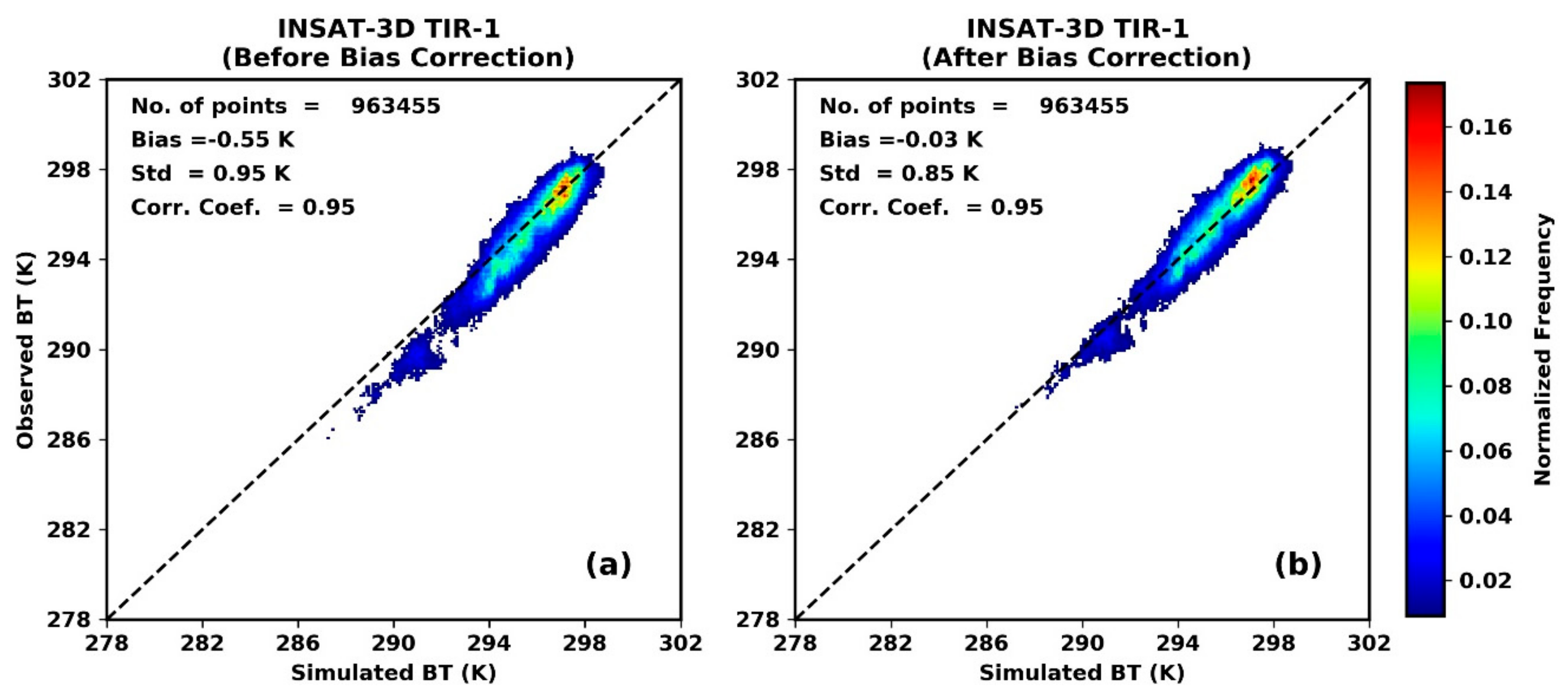
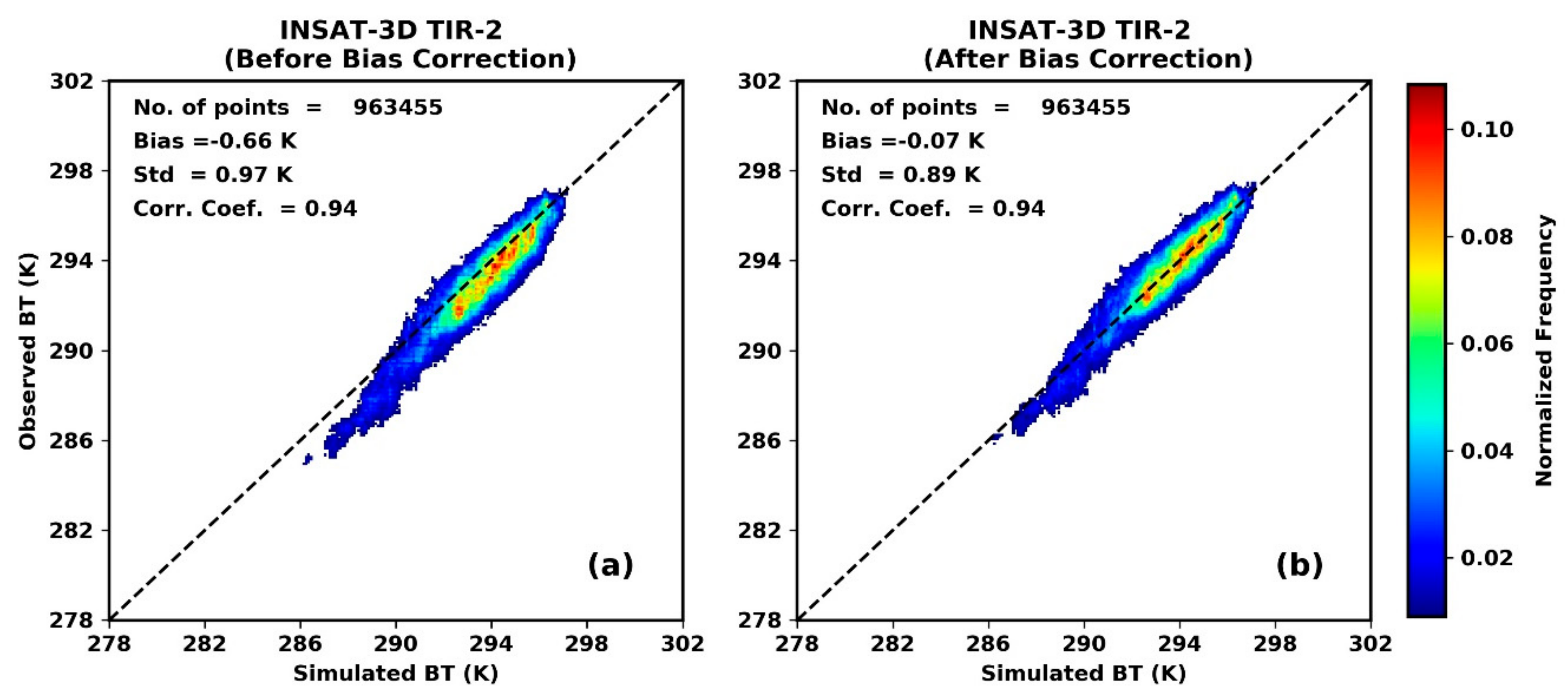
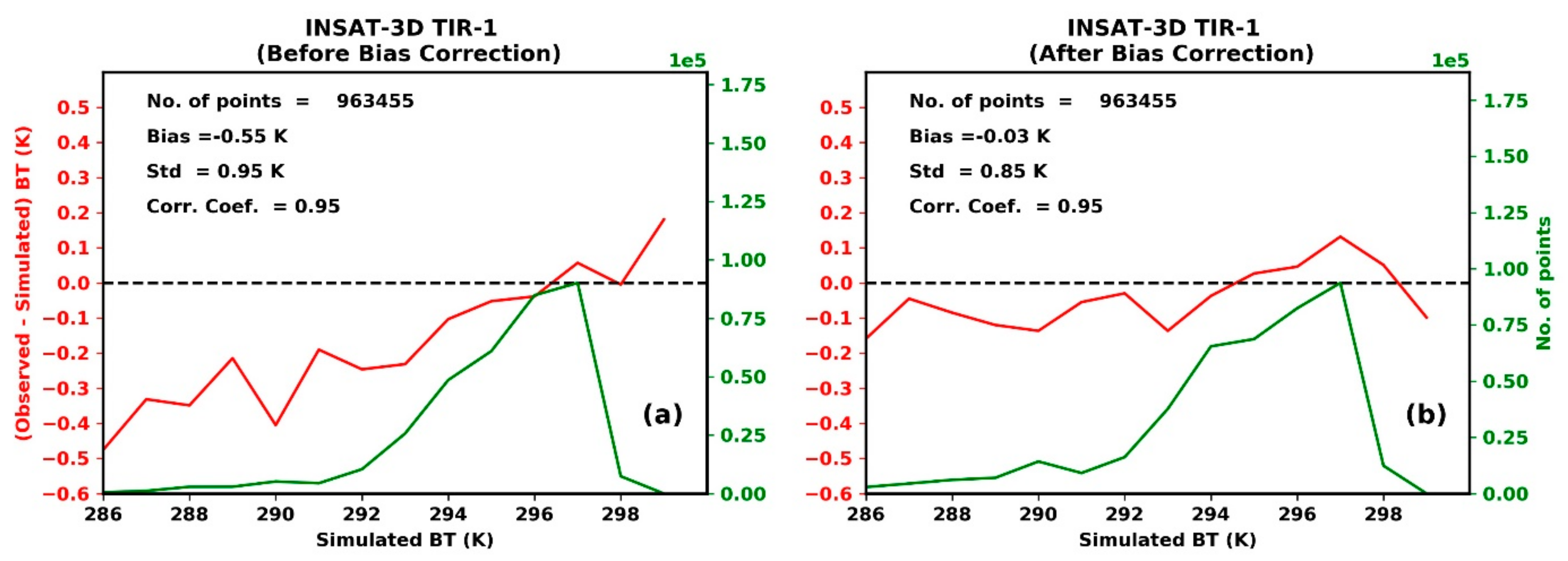
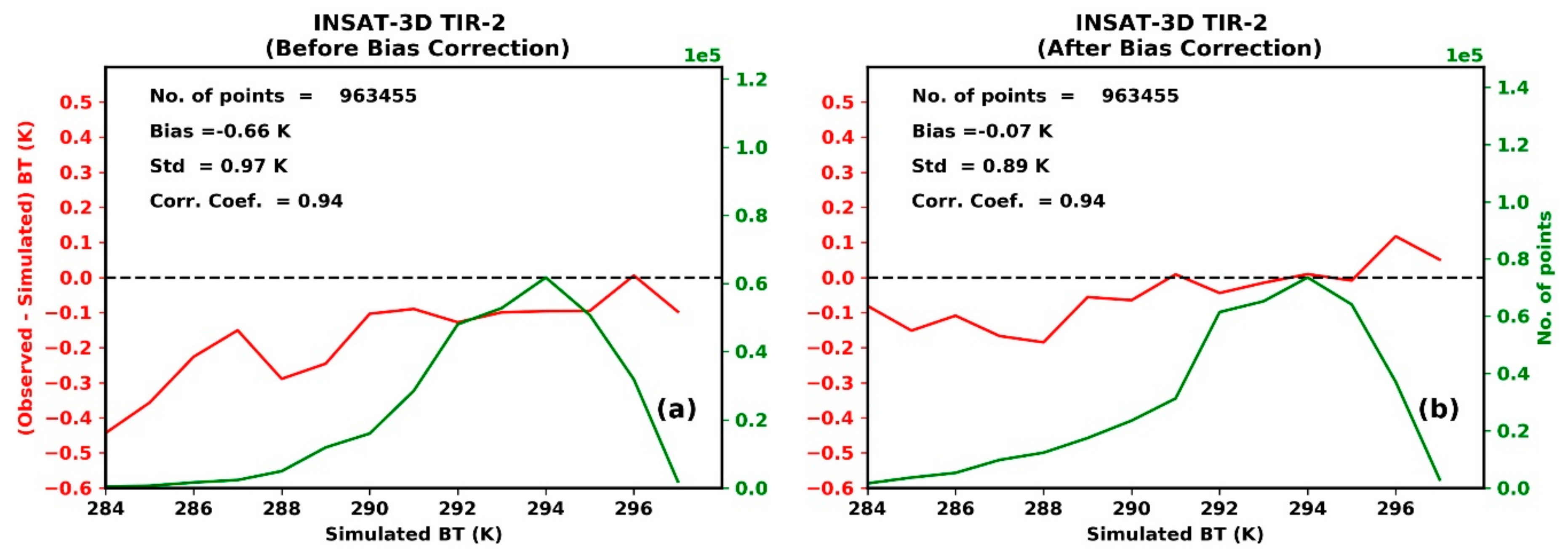
3.2. Bias Correction of the Observations

The satellite observations must be well calibrated and unbiased prior to their use in the retrieval algorithms [34]; otherwise, it will lead to erroneous and biased retrievals. The INSAT-3D/3DR observations, being used in the present study, reported to have shown biases and thereby undergone bias removal using Geostationary Satellite Inter-Calibration System (GSICS) procedures [48]. The biases are computed with reference to observations from hyperspectral sounders such as Advanced Infrared Sounder (AIRS) and Infrared Atmospheric Sounding Interferometer (IASI). Since both of these reference satellites take measurements from LEO platform, a limited matchup dataset could be obtained between these reference instruments and INSAT-3D/3DR, typically twice a day. Because of this, the diurnal biases could not be removed from GEO observations. Therefore, even after GSICS calibration correction, biases persist in the INSAT-3D/3DR observations [48]. Moreover, there is a large bias/uncertainty present in the INSAT-3D/3DR observations during local midnight. Hence, it is further necessary to remove these remaining biases before utilizing them in the retrieval algorithms.

For each satellite acquisition, the actual observations are matched with concurrent simulated observations. The simulations are performed using a fast radiative transfer model RTTOVv11.3, with input data of surface and atmosphere from the nearest available forecast from GFS. The matching of the cumulative density function (CDF) has been utilized here. At first, CDFs of both actual and simulated observations are computed. Thereafter, the actual observations have been mapped according to the simulated CDF to get the corrected observations. A typical example of bias correction procedure applied on INSAT-3D observations is shown in Figure 1 and Figure 2.

Figure 1 and Figure 2 illustrate the bivariate normalized density plots for TIR-1 and TIR-2 channels before and after the bias correction. It may be noted from these figures that the bias is not constant across the range of values, but is defined by a slope in the best fit. A similar bias correction procedure is also applied on INSAT-3DR channels prior to retrieval. It is interesting to note that the scatter plots for both INSAT-3D/3DR deviate from one-to-one line towards lower SST values, even after bias correction, indicating the cloud-leakage problem arising due to inability of cloud-detection algorithm in removing small fractional cloudy pixels. This might lead to small residual bias in the retrieved SST even after bias correction. This is also supported from Figure 3 and Figure 4 that depict differences in the observed and simulated BT corresponding to different values of simulated BT for TIR-1 (Figure 3) and TIR-2 (Figure 4). These Figure 3 and Figure 4 show that TIR-1 and TIR-2 observations have negligible bias around 296 K, which increases towards colder BTs, with values of −0.4 K at 286 K (284 K) for TIR-1 (TIR-2). The bias correction procedure brings these bias values within ±0.1 K, which is a significant improvement. The small residual trend in the bias may be due to the distribution of BT values largely concentrated over 297 K (294 K) for TIR-1 (TIR-2). This needs further improvement in future by applying better cloud filtering procedures, e.g., [22], and utilizing pooled dataset for longer duration instead of just a single acquisition. Another reason for the residual bias may be the zenith angle dependency of the forward RT model, cf. [49].

3.3. NLSST Algorithm

The NLSST algorithm has been proposed by Walton [35], in which the weighting factor for atmospheric correction is assumed proportional to a first-guess SST value that can be obtained in various ways. For SST estimation, the following form of the NLSST algorithm was used in this study

$$SST=a_0+a_1{T}_1+a_2\left(\sec \mathsf{\theta }-1\right)+a_3{T}_{sfc}.\left(T_1-T_2\right)+a_4\left(\sec \mathsf{\theta }-1\right).\left(T_1-T_2\right))$$

(1)

where T₁ and T₂ are the BTs of INSAT-3D/3DR thermal IR channels (TIR-1 and TIR-2) and θ is the satellite zenith angle. a₀, a₁, a₂, a₃ and a₄ are the retrieval coefficients estimated from the regression analysis using collocated/simulated BT observations from satellite and SST measurement. T_sfc is the a priori estimate of SST taken from the GFS model forecast.

The atmospheric profiles and required surface variables have been obtained from the ECMWF diverse data set [50]. The simulations have been performed using RTTOV-v11.3 for the clear atmosphere over oceanic regions spanning from 0°E–130°E and 60°S–60°N only, corresponding to the full disk-viewing region of INSAT-3D/3DR and for satellite zenith angle varying from Nadir up to 60 degrees.

Currently, Equation (1) is being used operationally to retrieve SST from INSAT-3D/3DR Imagers at MOSDAC/SAC and MMDRPS/IMD. However, real-time bias correction is not being applied on satellite observations in operational SST retrieval.

3.4. 1DVAR Algorithm

The relationship between geophysical parameter and satellite measurements can be written in a generalized form as

$$\mathit{y}=\mathit{F}\left(\mathit{x}\right)+e$$

(2)

where y is the measurement vector (satellite observations), F(x) is the non-linear forward model (radiative transfer (RT) model) which transforms x, the state vector containing the relevant geophysical parameters of the ocean and the atmosphere, into measurement vector [51]. e is a residual uncertainty term containing uncertainties of measurement and the forward model.

The forward model, i.e., RT model synthesizes the top-of-atmosphere BTs that should be measured by the individual channels of a radiometer given prior knowledge of the relevant atmosphere state and surface condition (x). Here, a fast RT model RTTOV11.3 has been used as the forward model.

Now, by inverting Equation (2), we can retrieve the most likely geophysical parameters (x) that can reproduce the top-of-the-atmosphere brightness temperatures, y. Herein, we have used an inverse approach (1DVAR or optimal estimation (OE)) developed by Rodgers [51] for retrieving the x (e.g., SST).

Assuming the forward model is a general function of the state, the representative (measurement + model) error has a Gaussian distribution, and there is a prior estimate with a Gaussian uncertainty distribution, the maximum probable state x can be found by minimizing the cost function, J

$$J\left(x\right)={\left(x-x_0\right)}^T{B}^{-1}\left(x-x_0\right)+{\left(y-y\left(x\right)\right)}^T{R}^{-1}\left(y-y\left(x\right)\right)$$

(3)

where y is the observations with error covariance R; x₀ being the prior atmospheric state having error covariance B and y(x) is the observations simulated through the forward model using atmospheric state x.

Rodgers [52] has given the following iterative solution for the minimization of J(x)

$$x_{n+1}=x_0+B{H}_n^T{\left(H_{n}B{H}_n^T+R\right)}^{-1}\left[y-y\left(x_n\right)-H_n\left(x_0-x_n\right)\right]$$

(4)

where x_n being the n^th estimate of atmospheric state, x₀ is the background atmospheric state. y represents the actual BTs of concerning channels and y(x_n) are the simulated BTs corresponding to n^th atmospheric state (x_n). H_n is the sensitivity of the simulated observations with respect to state variables, also known as the Jacobian matrix. H_n consists of the partial derivatives of the BTs in a particular channel with respect to each parameter of the state vector (x_n). Due to nonlinearity, these partial derivatives need to be computed at each iteration (state).

The Equation (4) implies that the sensitivity information (H_n) together with the difference between the actual BTs, y, and the simulated BTs, y(x_n), can be used to estimate the difference between the prior information about the state and the actual state, and thereby to estimate the actual state.

3.4.1. 1DVAR Setup

In our case, the BTs of thermal IR split-window channels from INSAT-3D/3DR Imagers are used as measurement vector, y, in the forward model. The prior information is taken from GFS forecast fields which provide the temperature (t) and humidity (q) values at 25 atmospheric pressure levels starting from 1000 hPa to 1 hPa along with the surface temperature (equivalent to SST over the ocean and LST over the land) and surface air temperature/humidity. We have assumed forecast temperature and humidity profiles including SST as state vector (x_n), i.e., x = [t(1:25), SST, q(27:51)]. The state vector x hence consists of 51 geophysical parameters. The error covariance matrix B of the a priori atmospheric state therefore, has 51 × 51 elements, in which temperature and humidity are assumed mutually uncorrelated. The error covariance of all the parameters is calculated by comparing the forecast fields with corresponding analysis fields. To prepare an error covariance matrix, B, the entire year of forecast and analysis fields from GFS is considered. In case of SST, the standard deviation of the error is found to be 0.51 K.

For simulating the top-of-the atmosphere BTs, the full atmospheric state has been used. The measurement covariance matrix, R, is set to a 2 × 2 diagonal matrix corresponding to TIR-1 and TIR-2 channels. The uncertainty of each channel is considered as per respective noise equivalent differential temperature (NEDT) values, i.e.,

$$R=\left[\begin{array}{cc}{e}_1^2& 0\\ 0& e_2^2\end{array}\right]$$

where e₁ = 0.15 K and e₂ = 0.25 K as given in Table 1. At present, for providing more weight to the observations, the RT model errors have been ignored. However, these may be suitably modified in the operational implementation of the algorithm after due sensitivity study.

Now, using the values of H, B and R in iterative solution (Equation (4)), the actual atmospheric state is retrieved. Although the retrieved atmospheric state includes temperature and humidity profiles, the measurement vector consists of channels that are insensitive to these profiles. The channels in the measurement vector are most sensitive to the underlying surface; therefore, SST is only considered as the final retrieved parameter.

3.4.2. Convergence Testing

The atmospheric state, for which the solution of Equation (4) converges, would be the optimized or final retrieved state. To check whether the solution is actually being converged or not, can be ensured through the minimization of the cost function, J [52]. The minimization of the cost function can be performed by examining the change in the cost function (ΔJ = J_i − J_i+1) between two subsequent iterations. For convergence, ΔJ must be decreasing for each subsequent iteration. If ΔJ changes by less than 2%, it is considered that the solution has converged to its final state. In other cases, where there is no decreasing trend in ΔJ, it implies that the solution failed to converge.

4. Results

Assessment of both the algorithm’s skill has been performed through the validation of the retrieved SST products against the reference SST values, i.e., iQuam SST products. The extensive validation of the retrieved SST is carried out by comparing it for a six-month’s period spanning from December 2019 to May 2020. The period embodies different seasons, i.e., winter, spring and summer, thereby, covering maximum variability of the SST. The monsoon season, June–September, is not considered as during this time the Indian Ocean is dominated by the cloud cover. The first guess SST, henceforth denoted by FCT, is also compared with the reference SST to monitor the impact of actual observations in the retrievals. A typical example of daily composite SST retrieved from INSAT-3D and 3DR Imagers for the day 07 January 2020 is shown in Figure 5. For better comparison, a daily averaged forecast SST on the same day, which was used as the first guess and for bias correction, is shown in Figure 6.

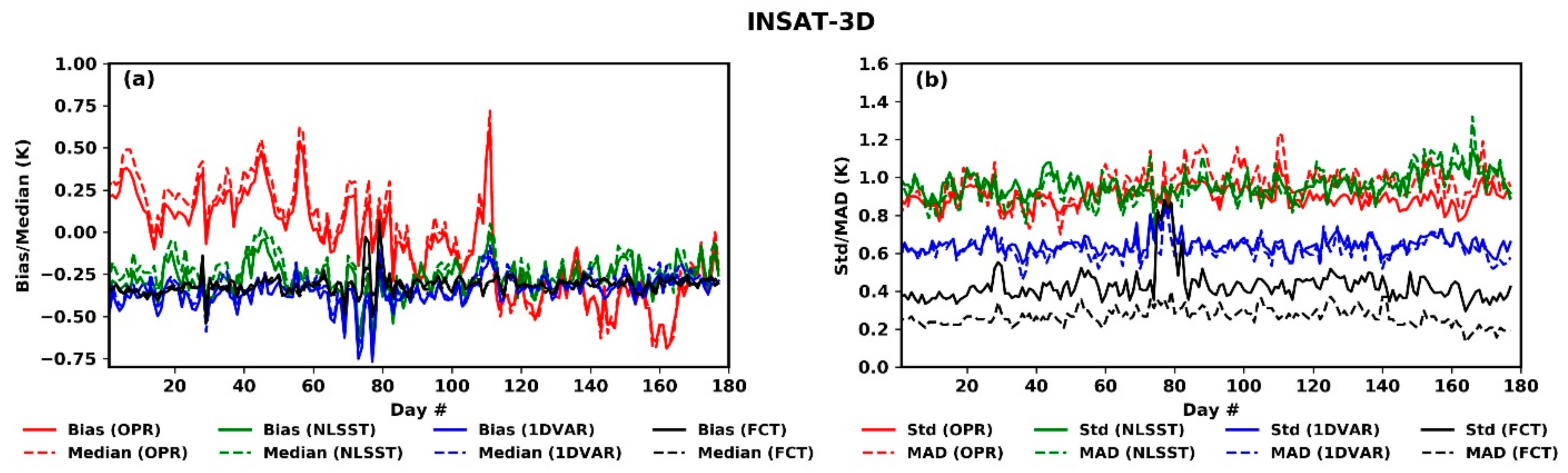
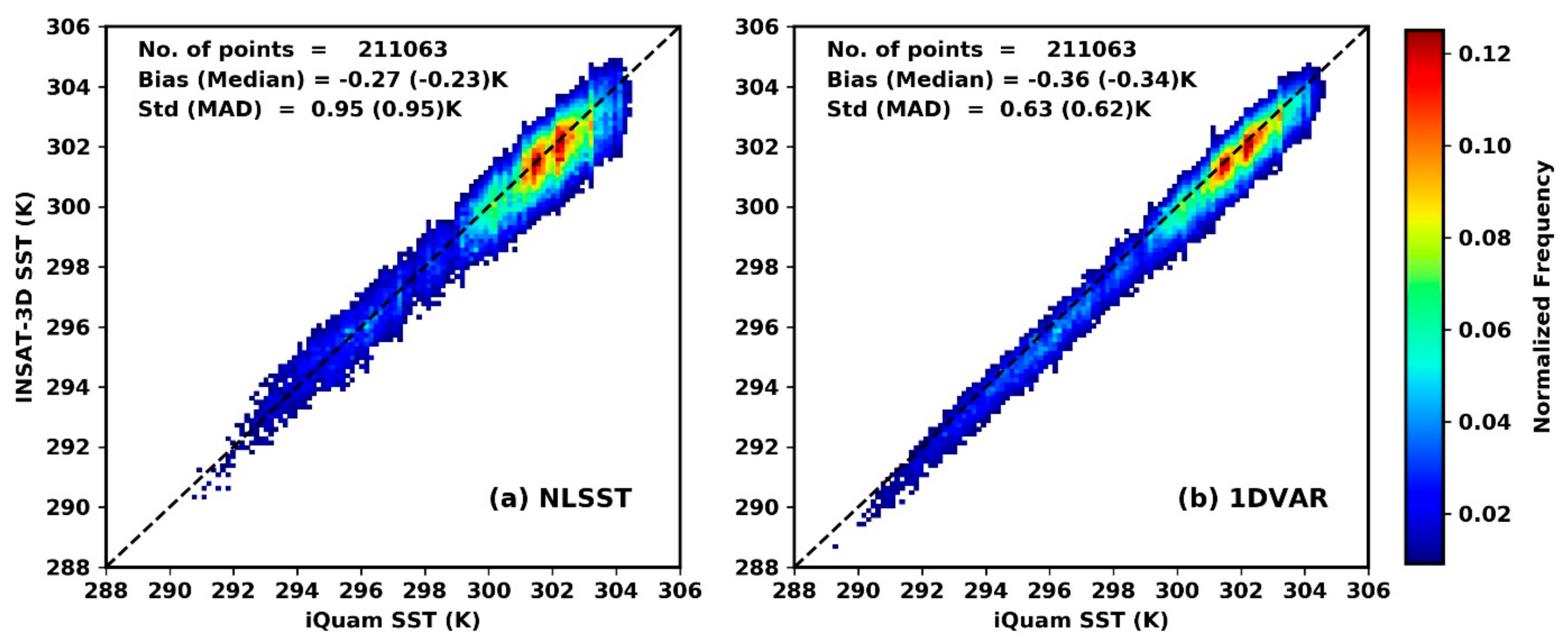
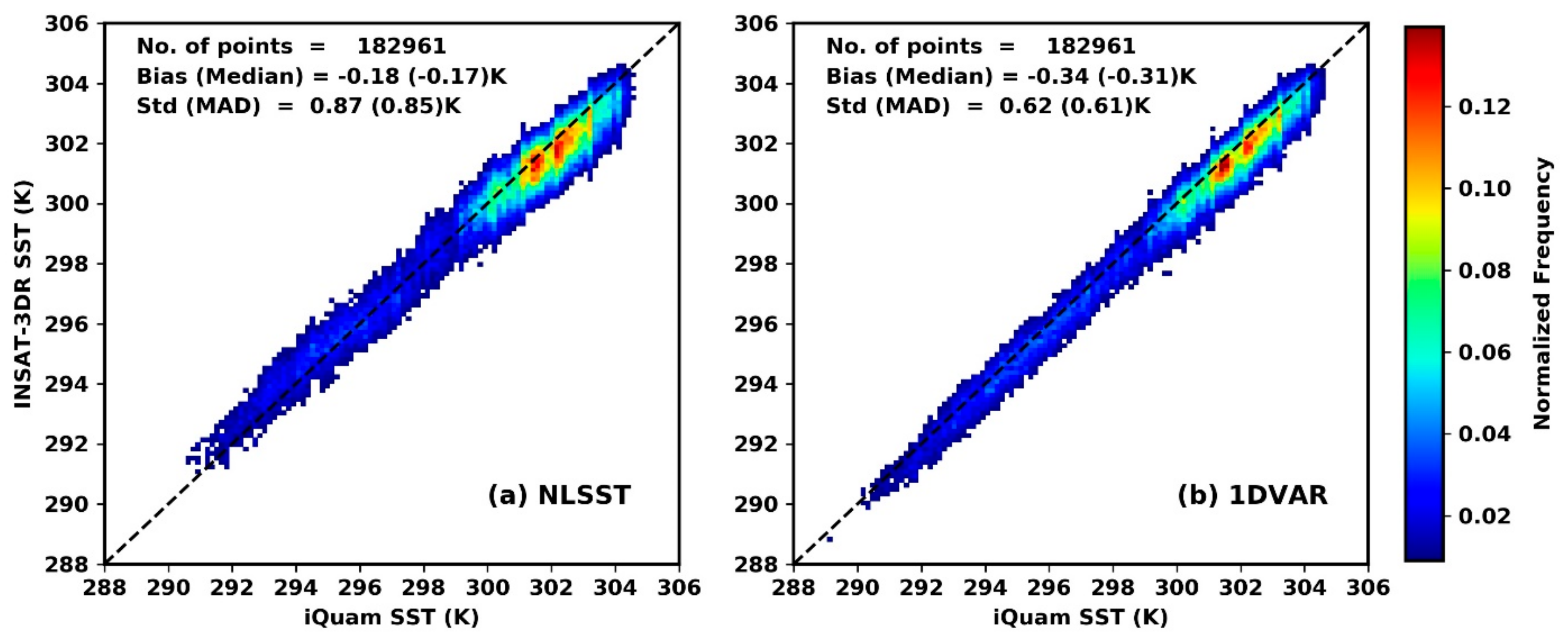
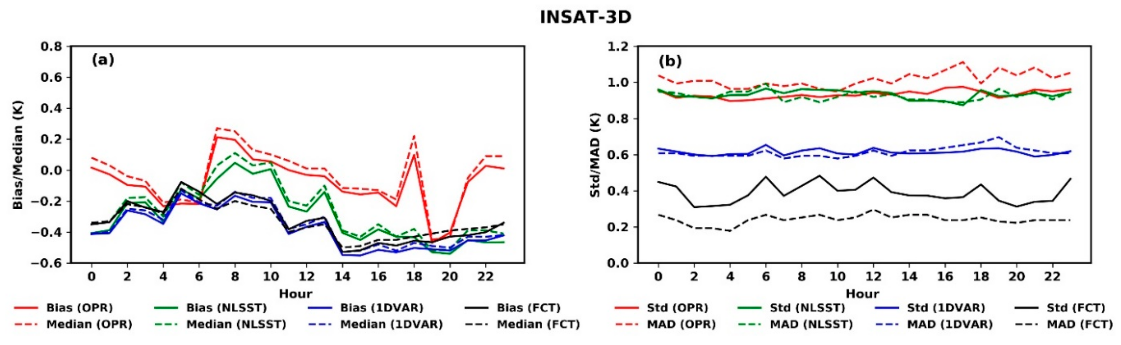
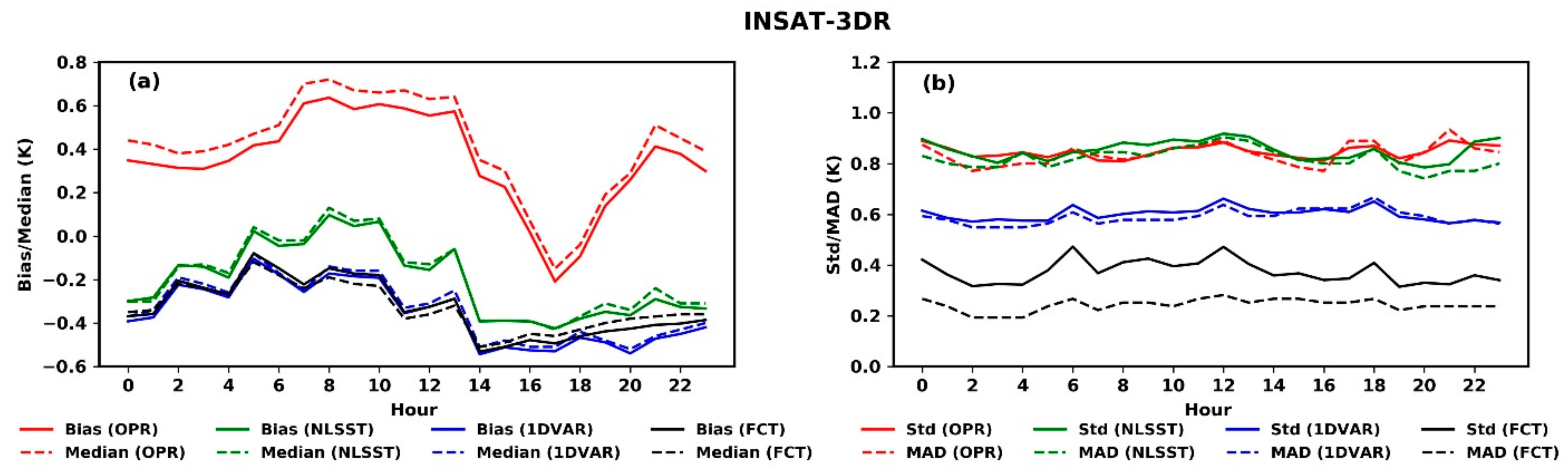
4.1. Validation Against iQuam SST Measurements

For comparing the SST products retrieved using both the algorithms, first they have been collocated with iQuam SST data to generate the matchup dataset. For collocation, the spatial resolution of 0.04° (corresponding to the INSAT-3D/3DR resolution and spatial sampling of retrieved SST) and temporal window of ±15 minutes is assumed. The standard statistical quality indicators, like bias (Bias), standard deviation (Std) and Pearson correlation coefficient for SST retrieved from INSAT-3D/3DR using both the algorithms are calculated from the reference SST. As we know that Bias and Std do not account for outliers present in the data, these indicators may sometimes be misleading [53]. Hence, the robust parameters like median (Median) and median absolute deviation (MAD) [53] are also computed to monitor the robustness of the retrieved SST products. These quality indicators are shown in Figure 7 and Figure 8 for INSAT-3D and INSAT-3DR, respectively.

Although Figure 7 and Figure 8 are showing all four-quality indicators, viz., Bias, Std, Median and MAD computed on daily-scale for the six months, the collocation is performed on an instantaneous SST basis and not on the daily-averaged SST. For making MAD comparable to Std, we have multiplied MAD by a factor of 1.4826, cf. [53]. The scale factor is computed with the assumption that the concerned data distribution is Gaussian.

It can be observed from Figure 7 that Bias and Median do not show any noteworthy difference, so as Std and MAD. This implies the robustness of the matchup data. We can further observe that the 1DVAR shows the higher accuracy (0.6 K) than the NLSST (0.9 K). However, both algorithms are showing negative biases, i.e., underestimating SST values as compared to iQuam SST. Moreover, the performance of the 1DVAR is more consistent than the NLSST throughout the period, demonstrating superior efficacy of the 1DVAR over the NLSST. A point worth mentioning here is that for the overall period the biases in SST derived from the NLSST (−0.27 K in INSAT-3D and −0.18 K in INSAT-3DR) are smaller compared to the 1DVAR SST (−0.36 K in INSAT-3D and −0.34 K in INSAT-3DR). It may be noted that the NLSST and the 1DVAR SST are skin SST without any correction for bulk-skin SST, whereas the iQuam SST is the representative of subsurface or bulk SST. Therefore, the bulk-skin SST correction of −0.2 K needs to be applied on the retrieved skin SST [54]. This means that the effective biases in the retrieved SST should be around −0.07 K (0.02 K) in the NLSST and −0.16 K (−0.14) in the 1DVAR for INSAT-3D (INSAT-3DR). It may be further noted that the INSAT-3D/3DR Imager observations undergo large biases and uncertainties during the satellite eclipse period (peak midnight sun/stray-light problem) as discussed in Shukla and Thapliyal [48]. This leads to the large bias/uncertainties in the operational SST (OPR) products presently available from INSAT-3D/3DR.

As discussed by Merchant [34] this improvement in the 1DVAR SST in comparison to the NLSST is because it utilizes an accurate prior SST information as the first guess. It is interesting to note that when FCT SST is compared with iQuam for the same duration, it showed the value of Std < 0.5 K. It can be explained from the fact that in-situ measurements are utilized to improve the initial conditions in NWP models. Therefore, as 67% of the information content is attributed to the first guess [34], the overall Std of the 1DVAR is significantly smaller than the NLSST. The NLSST has higher Std due to the fact that the satellite observations impart the full information content for the retrieval. Although FCT SST has shown the smallest error (Std) than the SST derived from the NLSST and 1DVAR algorithms, it lacks the small-scale SST features like thermal gradients, due to the coarser spatial resolution (50 km) and significant smoothing.

To monitor the error distribution, the matchup dataset is divided into two categories as follows:

• $\left|SS{T}_{1DVAR}-SS{T}_{iQuam}\right|\le 1K$ Filtered data referred to hereafter as FILT_DATA.
• Entire matchup, referred to hereafter as NOFILT_DATA.

The validation statistics on a monthly scale for these two categories of dataset is shown in

Table 2. Monthly Validation Statistics of INSAT-3D (FILT_DATA shown in bracket).

Month	No. of Matchups (% of total)	CC *	Bias (K)	NLSST Median (K)	Std (K)	MAD (K)	CC *	Bias(K)	1DVAR Median (K)	Std (K)	MAD (K)
December 2019	54,116 (85.8)	0.97 (0.97)	−0.28 (−0.15)	−0.22 (−0.09)	0.94 (0.86)	0.92 (0.82)	0.99 (0.99)	−0.38 (−0.23)	−0.36 (−0.26)	0.62 (0.48)	0.64 (0.53)
January 2020	34,164 (87.5)	0.96 (0.97)	−0.22 (−0.10)	−0.16 (−0.07)	0.95 (0.87)	0.92 (0.83)	0.99 (0.99)	−0.35 (−0.22)	−0.32 (−0.24)	0.61 (0.47)	0.59 (0.50)
February 2020	37,732 (83.6)	0.96 (0.96)	−0.35 (−0.22)	−0.32 − (0.18)	0.92 (0.86)	0.92 (0.85)	0.98 (0.99)	−0.42 (−0.27)	−0.40 (−0.29)	0.65 (0.46)	0.62 (0.50)
March 2020	32,404 (87.7)	0.96 (0.97)	−0.24 (−0.13)	−0.23 (−0.13)	0.93 (0.87)	0.93 (0.86)	0.98 (0.99)	−0.33 (−0.21)	−0.32 (−0.23)	0.62 (0.49)	0.62 (0.53)
April 2020	28,877 (87.3)	0.96 (0.98)	−0.27 (−0.17)	−0.25 (−0.15)	0.94 (0.88)	0.96 (0.90)	0.99 (0.99)	−0.32 (−0.20)	−0.30 (−0.23)	0.62 (0.49)	0.62 (0.53)
May 2020	23,770 (87.9)	0.98 (0.98)	−0.22 (−0.10)	−0.18 (−0.07)	1.02 (0.95)	1.05 (0.96)	0.99 (0.99)	−0.30 (−0.19)	−0.27 (−0.19)	0.63 (0.49)	0.62 (0.53)
Overall	211,063 (86.5)	0.97 (0.9)	−0.27 (−0.15)	−0.23 (−0.12)	0.95 (0.88)	0.95 (0.86)	0.99 (0.99)	−0.36 (−0.23)	−0.34 (−0.25)	0.63 (0.48)	0.62 (0.52)

* CC: Pearson correlation coefficient.

and

Table 3. Monthly Validation Statistics of INSAT-3DR (FILT_DATA shown in bracket).

Month	No. of Matchups (% of total)	CC *	Bias (K)	NLSST Median (K)	Std (K)	MAD (K)	CC *	Bias (K)	1DVAR Median (K)	Std (K)	MAD (K)
December 2019	40,286 (87.4)	0.97 (0.98)	−0.26 (−0.15)	−0.21 (−0.11)	0.83 (0.76)	0.79 (0.71)	0.99 (0.99)	−0.36 (−0.23)	−0.33 (−0.25)	0.60 (0.46)	0.59 (0.50)
January 2020	27,602 (88.3)	0.98 (0.98)	−0.22 (−0.14)	−0.20 (−0.13)	0.73 (0.68)	0.77 (0.71)	0.99 (0.99)	−0.37 (−0.26)	−0.36 (−0.28)	0.58 (0.46)	0.58 (0.50)
February 2020	32,486 (85.7)	0.97 (0.98)	−0.24 (−0.15)	−0.22 (−0.13)	0.73 (0.67)	0.74 (0.70)	0.98 (0.99)	−0.42 (−0.27)	−0.39 (−0.29)	0.61 (0.45)	0.59 (0.49)
March 2020	31,578 (87.7)	0.97 (0.97)	−0.20 (−0.10)	−0.19 (−0.10)	0.90 (0.84)	0.87 (0.82)	0.99 (0.99)	−0.35 (−0.23)	−0.33 (−0.25)	0.61 (0.47)	0.59 (0.50)
April 2020	29,428 (88.7)	0.98 (0.98)	−0.08 (0.01)	−0.10 (−0.01)	0.97 (0.91)	0.95 (0.89)	0.99 (0.99)	−0.25 (−0.14)	−0.22 (−0.15)	0.63 (0.49)	0.61 (0.53)
May 2020	21,581 (87.4)	0.98 (0.98)	−0.04 (0.08)	−0.02 (0.09)	1.07 (1.00)	1.13 (1.04)	0.99 (0.99)	−0.23 (−0.12)	−0.19 (−0.12)	0.65 (0.50)	0.65 (0.56)
Overall	182,961 (87.6)	0.98 (0.98)	−0.18 (−0.09)	−0.17 (−0.09)	0.87 (0.81)	0.85 (0.79)	0.99 (0.99)	−0.34 (−0.21)	−0.31 (−0.23)	0.62 (0.47)	0.61 (0.52)

* CC: Pearson correlation coefficient.

for the INSAT-3D and 3DR, respectively.

In Table 2, the validation statistics corresponding to the first category is provided in the small parenthesis. Based upon the parameters’ values, the following inferences can be drawn:

• The majority of the matchup dataset (>85%) is lying within 1 K of iQuam SST, leaving only <15% of it beyond this limit.
• Bias and Median do not show much difference indicating the robustness of the matchup data. The same outcome is endorsed by Std and MAD values being almost similar.
• For a larger population of the data, the 1DVAR SST shows Std (Bias) of 0.48 K (−0.23 K) whereas the NLSST gives 0.88 K (−0.15 K). However, SST accuracy with 0.95 K (−0.27 K) for the NLSST and 0.63 K (−0.36 K) for the 1DVAR, degrades slightly for the entire matchup. These values are without bulk-skin SST correction.
• The 1DVAR produces SST with greater accuracy and consistency than the NLSST, clearly seen when validated against iQuam SST.
• Both the algorithms demonstrate the consistent performance for all months, thereby ensuring their robustness.

Similarly, Table 3 illustrates the monthly validation statistics for SST retrieved from INSAT-3DR observations. Except for a few differences, the validation statistics are more or less similar for SST retrieved from both the satellites, INSAT-3D/3DR. In the INSAT-3DR, the NLSST performs slightly better showing Std (Bias) of 0.87 K (−0.18 K) than in the INSAT-3D when observed for the entire dataset. However, the 1DVAR exhibits similar error characteristics for both INSAT-3D and 3DR SST.

To evaluate performance of both algorithms corresponding to different SST values, a bivariate normalized density is computed from the entire dataset (December 2019 to May 2020). Figure 9a,b, respectively, show bivariate normalized density plots for INSAT-3D SST retrieved using the NLSST and the 1DVAR algorithms. Here, the bivariate density states the number of SST pairs (retrieved and iQuam SST) in a given bin of SST values. If the same number of values from both SSTs lies in a given bin this implies there exists a strong agreement between them. The parameters, viz., total number of matchup points, bias, median, Std and MAD, are also given in the respective plots.

From these plots, it is evident that most of the matchup data are concentrated over the higher SST (>298 K) values. It can also be inferred that both retrieved and iQuam SST are matching well with each other for the entire dynamic range of SST. When observing the spreads around the one-to-one line, it can be seen that the NLSST has a larger spread than the 1DVAR. This implies the higher values of Std (0.95 K) in the NLSST than in the 1DVAR (0.63 K). However, the mean values (Bias) of differences in the NLSST (−0.27 K) is smaller than in the 1DVAR (−0.36 K). Overall, the 1DVAR outperforms the NLSST in terms of both accuracy and consistency of the retrieved SST.

As it can be observed in Figure 10a,b, the INSAT-3DR also demonstrates the similar type of bivariate density pattern. Here too, the density plots are reflecting the improved performance of the 1DVAR over the NLSST. However, the NLSST is providing slightly better results for INSAT-3DR than INSAT-3D, showing the Std value of 0.87 K reduced from 0.95 K. The bias is also reduced considerably from −0.27 K to −0.18 K.

The validation exercise performed for INSAT-3D and 3DR derived SST against iQuam SST implies that the 1DVAR outperforms the NLSST algorithm. The majority of the matchup data (>85%) demonstrate that the retrieval accuracy (Std) is better than 0.5 K in case of the 1DVAR algorithm whereas <0.9 K in the NLSST. The consistent performance of both the algorithms across all months reflects their robustness. The NLSST provides slightly higher accuracy when applied on the observations of INSAT-3DR than INSAT-3D.

Scatter/density plots of the retrieved SST for both INSAT-3D/3DR using the NLSST and the 1DVAR algorithm show that there is a slight shift in the scatter from the one-to-one line mostly representing cooler SST in the INSAT-3D/3DR. This is probably because of the cloud-leakage arising due to retention of the small fractional cloudy pixel as clear-sky pixel in the present cloud detection routine, which will be a key focus area in future work.

The major advantage of the present algorithms is a real-time bias monitoring using RT model simulation of satellite radiances/BTs with inputs from forecast surface temperature (SST) and atmospheric profiles. This is thought to be a plausible solution for correcting the diurnal biases in the GEO satellite observations arising primarily due to stray-light problem at local midnight (~18–20 UTC for INSAT-3D/3DR), which is more severe during satellite eclipse period, i.e., around 23 March and 23 September every year.

To examine the improvement in the diurnal biases in INSAT-3D/3DR using new algorithms, the statistics are generated for hourly binned matchup dataset, and are shown in the Figure 11 and Figure 12 for INSAT-3D and INSAT-3DR, respectively.

From Figure 11 and Figure 12, it is evident that the OPR SST (NLSST without diurnal bias correction) exhibits very high and erratic diurnal variation of biases, particularly around local midnight. Also, it may be kept in mind that there is still a cold bias of around 0.2 K in all the curves, as the reference data are bulk SST from iQuam, thereby, a shift of 0.2 K upward is needed in the bias curves. It is apparent that the new algorithms for INSAT-3D/3DR, i.e., the NLSST and the 1DVAR, are following patterns of FCT in the diurnal variation with the 1DVAR very close to FCT and the NLSST slightly larger at many times of the day. Overall, the 1DVAR followed by the NLSST have smaller biases as compared to the presently operational version of the NLSST algorithms. The Std/MAD curves show that patterns are similar throughout the day and have no clear diurnal dependency. This is because the Std/MAD is a manifestation of the noise uncertainty in the satellite observation. Therefore, for the NLSST there is only a small improvement, whereas there is a large improvement in the 1DVAR due to the use of a priori information from forecast, which has a small Std/MAD as compared to in-situ observation. A large smoothing in the NLSST or 1DVAR, similar to the FCT (50 km), is not advisable, because these satellite observations are primarily used for various applications where high spatial resolution is required.

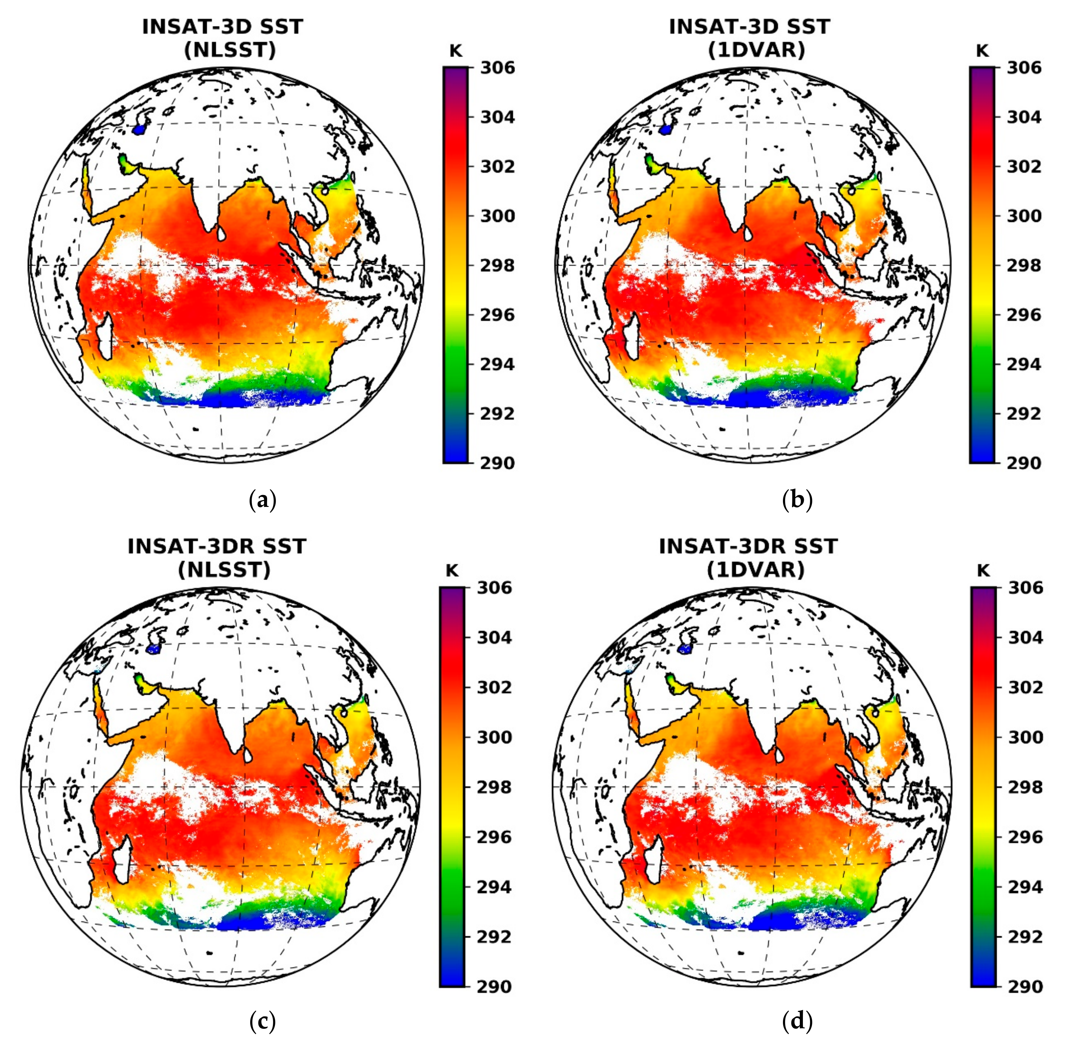
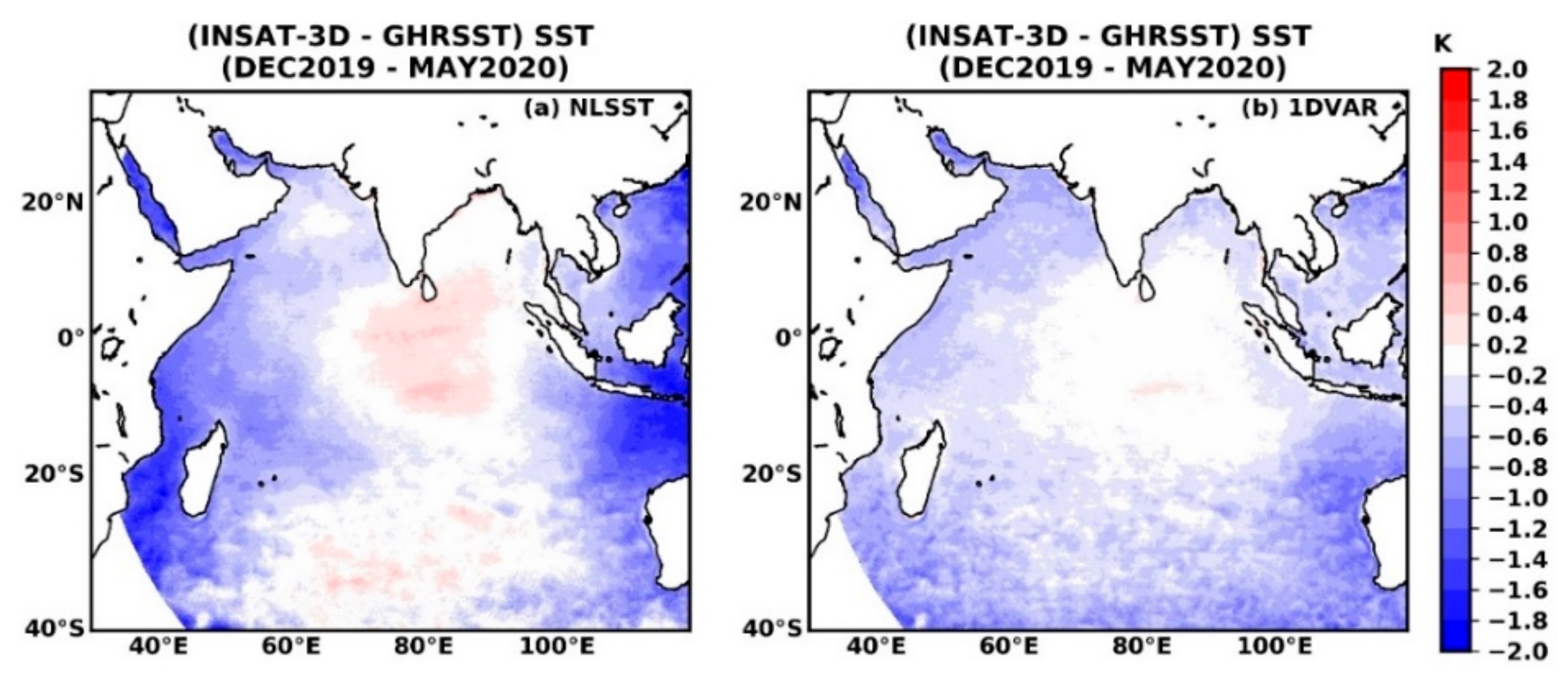
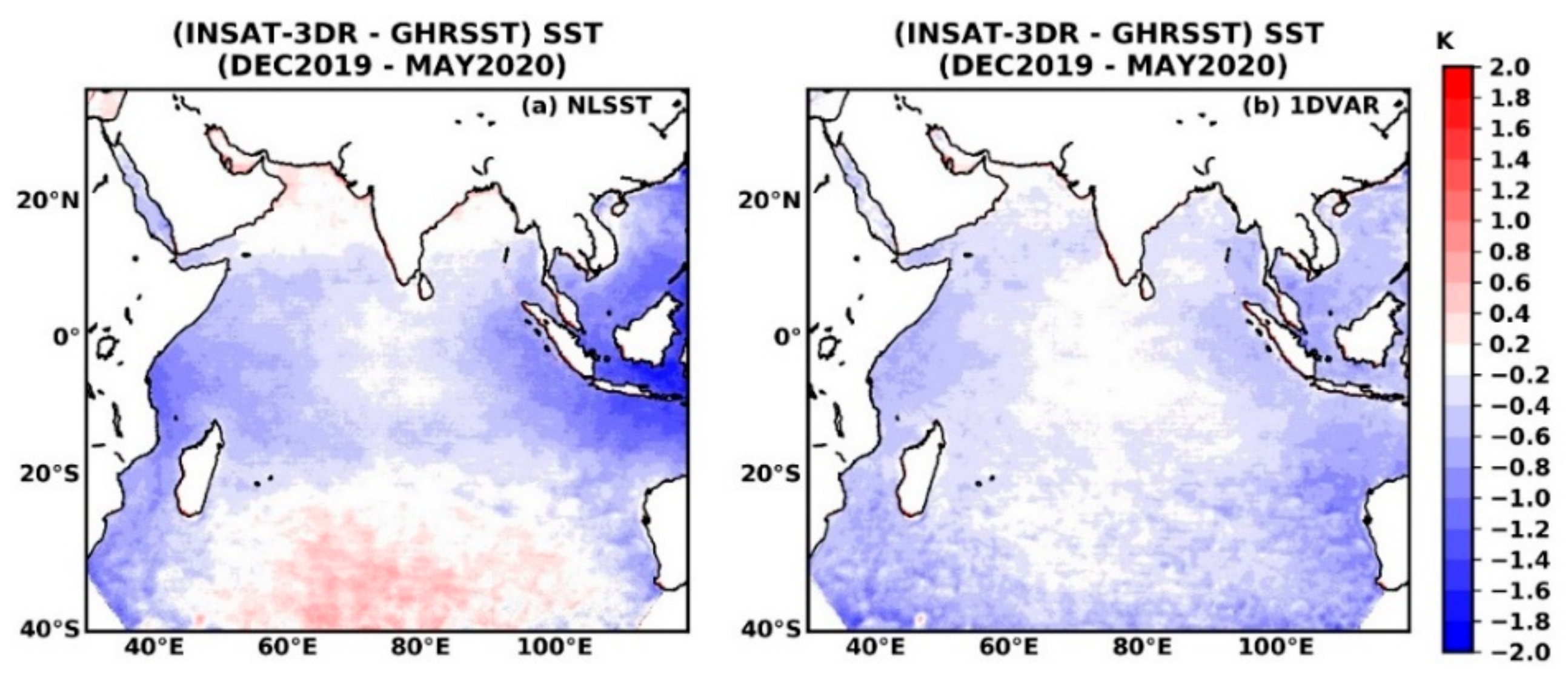
4.2. Comparison with MUR Level-4 Daily Analysis GHRSST Products

To monitor the geographical distribution of errors in the retrieved SST, the difference between retrieved and MUR level-4 GHRSST products are computed for the entire study period. Since MUR level-4 GHRSST is the daily analysis SST as discussed in Section 2.4, the daily average of retrieved SST products using the NLSST and the 1DVAR algorithms for INSAT-3D and 3DR Imagers are calculated. Because of different spatial resolutions of MUR level-4 GHRSST (1km) and INSAT-3D/3DR (4 km), we have resampled both daily products at 5km regular grid. Figure 13 and Figure 14 are showing the difference plots for INSAT-3D and 3DR, respectively. Figure 13a and Figure 14a show that the NLSST has large positive bias in the central Indian Ocean, which changes to negative bias in the eastern and the western Indian Ocean. There is a considerable improvement noticed in the biases over the entire domain using the 1DVAR technique, as shown in Figure 13b and Figure 14b. The negative bias towards peripheral regions in the 1DVAR is significantly smaller as compared to the NLSST.

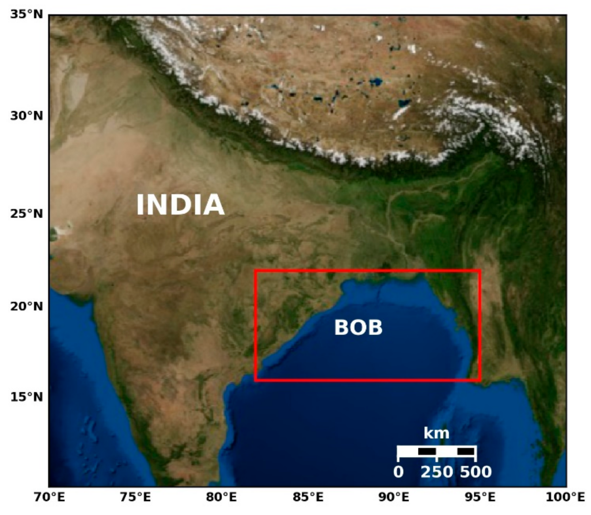
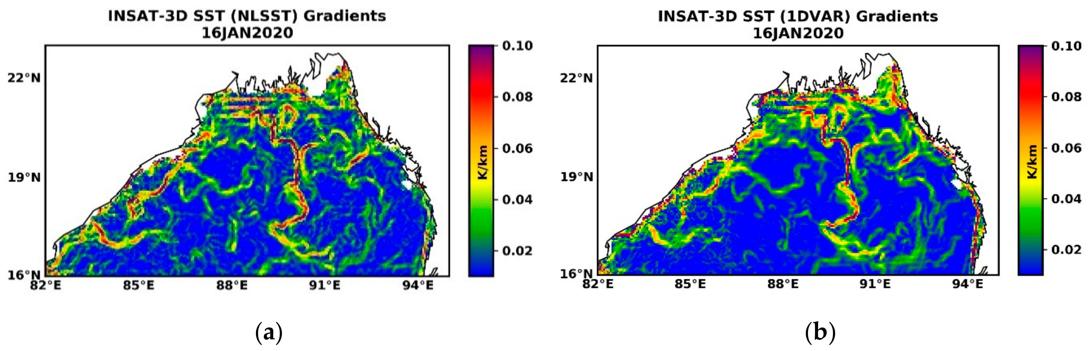
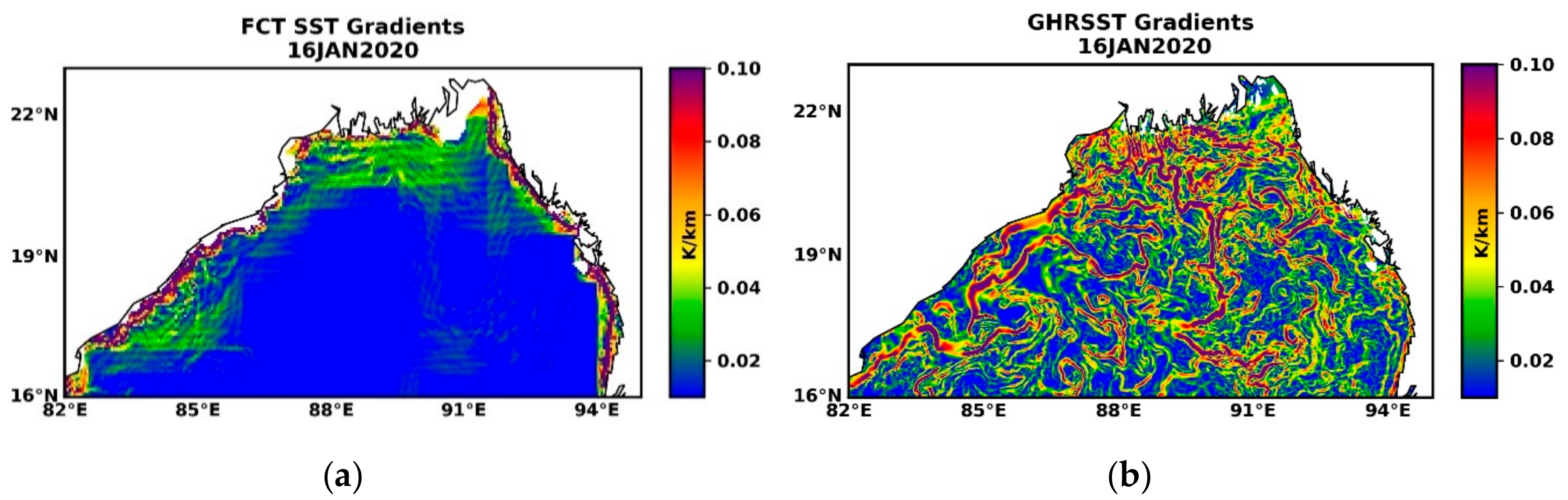
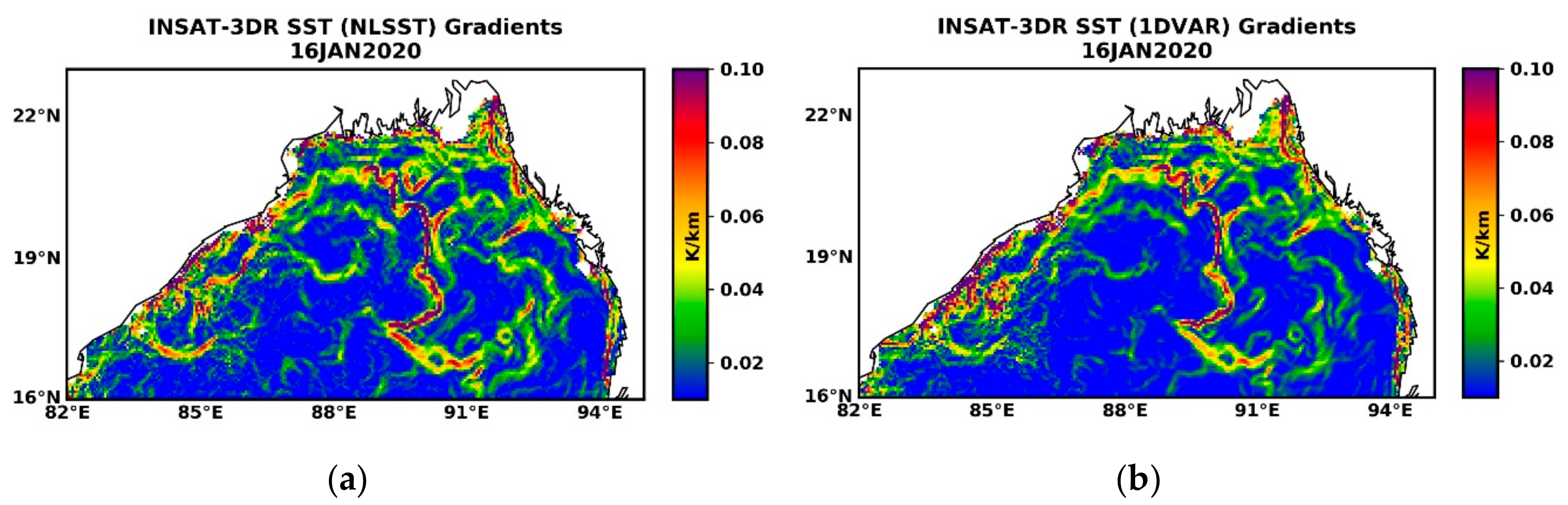
4.3. Thermal Gradients Derived from SST

The spatial gradients of SST, also known as thermal gradients, are primary inputs to predict the potential fishery zones (PFZ) and a major advantage of split-window thermal IR observations from geostationary satellites [43]. Therefore, here we evaluate the thermal gradients observed in the SST retrieved from INSAT-3D/3DR using both the 1DVAR and the NLSST algorithms. These gradients are computed from the daily composite of retrieved SST. The spatial gradients are calculated using central differences in the interior points and one-sided (forward or backward) differences at the boundaries [55]. For the comparison and assessment, the gradients of MUR level-4 GHRSST daily analysis SST products are also shown over the Bay of Bengal (BOB) region (Figure 15). For example, Figure 16a,b illustrate the thermal gradients for INSAT-3D SST estimated using the NLSST and the 1DVAR algorithms for 16 January 2020, respectively. This date was chosen due to the least presence of cloud cover to obtain the gap-free INSAT-3D/3DR SST products. These thermal gradients have been compared with the SST gradients obtained from FCT and MUR level-4 GHRSST, respectively, in Figure 17a,b. Similarly, the thermal gradients derived from the INSAT-3DR SST products are shown in Figure 18a,b. Here, it may be noted that the spatial resolution of FCT is 50 km, whereas the same is 1 km in MUR level-4 GHRSST products, and 4 km in INSAT-3D/3DR products. As gradients are fine scale features, they are observed best in the high-resolution SST products and diffuse as spatial resolution becomes coarser.

From the Figure 16, Figure 17, Figure 18, it is clearly observed that FCT SST is not showing any spatial gradients, mainly due to its coarser spatial resolution. This indicates the limitation of FCT SST to utilize it in important oceanographic applications, such as prediction of PFZ. Although FCT SST showed the least bias/Std when compared with iQuam SST (Figure 7 and Figure 8), it lacks the small-scale features of SST. Thereby, the retrieval of accurate SST from satellite observations becomes more important. Moreover, both algorithms proposed in the present study are able to produce SST that depicts all the prominent features of thermal gradients as observed in the MUR level-4 GHRSST products. Since MUR level-4 GHRSST has ultra-high spatial resolution of 1km, it exhibits more gradient features, mostly the weaker ones, as compared to INSAT-3D and 3DR SST products.

5. Conclusions

The motivation of the present study comes from the utility of high spatial and temporal resolution GEO satellite observations for estimating one of the most important boundary parameters over the ocean, i.e., SST. Presently, there are many GEO satellites from various countries populated over the equatorial orbit, providing continuous coverage of the global tropics and mid-latitude regions. Indian GEO satellites, INSAT-3D/3DR, provide coverage over a very important region, i.e., the Indian Ocean. However, so far INSAT-3D/3DR SST products suffer from the midnight stray sunlight problem, adding large uncertainties in the observations. An attempt was made by Ojha and Singh [40] to develop a physical retrieval method, but there were a few shortcomings of the study. For example, they used SST climatology in the RT model for the bias correction of INSAT-3D observations as well as the background/first-guess and used it for the relative assessment of the retrieved products.

In the present study, we have exploited the 1DVAR technique to retrieve the SST using thermal split-window IR observations from INSAT-3D/3DR. The conventional regression-based retrieval technique, NLSST, has also been utilized for SST estimation. Although the NLSST algorithm is already implemented from July 2018 at MOSDAC/SAC and MMDRPS/IMD, it does not have a mechanism to correct for diurnal and seasonal dependent biases. In the present study, this has been corrected using a real-time bias correction of satellite observations using model forecast fields as input in the RT model. Since both the algorithms, NLSST and 1DVAR, utilize RT model for coefficient generation as well as forward/Jacobian computation, this procedure makes satellite observations consistent with the RT model. Both algorithms are tested for six months of INSAT-3D and 3DR observations to retrieve SST to capture seasonal variability ranging from winter (cold SST) to summer (warm SST). The quantitative assessment of the retrieved SST is carried out by validating with the iQuam SST. It may be noted that the validation statistics have been generated for daily and monthly scales using pooled matchup dataset of instantaneous SST fields, and not using the daily/monthly averaged SST that introduces significant smoothing. To monitor the accuracy of the retrieved SST in different SST bins, bivariate density plots are demonstrated. Based on the validation exercise, it has been observed that the 1DVAR outperforms the NLSST for both the satellites. The 1DVAR based retrieval shows a similar accuracy with Std (Bias) of 0.63 K (−0.36 K) for both INSAT-3D and 3DR. Whereas, the NLSST provides slightly less accurate SST with Std (bias) of 0.87 K (−0.18 K) for INSAT-3DR and 0.95 K (−0.27 K) for INSAT-3D, respectively. It may be noted that an additional cold bias of about 0.2 K may also be removed because the satellite SST fields are skin-SST, whereas the iQuam is bulk or sub-skin SST. This brings a bias value in both the 1DVAR and the NLSST very close to 0 that implies a significant improvement in SST retrieval accuracy using the 1DVAR algorithm over the NLSST. Additionally, the majority (>85%) of retrieved SST data lie within 1 K of the reference SST giving the accuracy of <0.5 K in case of the 1DVAR and 0.8 K in case of the NLSST. This may be because the 1DVAR utilizes the accurate a priori FCT SST as the first-guess, which provides about 67% of the information content to the retrieval [34], whereas the NLSST utilizes direct satellite observations, which has large uncertainties.

As the real benefit of a GEO satellite is to provide continuous observations for high spatial and temporal resolution SST, the diurnal pattern of the bias is also evaluated. The present study shows that using real-time bias correction leads to a reduction in the diurnal biases in the OPR SST and brings these biases very close to the biases in the FCT SST. Although the NLSST used herein shows slightly higher biases as compared to the 1DVAR, they are still far superior to the OPR algorithm without any mechanism for diurnal and seasonal dependent bias correction. Moreover, the Std does not exhibit diurnal variation, and is improved significantly in the 1DVAR followed by the NLSST algorithm as compared to the OPR. Other than the validation, the retrieved SST has been further exploited for the application of small-scale features such as spatial thermal gradient studies. The computed spatial thermal gradients from SST retrieved using the 1DVAR and the NLSST algorithms exhibit an excellent match for the large-scale features with the MUR level-4 GHRSST derived gradients. The new 1DVAR and NLSST algorithms are able to capture the majority of the prominent features observed in MUR level-4 GHRSST gradients that is very essential for many oceanographic applications, especially PFZ identification.

In a nutshell, the present work demonstrates that the 1DVAR physical retrieval and the NLSST based algorithms perform very well after making RT model-dependent observation bias correction from closest forecast fields as input to the RT model. These algorithms show far superior accuracy in terms of both diurnal/seasonal dependent biases as well as uncertainties and are capable of producing small-scale features desired from the GEO platform for making a global composite along with various other international GEO missions. The proposed improved algorithm for the NLSST and the 1DVAR is currently undergoing implementation for operational INSAT-3D/3DR SST products.

References

1. Merchant, C.J.; Embury, O.; Bulgin, C.E.; Block, T.; Corlett, G.K.; Fiedler, E.; Good, S.A.; Mittaz, J.; Rayner, N.A.; Berry, D.; et al. Satellite based time-series of sea-surface temperature since 1981 for climate applications. Sci. Data 2019, 6, 223. [Google Scholar] [CrossRef] [PubMed] [Green Version]
2. Liang, X.; Yang, Q.; Nerger, L.; Losa, S.N.; Zhao, B.; Zheng, F.; Zhang, L.; Wu, L. Assimilating Copernicus SST Data into a Pan-Arctic Ice-Ocean Coupled Model with a Local SEIK Filter. J. Atmos. Ocean. Technol. 2017, 34, 1985–1999. [Google Scholar] [CrossRef]
3. Brasnett, B.; Colan, D.S. Assimilating Retrievals of Sea Surface Temperature from VIIRS and AMSR2. J. Atmos. Ocean. Technol. 2016, 33, 361–375. [Google Scholar] [CrossRef]
4. Le Traon, P.Y.; Antoine, D.; Bentamy, A.; Bonekamp, H.; Breivik, L.A.; Chapron, B.; Corlett, G.; Dibarboure, G.; Digiacomo, P.; Donlon, C.J.; et al. Use of satellite observations for operational oceanography: Recent achievements and future prospects. J. Oper. Oceanogr. 2015, 8 (Suppl. 1), 12–27. [Google Scholar] [CrossRef]
5. Yang, C.-S.; Kim, S.H.; Ouchi, K.; Back, J.H. Generation of high resolution sea surface temperature using multi-satellite data for operational oceanography. Acta Oceanol. Sin. 2015, 34, 74–88. [Google Scholar] [CrossRef]
6. Chelton, D.B.; Wentz, F.J. Global Microwave Satellite Observations of Sea Surface Temperature for Numerical Weather Prediction and Climate Research. Bull. Am. Meteorol. Soc. 2005, 86, 1097–1115. [Google Scholar] [CrossRef] [Green Version]
7. Bentamy, A.; Piollé, J.F.; Grouazel, A.; Danielson, R.; Gulev, S.; Paul, F.; Azelmat, H.; Mathieu, P.P.; von Schuckmann, K.; Sathyendranath, S.; et al. Review and assessment of latent and sensible heat flux accuracy over the global oceans. Remote Sens. Environ. 2017, 201, 196–218. [Google Scholar] [CrossRef] [Green Version]
8. O’Carroll, A.G.; Armstrong, E.M.; Beggs, H.M.; Bouali, M.; Casey, K.S.; Corlett, G.K.; Dash, P.; Donlon, C.J.; Gentemann, C.L.; Høyer, J.L.; et al. Observational Needs of Sea Surface Temperature. Front. Mar. Sci. 2019, 6, 420. [Google Scholar] [CrossRef]
9. Ning, J.; Qing, X.; Wang, T.; Zhang, S. Upper Ocean Response to Super Typhoon Soudelor Revealed by Different SST Products. In Proceedings of the IGARSS 2018—2018 IEEE International Geoscience and Remote Sensing Symposium, Valencia, Spain, 22–27 July 2018. [Google Scholar]
10. Monzikova, A.K.; Kudryavtsev, V.N.; Reul, N.; Chapron, B. On the upper ocean response to tropical cyclones: Satellite microwave observation. In Proceedings of the Progress in Electromagnetics Research Symposium-Fall (PIERS-FALL), Singapore, 19–22 November 2017; pp. 2437–2444. [Google Scholar]
11. Gentemann, C.L.; Donlon, C.J.; Stuart-Menteth, A.; Wentz, F.J. Diurnal signals in satellite sea surface temperature measurements. Geophys. Res. Lett. 2003, 30. [Google Scholar] [CrossRef] [Green Version]
12. Rayner, N.A.; Brohan, P.; Parker, D.E.; Folland, C.K.; Kennedy, J.J.; Vanicek, M.; Ansell, T.J.; Tett, S.F.B. Improved analyses of changes and uncertainties in sea surface temperature measured in situ since the mid-nineteenth century: The HadSST2 dataset. J. Clim. 2006, 19, 446–469. [Google Scholar] [CrossRef] [Green Version]
13. Minnett, P.J.; Alvera-Azcárate, A.; Chin, T.M.; Corlett, G.K.; Gentemann, C.L.; Karagali Li, I.X.; Marsouin, A.; Marullo, S.; Maturi, E.; Santoleri, R.; et al. Half a century of satellite remote sensing of sea-surface temperature. Remote Sens. Environ. 2019, 233, 111366. [Google Scholar] [CrossRef]
14. Donlon, C.; Rayner, N.; Robinson, I.; Poulter, D.J.S.; Casey, K.S.; Vazquez-Cuervo, J.; Armstrong, E.; Bingham, A.; Arino, O.; Gentemann, C.; et al. The Global Ocean Data Assimilation Experiment High-resolution Sea Surface Temperature Pilot Project. Bull. Am. Meteorol. Soc. 2007, 88, 1197–1213. [Google Scholar] [CrossRef]
15. Donlon, C.; Casey, K.S.; Gentemann, C.; Harris, A. Successes and Challenges for the Modern Sea Surface Temperature Observing System. In Proceedings of the OceanObs’09: Sustained Ocean Observations and Information for Society, Venice, Italy, 21–25 September 2009. [Google Scholar]
16. Wentz, F.J.; Gentemann, C.; Smith, D.; Chelton, D.B. Satellite Measurements of Sea Surface Temperature through Clouds. Science 2000, 288, 847–850. [Google Scholar] [CrossRef] [PubMed] [Green Version]
17. Ulaby, F.T.; Moore, R.K.; Fung, A.K. Microwave Remote Sensing: Active and Passive. Volume 1-Microwave Remote Sensing Fundamentals and Radiometry; Addisoon-Wesley Publishing Company: Boston, MA, USA, 1981; ISBN 978-0890061909. [Google Scholar]
18. Vázquez-Cuervo, J.; Armstrong, E.M.; Harris, A. The Effect of Aerosols and Clouds on the Retrieval of Infrared Sea Surface Temperatures. J. Clim. 2004, 17, 3921–3933. [Google Scholar] [CrossRef]
19. Merchant, C.J.; Harris, A.R.; Murray, M.J.; Zavody, A.M. Toward the elimination of bias in satellite retrievals of skin sea surface temperature 1. Theory, modeling and inter-algorithm comparison. J. Geophys. Res. Ocean. 1999, 104, 23565–23578. [Google Scholar] [CrossRef]
20. Merchant, C.J.; Embury, O.; Le Borgne, P.; Bellec, B. Saharan dust in night-time thermal imagery: Detection and reduction of related biases in retrieved sea surface temperature. Remote Sens. Environ. 2006, 104, 15–30. [Google Scholar] [CrossRef]
21. Luo, B.; Minnett, P.J.; Gentemann, C.; Szczodrak, G. Improving satellite retrieved night-time infrared sea surface temperatures in aerosol contaminated regions. Remote Sens. Environ. 2019, 223, 8–20. [Google Scholar] [CrossRef]
22. Kilpatrick, K.A.; Podestá, G.; Williams, E.; Walsh, S.; Minnett, P.J. Alternating decision trees for cloud masking in MODIS and VIIRS NASA sea surface temperature products. J. Atmos. Ocean. Technol. 2019, 36, 387–407. [Google Scholar] [CrossRef]
23. Gladkova, I.; Ignatov, A.; Shahriar, F.; Kihai, Y.; Hillger, D.; Petrenko, B. Improved VIIRS and MODIS SST Imagery. Remote Sens. 2016, 8, 79. [Google Scholar] [CrossRef] [Green Version]
24. Embury, O.; Merchant, C.J.; Corlett, G.K. A reprocessing for climate of sea surface temperature from the along-track scanning radiometers: Initial validation, accounting for skin and diurnal variability effects. Remote Sens. Environ. 2012, 116, 62–78. [Google Scholar] [CrossRef] [Green Version]
25. Maturi, E.; Harris, A.; Merchant, C.; Mittaz, J.; Potash, B.; Meng, W.; Sapper; J. NOAA’s sea surface temperature products from operational geostationary satellites. Bull. Am. Meteorol. Soc. 2008, 89, 1877–1888. [Google Scholar] [CrossRef] [Green Version]
26. Reynolds, R.W.; Rayner, N.A.; Smith, T.M.; Stokes, D.C.; Wang, W. An Improved In Situ and Satellite SST Analysis for Climate. J. Clim. 2002, 15, 1609–1625. [Google Scholar] [CrossRef]
27. Clayson, C.A.; Weitlich, D. Variability of tropical diurnal sea surface temperature. J. Clim. 2007, 20, 334–352. [Google Scholar] [CrossRef]
28. Marullo, S.; Santoleri, R.; Banzon, V.; Evans, R.H.; Guarracino, M. A diurnal-cycle resolving sea surface temperature product for the tropical Atlantic. J. Geophys. Res. Ocean. 2010, 115, C05011. [Google Scholar] [CrossRef]
29. Gentemann, C.L.; Minnett, P.J.; LeBorgne, P.; Merchant, C.J. Multi-satellite measurements of large diurnal warming events. Geophys. Res. Lett. 2008, 35, L602. [Google Scholar] [CrossRef] [Green Version]
30. Stuart-Menteth, A.C.; Robinson, I.S.; Welller, R.A.; Donlon, C.J. Sensitivity of the diurnal warm layer to meteorological fluctuations part 1: Observations. J. Atmos. Ocean Sci. 2005, 10, 193–208. [Google Scholar] [CrossRef]
31. Zhang, H.; Beggs, H.; Majewski, L.; Wang, X.H.; Kiss, A. Investigating sea surface temperature diurnal variation over the Tropical Warm Pool using MTSAT-1R data. Remote Sens. Environ. 2016, 183, 1–12. [Google Scholar] [CrossRef]
32. Zhang, H.; Beggs, H.; Wang, X.H.; Kiss, A.E.; Griffin, C. Seasonal patterns of SST diurnal variation over the Tropical Warm Pool region. J. Geophys. Res. Ocean. 2016, 121, 8077–8094. [Google Scholar] [CrossRef]
33. Wu, X.; Menzel, W.P.; Wade, G.S. Estimation of Sea Surface Temperatures Using GOES-8/9 Radiance Measurements. Bull. Am. Meteor. Soc. 1999, 80, 1127–1138. [Google Scholar] [CrossRef] [Green Version]
34. Merchant, C.J.; Le Borgne, P.; Marsouin, A.; Roquet, H. Optimal estimation of sea surface temperature from split-window observations. Remote Sens. Environ. 2008, 112, 2469–2484. [Google Scholar] [CrossRef]
35. Walton, C.C.; Pichel, W.G.; Sapper, F.J.; May, D.A. The development and operational application of non-linear algorithms for the measurement of sea surface temperatures with NOAA polar orbiting environmental satellites. J. Geophys. Res. 1998, 103, 27999–28012. [Google Scholar] [CrossRef]
36. Merchant, C.J.; Le Borgne, P.; Roquet, H.; Marsouin, A. Sea surface temperature from a geostationary satellite by optimal estimation. Remote Sens. Environ. 2009, 113, 445–457. [Google Scholar] [CrossRef]
37. Merchant, C.J.; Embury, O. Simulation and Inversion of Satellite Thermal Measurements. In Experimental Methods in the Physical Sciences; Elsevier: Amsterdam, The Netherlands, 2014; Volume 47, pp. 489–526. ISBN 978-0-12-417011-7. [Google Scholar]
38. Merchant, C.J.; Embury, O.; Roberts-Jones, J.; Fiedler, E.; Bulgin, C.E.; Corlett, G.K.; Good, S.; McLaren, A.; Rayner, N.; Morak-Bozzo, S.; et al. Sea surface temperature datasets for climate applications from Phase 1 of the European Space Agency Climate Change Initiative (SST CCI). Geosci. Data J. 2014, 1, 179–191. [Google Scholar] [CrossRef] [Green Version]
39. Merchant, C.J.; Le Borgne, P.; Roquet, H.; Legendre, G. Extended optimal estimation techniques for sea surface temperature from the Spinning Enhanced Visible and Infra-Red Imager (SEVIRI). Remote Sens. Environ. 2013, 131, 287–297. [Google Scholar] [CrossRef]
40. Ojha, S.P.; Singh, R. Physical retrieval of sea-surface temperature from INSAT-3D imager observations. Tellus A Dyn. Meteorol. Oceanogr. 2019, 71, 1–18. [Google Scholar] [CrossRef] [Green Version]
41. Picart, S.S. Algorithm Theoretical Basis Document for MSG/SEVIRI Sea Surface Temperature Data Record, MSG SST Data Record Validation Report, Ver 1.3; SAF/OSI/CDOP2/MF/SCI/MA/256OSI-250; Meteo France: Paris, France, 2018; 20p. [Google Scholar] [CrossRef]
42. Chin, T.M.; Vazquez-Cuervo, J.; Armstrong, E.M. A multi-scale high-resolution analysis of global sea surface temperature. Remote Sens. Environ. 2017, 200, 154–169. [Google Scholar] [CrossRef]
43. Agarwal, N.; Sharma, R.; Thapliyal, P.; Gangwar, R.; Kumar, P.; Kumar, R. Geostationary satellite-observations for ocean applications. Curr. Sci. 2019, 117, 3. [Google Scholar] [CrossRef]
44. Xu, F.; Ignatov, A. In situ SST Quality Monitor (iQuam). J. Atmos. Ocean. Technol. 2013, 31, 164–180. [Google Scholar] [CrossRef]
45. Eyre, J.R. A Fast Radiative Transfer Model for Satellite Sounding Systems; ECMWF Technical Memorandum 176; European Centre for Medium Range Weather Forecasts: Reading, UK, 1991. [Google Scholar]
46. Matricardi, M.; Chevallier, F.; Tjemkes, S. An Improved General Fast Radiative Transfer Model for the Assimilation of Radiance Observations; ECMWF Technical Memorandum 345; European Centre for Medium Range Weather Forecasts: Reading, UK, 2001. [Google Scholar]
47. Saunders, R.W.; Matricardi, M.; Brunel, P. An improved fast radiative transfer model for assimilation of satellite radiance observations. Q. J. R. Meteorol. Soc. 1999, 125, 1407–1425. [Google Scholar] [CrossRef]
48. Shukla, M.V.; Thapliyal, P.K. Development of a methodology to generate in-orbit electro-optical module temperature based calibration coefficients for INSAT-3D/3DR infrared imager channels. IEEE Trans. Geosci. Rem. Sens. 2020. [Google Scholar] [CrossRef]
49. Dash, P.; Ignatov, A. Validation of clear-sky radiances over oceans simulated with MODTRAN4.2 and global NCEP GDAS fields against nighttime NOAA15-18 and MetOp-A AVHRR data. Remote Sens. Environ. 2008, 112, 3012–3029. [Google Scholar] [CrossRef]
50. Chevallier, F.; Michele, S.D.; McNally, A.P. Diverse Profile Datasets from the ECMWF 91-Level Short-Range Forecast; NWPSAF-EC-TR-010; EUMETSAT: Darmstadt, Germany, 2006. [Google Scholar]
51. Rodgers, C.D. Inverse Methods for Atmospheric Sounding—Theory and Practice; Series on Atmospheric Oceanic and Planetary Physics; World Scientific Publishing Co. Pte. Ltd.: Singapore, 2000; Volume 2, ISBN 978-981-281-371-8. [Google Scholar]
52. Rodgers, C.D. Retrieval of atmospheric temperature and composition from remote measurements of thermal radiation. R. Geophys. Space Phys. 1976, 14, 609–624. [Google Scholar] [CrossRef]
53. Leys, C.; Ley, C.; Klein, O.; Bernard, P.; Licata, L. Detecting outliers: Do not use standard deviation around the mean, use absolute deviation around the median. J. Exp. Soc. Psychol. 2013. [Google Scholar] [CrossRef] [Green Version]
54. Donlon, C.J.; Nightingale, T.J.; Sheasby, T.; Turner, J.; Robinson, I.S.; Emergy, W.J. Implications of the oceanic thermal skin temperature Deviation at High Wind Speed. Geophys. Res. Lett. 1999, 26, 2505. [Google Scholar] [CrossRef]
55. Jishad, M.; Sarangi, R.K.; Ratheesh, S.; Ali, S.M.; Sharma, R. Tracking fishing ground parameters in cloudy region using ocean colour and satellite-derived surface flow estimates: A study in the Bay of Bengal. J. Oper. Oceanogr. 2019. [Google Scholar] [CrossRef]
Figure 1. Sample bivariate density plot of INSAT-3D BT of TIR-1 channel, (a) before bias correction, and (b) after bias correction, for 16 January 2020, 0800 UTC.
Remotesensing 12 03142 g001
Figure 2. Sample bivariate density plot of INSAT-3D BT of TIR-2 channel, (a) before bias correction, and (b) after bias correction, for 16 January 2020, 0800 UTC.
Remotesensing 12 03142 g002
Figure 3. Sample plot of differences between observed and simulated BT (red curve) as a function of simulated BT of INSAT-3D TIR-1 channel, (a) before bias correction, and (b) after bias correction, for 16 January 2020, 0800 UTC. The Number of observations for each temperature bin at 1 K interval is shown by the green curve.
Remotesensing 12 03142 g003
Figure 4. Sample plot of differences between observed and simulated BT (red curve) as a function of simulated BT of INSAT-3D TIR-2 channel, (a) before bias correction, and (b) after bias correction, for 16 January 2020, 0800 UTC. The Number of observations for each temperature bin at 1 K interval is shown by the green curve.
Remotesensing 12 03142 g004
Figure 5. Daily retrieved SST from INSAT-3D (top panel) using, (a) NLSST, (b) 1DVAR, and INSAT-3DR (bottom panel) using, (c) NLSST, and (d) 1DVAR algorithms on 07 January 2020.
Remotesensing 12 03142 g005
Figure 6. A sample example of daily averaged first guess forecast SST used on 07 January 2020.
Remotesensing 12 03142 g006
Figure 7. Validation statistics generated on a daily scale for the retrieved SST from the INSAT-3D observation against iQuam SST, (a) Bias/Median, and (b) Std/MAD.
Remotesensing 12 03142 g007
Figure 8. Validation statistics generated on a daily scale for the retrieved SST from the INSAT-3DR observation against iQuam SST, (a) Bias/Median, and (b) Std/MAD.
Remotesensing 12 03142 g008
Figure 9. Bivariate normalized density plots for iQuam and the INSAT-3D SST retrieved using, (a) NLSST, and (b) 1DVAR algorithms.
Remotesensing 12 03142 g009
Figure 10. Density scatter plots between iQuam and the INSAT-3DR SST retrieved using, (a) NLSST, and (b) 1DVAR algorithms.
Remotesensing 12 03142 g010
Figure 11. Diurnal behavior of the (a) Bias/Median, and (b) Std/MAD, for the SST from OPR (Red), NLSST (Green), 1DVAR (Blue) and FCT (Black) for INSAT-3D.
Remotesensing 12 03142 g011
Figure 12. Diurnal behavior of the (a) Bias/Median, and (b) Std/MAD, for the SST from OPR (Red), NLSST (Green), 1DVAR (Blue) and FCT (Black) for INSAT-3DR.
Remotesensing 12 03142 g012
Figure 13. The geographical distribution of differences between SSTs from MUR level-4 GHRSST and INSAT-3D using (a) NLSST (b) 1DVAR algorithms for December 2019–May 2020.
Remotesensing 12 03142 g013
Figure 14. Same as Figure 13, but for INSAT-3DR.
Remotesensing 12 03142 g014
Figure 15. Geographic location of the Bay of Bengal (BOB)
Remotesensing 12 03142 g015
Figure 16. Spatial gradients of the INSAT-3D SST retrieved using (a) NLSST (b) 1DVAR algorithms in the Bay of Bengal region.
Remotesensing 12 03142 g016
Figure 17. Spatial gradients of the SST from (a) FCT, and (b) MUR level-4 GHRSST in the Bay of Bengal region.
Remotesensing 12 03142 g017
Figure 18. Spatial gradients of the INSAT-3DR SST retrieved using (a) NLSST (b) 1DVAR algorithms in the Bay of Bengal region.
Remotesensing 12 03142 g018