Development and Application of HECORA Cloud Retrieval Algorithm Based On the O₂-O₂ 477 nm Absorption Band

Abstract

In this paper, we present the Hefei EMI Cloud Retrieval Algorithm (HECORA), which uses information from the O₂-O₂ absorption band around 477 nm to retrieve effective cloud fraction and effective cloud pressure from satellite observations. The retrieved cloud information intends to improve the atmospheric trace gas products based on the Environment Monitoring Instrument (EMI) spectrometer. The HECORA method builds on OMCLDO2 and presents some evolutions. The Vector Linearized Discrete Ordinate Radiative Transfer (VLIDORT) model has been used to produce the Top of the Atmosphere (TOA) reflectance Look-up Tables (LUT) as a function of the cloud fraction and cloud pressure. Applying the Differential Optical Absorption Spectroscopy (DOAS) technique to the synthetic reflectance LUT, the reflectance spectra can be associated with O₂-O₂ geometrical vertical column densities (VCD_geo) and continuum reflectance. This is the core of the retrieval method, since there is a one-to-one relationship between O₂-O₂ VCD_geo and continuum reflectance, on the one hand, and effective cloud fraction and effective cloud pressure, on the other hand, for a given illumination and observing geometry and given surface height and surface albedo. We first used the VLIDORT synthetic spectra to verify the HECORA algorithm and obtained good results in both the Lambertian cloud model and the scattering cloud model. Secondly, HECORA is applied to OMI and TROPOMI and compared with OMCLDO2, FRESCO+, and OCRA/ROCINN cloud products. Later, the cloud pressure results from TROPOMI observations obtained using HECORA and FRESCO+ are compared with the CALIOP Cloud Layer product. HECORA is closer to the CALIOP results under low cloud conditions, while FRESCO+ is closer to high clouds due to the higher sensitivity of the O₂ A-band to cloud vertical information. Finally, HECORA is applied to the TROPOMI NO₂ retrieval. Validation of the tropospheric NO₂ VCD with ground-based MAX-DOAS measurements shows that choosing HECORA cloud products to correct for photon path variations on the TROPOMI tropospheric NO₂ VCD retrievals has better performance than using FRESCO+ under low cloud conditions. In conclusion, this paper shows that the HECORA cloud products are in good agreement with the well-established cloud products and that they are suitable for correcting the effect of cloud in trace gas retrievals. Therefore, HECORA has the potential to be applied to EMI.

1. Introduction

About 67% of the Earth’s surface is covered by clouds [1]. Clouds play a major role in the radiation budget of the Earth climate system and hydrological cycle through shielding the short-wave radiation from the sun and absorbing (and re-emitting) long-wave radiation from the Earth. When using satellite data to monitor atmospheric pollution, clouds are an important factor affecting the accuracy of trace gas retrieval for both stratospheric and tropospheric gases. Therefore, it is necessary to correct the effect of cloud in trace gas retrieval [2].

Leaving three-dimensional effects out, the main effects of clouds on trace gas retrieval can be summarized into three kinds: (1) The albedo effect associated with the enhancement of reflectivity in cloudy scenes compared to cloud-free scenes, (2) the shielding effect that clouds produce to the trace gas column below themselves, (3) the increase in absorption within the cloud, related to intra-cloud multiple scattering enhancements of optical path lengths [3]. The albedo and intra-cloud absorption effects increase the visibility of trace gas at and above the cloud top, while the shielding effect results in an underestimation of the trace gases vertical column densities. For the retrieval of tropospheric trace gases, the albedo effect and intra-cloud absorption effect may be beneficial. When the most portion of the trace gas is above the cloud, such as ozone, or the stratospheric column density is subtracted from the total column density to obtain the tropospheric column density, the albedo plays an important role [4,5,6].

In the ultraviolet, visible, and near infrared spectral bands, there are many satellite payloads that can provide cloud products, including the Ozone Monitoring Instrument (OMI) [7], the Global Ozone Monitoring Experiment-2 (GOME-2) [8,9], the Tropospheric Monitoring Instrument (TROPOMI) [10], the Moderate Resolution Imaging Spectrometer (MODIS) [11], and the Cloud-Aerosol Lidar and Infrared Pathfinder Satellite Observations (CALIOP) [12], etc.

The Aura OMI is a wide field-of-view-spectrometer with a spectral resolution of 0.6 nm and sampling of 0.2 nm in the range 350–500 nm with a nadir spatial resolution of 13 × 24 km². OMIs measurements of ozone columns and profiles, aerosols, clouds, surface UV irradiance, and the trace gases NO₂, SO₂, HCHO, BrO, and OClO fit well into Aura’s mission goals to study the Earth’s atmosphere. Yin et al. compared high-resolution ground-based FITR data with OMI observations data over Hefei, China to assess the OMI satellite data quality. These datasets have a good correlation of 0.8, indicating that OMI observation data have good quality [13]. The OMI OMCLDO2 cloud product provides an effective cloud fraction and cloud pressure instead of physical parameters to support the trace gas retrieval [14,15]. The OMCLDO2 algorithm uses the independent pixel approximation in combination with a Lambertian cloud model. The cloud fraction and cloud pressure are derived from the continuum reflectance (Rc) and O₂-O₂ slant column density (SCD) around 477 nm.

The GOME-2 is an improved version of the GOME on the second European Remote Sensing Satellite [16]. GOME-2 is an operational nadir-viewing UV/visible cross-track scanning spectrometer. It flies as part of the European Meteorological Satellite (EUMETSAT) Polar System MetOp mission series. GOME-2 measures the Earth’s backscatter radiance and extraterrestrial solar irradiance at a wavelength between 240 to 790 nm in four detection channels. The footprint size is 80 × 40 km² for main channel data. The instrument also measures the state of linear polarisation of the backscattered earthshine radiances in two perpendicular directions. The polarisation data is down-linked in 15 spectral bands covering both polarisation directions with a footprint of 10 × 40 km². The GOME-2 cloud operational products are derived using the OCRA (Optical Cloud Recognition Algorithm) and ROCINN (Retrieval of Cloud Information using Neural Networks) retrieval algorithms in tandem: OCRA provides the cloud effective fraction from UV/VIS broadband measurements and ROCINN the cloud top pressure from O₂ A-band measurements around 760 nm [17,18]. The FRESCO (Fast Retrieval Scheme for Clouds from the Oxygen A-band) algorithm uses the same band as ROCINN to retrieve the effective cloud fraction and cloud top pressure from GOME measurements [16,19]. To improve the cloud pressure retrieval for partly cloudy scenes, a single Rayleigh scattering has been included in an improved version of the algorithm, called FRESCO+ [20]. The FRESCO+ algorithm retrieves the effective cloud fraction and cloud top pressure from the TOA reflectance at three 1 nm wide windows, namely 758–759, 760–761, and 765–766 nm. Each of the three windows contains five reflectance measurements.

MODIS is a key instrument aboard the Terra and Aqua satellites. Terra MODIS and Aqua MODIS are viewing the entire Earth’s surface every 1 to 2 days, acquiring data in 36 spectral bands ranging in wavelength from 0.4 to 14.4 µm. Two bands are imaged at a nominal resolution of 250 m at nadir, with five bands at 500 m, and the remaining 29 bands at 1 km [21]. The CO₂ slicing technique [21] is applied to MODIS data to retrieve cloud pressure and effective cloud emissivity. The method takes advantage of differing partial absorption in several of the MODIS infrared bands located within the broad 15 μm CO₂ absorption region, with each band being sensitive to a different level in the atmosphere. Retrievals are derived from ratios of difference in radiance between cloudy and cloud-free regions at two nearby wavelengths. The most representative cloud pressure is determined by minimizing the difference between the observed cloud signal and the cloud signal calculated from a forward radiative transfer model.

The CALIOP is a two-wavelength polarization Lidar that performs global profiling of aerosols and clouds in the troposphere and lower stratosphere. CALIOP is the primary instrument on the CALIPSO, which has flown aboard the NASA A-train constellation of satellites since May 2006 [12]. CALIOP has a maximum vertical spatial resolution of 15 m and a horizontal resolution of 333 m, which is determined by the laser emission frequency and satellite movement speed. CALIOP level 2 algorithms are divided into three modules. Firstly, cloud and aerosol layers are identified by a set of algorithms referred to as the selective iterative boundary locator (SIBYL), applied to the 532 nm attenuated backscatter profiles. Secondly, a set of scene classification algorithm (SCA) classifies these layers by type. Using data from all three CALIOP channels, layers are identified as clouds or aerosols and the aerosol type and cloud ice-water phase are determined. Finally, profiles of particle backscatter and extinction coefficients are retrieved by the hybrid extinction retrieval algorithm (HERA) [12].

TROPOMI is the next generation atmospheric spectrometer that measures key atmospheric constituents including O₃, NO₂, HCHO, SO₂, CO, CH₄, clouds, and aerosol properties [3]. TROPOMI has a heritage to both the OMI and the Scanning Imaging Absorption spectrometer for Atmospheric Cartography (SCIAMACHY) with higher spatial resolution, improved sensitivity, and extended wavelength range. The instrument contains four spectrometers, divided over two modules sharing a common telescope, measuring the ultraviolet, visible, near-infrared, and shortwave infrared reflectance of the Earth. The imaging system enables daily global coverage using a push-broom configuration, with a spatial resolution as 7 × 3.5 km² in nadir from a Sun-synchronous orbit at 824 km and an equator crossing time of 13:30 local solar time [22]. Two algorithms working in tandem are used for retrieving TROPOMI cloud operational properties: OCRA and ROCINN [3]. The OCRA and ROCINN algorithms are also used for the cloud corrections of most of the GOME-2 operational UV-VIS atmospheric composition products.

Compared with multi-spectral payloads, hyperspectral payloads have higher spectral resolution and lower spatial resolution. Since the influence of clouds on the atmospheric radiation field is very complex, a variety of simplified assumptions were used to deal with the clouds in the trace gas algorithm [23]. The TROPOMI NO₂ product uses the cloud information from the FRESCO+ algorithm to correct the cloud effect. FRESCO+ is based on the O₂ A-band around 760 nm. The O₂ A-band is less interfered by other trace gases. However, it is far away from the trace gases retrieval band such as the NO₂ 405–465 nm retrieval band. Deschamps et al. [24] found that the O₂-O₂ method can provide a better retrieval result over vegetated surfaces than the O₂ A-band due to a lower surface reflectance at 477 nm than at 760 nm. The O₂-O₂ absorption band at 477 nm is closer to the trace gas retrieval spectral range and is less affected by the surface albedo.

EMI is one of the payloads for China′s first hyperspectral atmospheric monitoring satellite, Gaofen-5, which was successfully launched on 9 May 2018. The goal of EMI is to achieve global-scale atmospheric trace gas monitoring. The observational data from EMI will contribute to the understanding of global air quality evolution and atmospheric chemistry mechanisms. EMI has similar instrument characteristics to OMI and TROPOMI, including ~13:30 local overpass time, push-broom imaging technology, and daily global coverage. EMI covers the ultraviolet and visible spectral ranges from 240 to 710 nm, with a spectral resolution of 0.3–0.5 nm and nadir resolution of 12 × 13 km² [25,26]. When using the EMI observation spectrum for trace gas retrieval, cloud correction is required. Since the EMI spectral ranges do not include the O₂ A-band, the existing cloud retrieval algorithm based on the O₂-A absorption band cannot be applied to EMI. It is a suitable solution to develop a cloud retrieval algorithm for EMI based on OMCLDO2 using the 477 nm O₂-O₂ absorption band.

In this paper, a new cloud retrieval algorithm using an O₂-O₂ VCD_geo LUT to process hyperspectral data is presented. The purpose of developing HECORA is to correct the influence of clouds in the trace gas retrieval process. HECORA is similar to OMCLDO2, but due to the use of the VCD_geo LUT, it has a low interpolation error. HECORA performs better in low clouds than in high clouds. The HECORA cloud results are more suitable for the correction of trace gas retrieval in China, where near-surface pollution is serious. In Section 2, we introduce the essential facts and the implementation of the HECORA algorithm. In Section 3, the HECORA results are validated using the VLIDORT synthetic spectrum. The HECORA algorithm is then applied to OMI and TROPOMI, and compared with the existing cloud retrieval algorithms. Next, we apply the HECORA algorithm to retrieve TROPOMI NO₂ VCD and compare these results with the MAX-DOAS results. In Section 4, we summarize and review the characteristics of HECORA and draw conclusions. However, there have been some unexpected problems with EMI since the launch, specifically the oversaturation of the spectrum [25]. Tests of the HECORA algorithm on EMI will be carried out as soon as possible after the spectral calibration problems are solved.

2. Algorithm Description

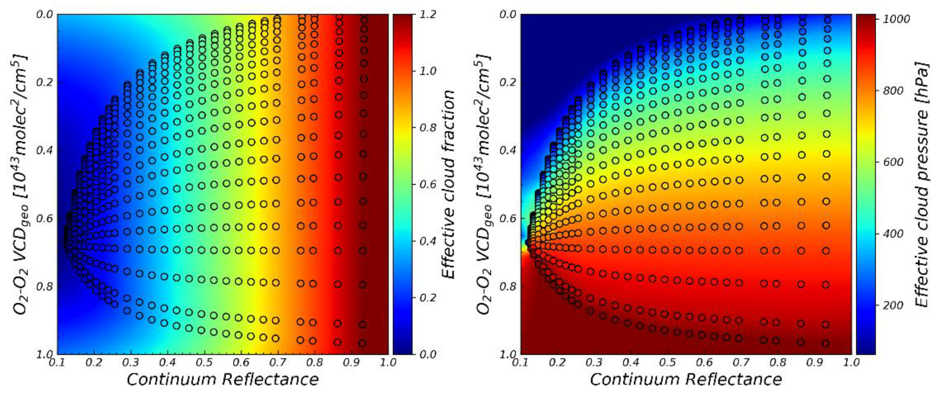
The HECORA algorithm uses measurements of the O₂-O₂ absorption band at 477 nm. This algorithm adopts a LUT similar to the OMCLDO2 algorithm [14,15]. Firstly, we use the VLIDORT [27] instead of the Doubling Adding KNMI [14] model to generate the simulated reflectance spectrum. The VLIDORT model is designed to generate the simultaneous output of the Stokes vector of polarized light and their derivatives for an arbitrary combination of atmospheric and surface properties. VLIDORT can deal with the attenuation of solar and line-of-sight light paths in a pseudo-spherical atmosphere. Secondly, compared with OMCLDO2, we have made some improvements in the DOAS fitting process. OMCLDO2 takes into account the absorption effects of NO₂, O₃, and O₂-O₂ in the DOAS process [15]. HECORA considers more gas species, such as water vapor and Ring structure. The last but most important point is that the LUT we created uses VCD_geo as nodes. The VCD_geo represents the molecular distribution characteristics of a single-pixel in the vertical direction. The VCD_geo is better suited as the LUT node for the cloud retrieval. The specific details of the algorithm are described below.

2.1. Look-up Tables

When creating the LUT, a Lambertian cloud model and an independent pixel approximation (IPA) [28,29] were used in VLIDORT to obtain the simulated spectrum. IPA assumes that a spatial pixel (3.5 × 7 km² in the case of TROPOMI) can be divided into several sub-pixels and there is no lateral transport of radiance between sub-pixel boundaries. Therefore, a pixel containing clouds can be divided into cloud-covered and cloud-free subpixels. The reflectance of top-of-atmosphere (TOA) can be expressed as:

$$R(\lambda ;\theta ,{\theta }_0,\phi ,c,P_c,A_s,P_s){=cR}_{cloud}{(}_{}\lambda ;\theta ,{\theta }_0,\phi {,A}_c,P_s)+(1-c)R_{clear}(\lambda ;\theta ,{\theta }_0,\phi ,A_s,P_s)$$

(1)

where $R(\lambda ;\theta ,{\theta }_0,\phi ,c,P_c,A_s,P_s)$ is the reflectance at TOA for wavelength λ; θ₀ is the solar zenith angle (SZA); θ is the viewing zenith angle (VZA); φ is the relative azimuth angle (RAA); c is the effective cloud fraction; P_c is the cloud top pressure; A_c is the cloud albedo; A_s is the surface albedo (SA); P_s is the surface pressure (SP); R_clear is the reflectance of the clear part of the pixel, and R_cloud is the reflectance of the cloudy part of the pixel. In the simulation process, a Lambertian cloud model with an albedo of 0.8 was selected following the findings of previous studies [2,14,19] proving this to be an adequate choice for cloud correction and trace gas retrieval. The input parameters used for generating the reflectance LUT include SZA, VZA, RAA, SP, SA, effective cloud fraction, and effective cloud pressure. The reflectance from the VLIDORT can be defined as:

$$R=\pi I/(E_0\cos {\theta }_0)$$

(2)

where I is the reflected radiance and E₀ is the corresponding solar irradiance.

Fitting the LUT reflectance spectra by the DOAS technique [30], the continuum reflectance and the O₂-O₂ slant column density (SCD) are calculated. The air-mass factor (AMF) is the ratio of SCD to the VCD of the absorber as viewed by the satellite in the measured radiance spectrum. The AMF value depends on elements such as the vertical distribution of trace gases absorbing in the atmosphere, the length of the optical path, and the reflectivity of the earth’s surface. The length of the light path depends also on the position of the sun and satellite [14]. In the absence of atmospheric scattering, the AMF depends only on geometrical parameters describing the incident solar illumination and the satellite observing geometry. This geometrical AMF, AMF_geo, is expressed as follows:

$$AM{F}_{geo}=1/\cos {\theta }_0+1/\cos \theta$$

(3)

Although HECORA radiative transfer (RT) simulations take into account atmospheric scattering, they use the geometrical VCD, VCD_geo, defined as:

$$VC{D}_{geo}= N_s/AM{F}_{geo}$$

(4)

where $N_s$ is the O₂-O₂ SCD, as nodes for the reflectance LUT instead of using directly the SCD as derived by the DOAS fit. The justification of this choice is to reduce the distance between the O₂-O₂ column nodes in the LUT by normalizing $N_s$ with the AMF_geo and, in this way, decrease the interpolation error in VCD-dimension of the multidimensional space. Just to recap, for fixed values of geometry, SA and SP, we can obtain the continuum reflectance and O₂-O₂ VCD_geo as a function of the effective cloud fraction and cloud pressure as follows:

• Input: $(\theta ,{\theta }_0,\phi ,c,P_c,A_s,P_s)$→ reflectance LUT (Equation (1)) → Output: $R(\lambda ;\theta ,{\theta }_0,\phi {,c,P}_c{,A}_s{,P}_s)$.
• Input: $R(\lambda ;\theta ,{\theta }_0,\phi ,c,P_c,A_s,P_s)$→ DOAS fit → Output: $N_s(\theta ,{\theta }_0,\phi ,c,P_c,A_s,P_s)$; $R_c(\theta ,{\theta }_0,\phi ,c,P_c,A_s,P_s)$, where $R_c$ is the continuum reflectance.
• Input: $N_s(\theta ,{\theta }_0,\phi ,c,P_c,A_s,P_s)$→ Equation (4) → Output: $VC{D}_{geo}(\theta ,{\theta }_0,\phi ,c,P_c,A_s,P_s)$.
• All three steps together form the forward LUT: $(\theta ,{\theta }_0,\phi ,c,P_c,A_s,P_s)$→ LUT_forward→ $(R_c,VC{D}_{geo})$.
  The final objective is to obtain ($c,P_c$) as a function of ($R_c,VC{D}_{geo}$) and the rest of the geometric and surface parameters. Exchanging the ($c,P_c$) and the ($R_c,VC{D}_{geo}$) columns in the input and the output of LUT_forward, we obtain the desired relationship:
• Inverse LUT: ($\theta ,{\theta }_0,\phi ,A_s,P_s,R_c,VC{D}_{geo}$) → LUT_inverse → ($c,P_c$).
  However, there is still a problem to solve. As defined above, the LUT_forward is regular in the input parameters $(\theta ,{\theta }_0,\phi ,c,P_c,A_s,P_s)$ but the output values are scattered in the 2D ($R_c,VC{D}_{geo}$) plan. Accordingly, LUT_inverse has two dimensions ($R_c,VC{D}_{geo}$) where the nodes are not distributed in a regular grid. In order to define the LUT in a multidimensional (7-dimensional) mesh, the input nodes have to be interpolated. We interpolated the LUT_inverse multidimensional scattered data using radial basis functions (RBF) (refer to Veefkind et al., 2016 [15]) leading to the desired inverse LUT in a regular 7-dimensional mesh:
• Inv_regular LUT: LUT_inverse ($\theta ,{\theta }_0,\phi ,A_s,P_s,R_c,VC{D}_{geo}$) → RBF → LUT_{inv_regular} ($\theta ,{\theta }_0,\phi ,A_s,P_s,R_c,VC{D}_{geo}$).

A typical slice of effective cloud fraction and effective cloud pressure is illustrated in Figure 1. The comparison between the HECORA O₂-O₂ VCD_geo nodes and the OMCLDO2 using O₂-O₂ SCD nodes is shown in

Table 1. Comparison of Hefei EMI cloud retrieval algorithm (HECORA) and OMCLDO2 column destinies nodes.

Parameters	Nodes
O2-O2 SCD (OMCLDO2) [${10}^{44}{\mathrm{molec}}^2{\mathrm{cm}}^{-5}$]	0, 0.05, 0.10, 0.15, 0.20, 0.25, 0.30, 0.35, 0.40, 0.45, 0.50, 0.55, 0.60, 0.65, 0.70, 0.75, 0.80, 0.85, 0.90, 0.95, 1.00, 1.10, 1.20
O2-O2 VCDgeo (HECORA) [${10}^{43}{\mathrm{molec}}^2{\mathrm{cm}}^{-5}$]	0, 0.10, 0.20, 0.30, 0.40, 0.50, 0.60, 0.70, 0.80, 0.90, 1.00, 1.10, 1.20, 1.30, 1.40, 1.50, 1.60, 1.70, 1.80, 1.90, 2.00, 2.20, 2.40

. HECORA uses the same number of column density nodes as OMCLDO2; the value of HECORA O₂-O₂ VCD_geo node is 1/5 of the corresponding OMCLDO2 O₂-O₂ SCD node.

2.2. Retrieval Algorithm

HECORA is based on the DOAS method [30,31,32]. By means of a DOAS fit, the O₂-O₂ SCD and reflectance polynomial coefficients are retrieved from the observed reflectance spectrum within the fit window of 460–490 nm. The DOAS equation used in HECORA can be expressed as follows:

$$-InR(\lambda )={\gamma }_0+{\gamma }_1\lambda {+N}_s{\sigma }_{O_2{-O}_2}(\lambda ){+N}_s{}_{{,O}_3}{\sigma }_{O_3}(\lambda ){+N}_{{s,NO}_2}{\sigma }_{{NO}_2}(\lambda )$$

(5)

where R(λ) is the reflectance spectrum, $R_c={\gamma }_0+{\gamma }_1\lambda$ is the continuum reflectance at the wavelength, and λ, $N_s$, $N_s{}_{{,O}_3}$, $N_{{s,NO}_2}$ are the SCD of O₂-O₂, O₃, and NO₂. ${\sigma }_{O_2{-O}_2}$, ${\sigma }_{O_3}$, ${\sigma }_{{NO}_2}$ are the cross-section of O₂-O₂, O₃, and NO₂. The software QDOAS [33] is used to fit the satellite measured reflectance spectrum, using the absorption cross sections and polynomial order as defined in

Table 2. The parameters settings of QDOAS.

Parameters	Resources	Fitting Window/nm
		460–490 nm (O2-O2)
NO2	Vandaele et al. (1998) [34] 240 K	X
O3	Brion et al. (1998) [35] 228 K, 243 K	X
O2-O2	Thalman et al. (2013) [36] 293 K	X
Ring	Chance et al. (1997) [37]	X
Polynomial order		1

. The fitting band is 460–490 nm, the retrieved gas cross-section includes O₂-O₂, O₃, NO₂, H₂O, Ring structure, and the polynomial order is the 1st order. Through DOAS fitting, the continuum reflectance and the O₂-O₂ SCD are calculated.

To calculate the O₂-O₂ VCD_geo and to retrieve cloud parameters, auxiliary data specifying the surface and geometric properties including the SZA, VZA, RAA, SP, and SA are needed. SZA, VZA, solar azimuth angle (SAA), and viewing azimuth angle (VAA) can be obtained from the illumination and viewing geometry information of the specified satellite load, and the RAA can be calculated from SAA and VAA. SP and SA are generated by interpolation from the surface height dataset [38] and surface albedo dataset [39] as a function of latitude and longitude. The effective cloud fraction and cloud pressure are obtained by multidimensional linear interpolation of the above parameters according to the LUT_{inv_regular}.

3. Simulation and Validation of HECORA

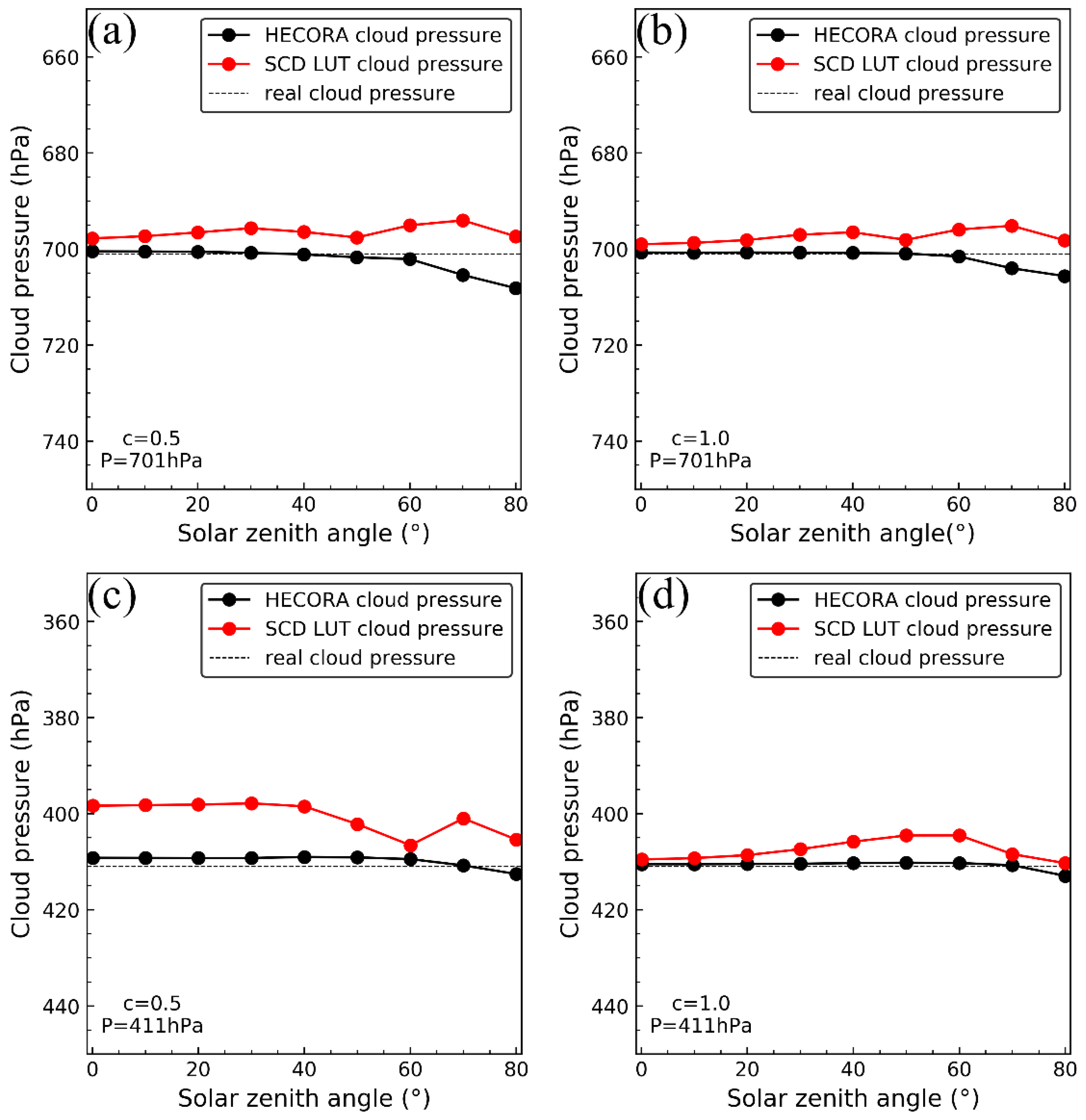
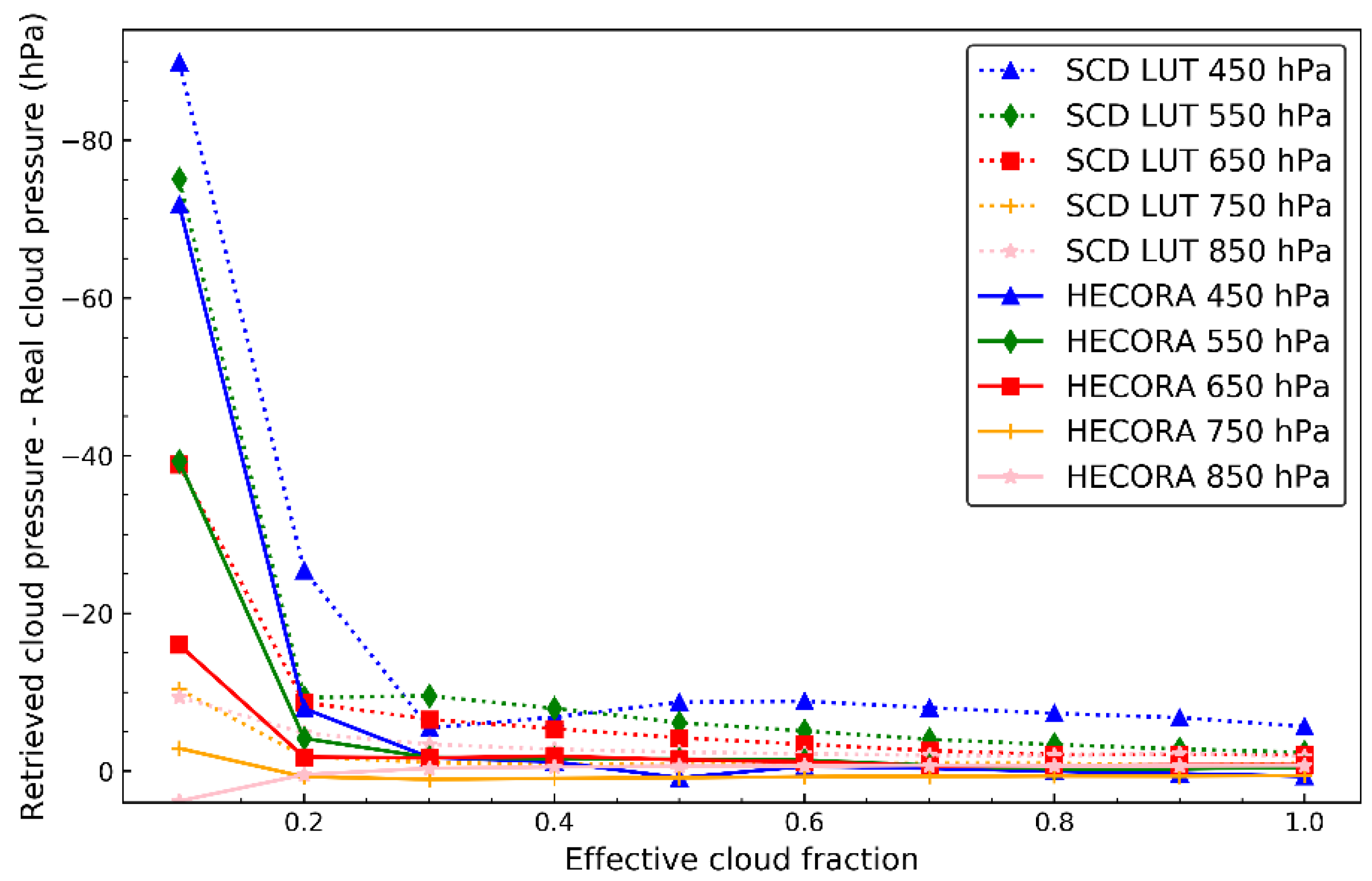
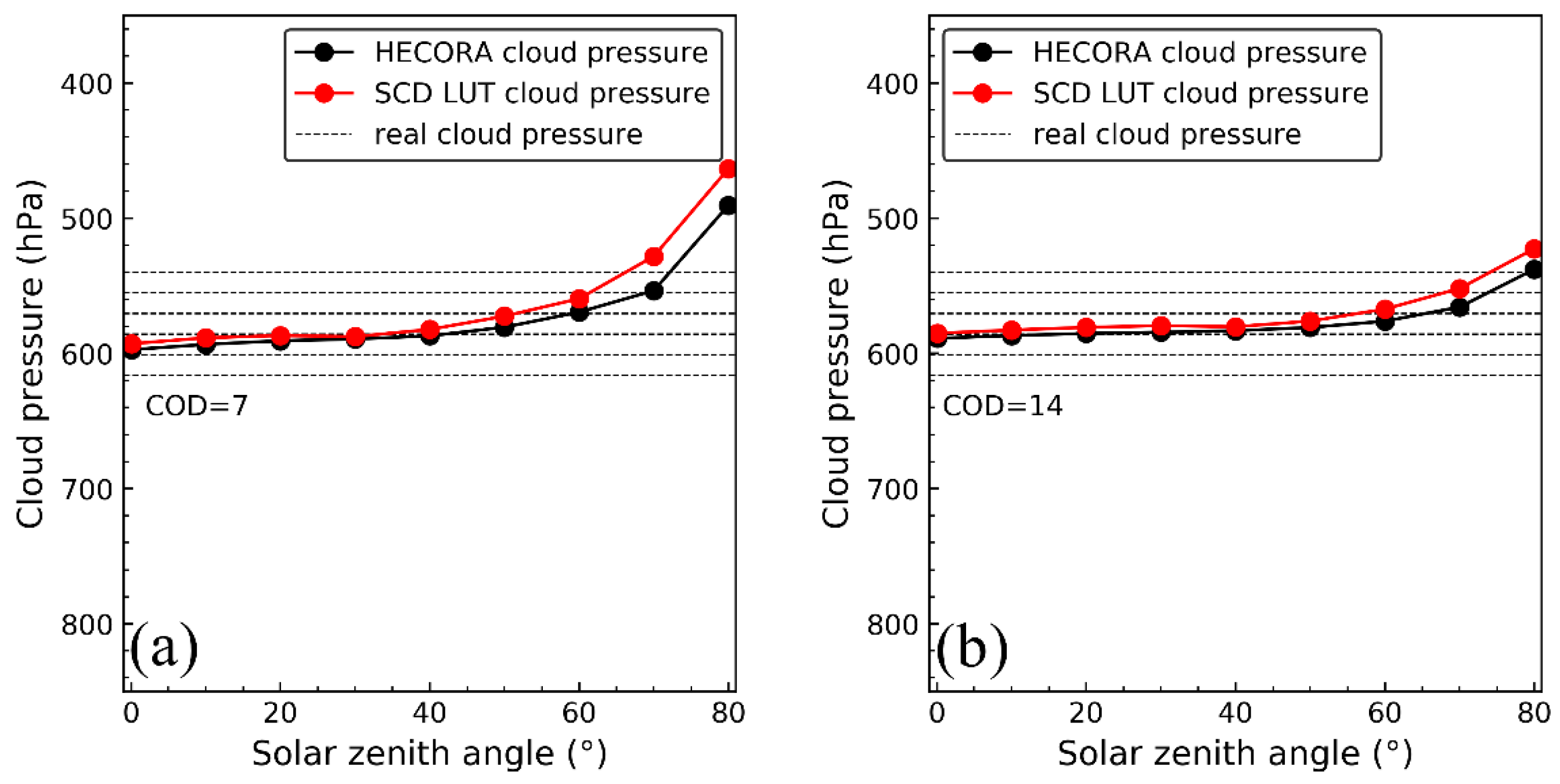
3.1. HECORA Results from the Simulated Spectrum

To verify the HECORA algorithm, the reflectance spectrum was simulated using the VLIDORT radiative transfer model. The simulations are performed on Lambertian cloud and scattering cloud models. To test the accuracy of the HECORA retrieved effective cloud pressure, we created an O₂-O₂ SCD LUT using the same SCD nodes with OMCLDO2 for comparison.

First, we consider the Lambertian cloud. In this model, the cloud is regarded as a Lambertian surface with cloud albedo of 0.8 and ignores transmission. In the simulation, the cloud is at 3 and 7 km, and the corresponding cloud pressure is 701 and 411 hPa. The cloud fraction is set to 0.5 and 1. For all situations, VZA is 0.1 degrees, RAA is 0 degrees, the surface albedo is 0.05, the surface pressure is 1013 hPa, and SZA is 0, 10, 20, 30, 40, 50, 60, 70, and 80 degrees. Figure 2 shows the results of HECORA retrieved cloud pressure as a function of SZA.

In general, the LUT_{inv_regular} used by HECORA performs better than O₂-O₂ SCD LUT. The HECORA retrieval results are very close to the real cloud pressure when SZA is small. When SZA is larger than 60 degrees, HECORA has an overestimation of cloud pressure. However, the O₂-O₂ SCD LUT retrieval results have an underestimation of cloud pressure and the bias is larger than HECORA. When the cloud fraction is 0.5, the average HECORA retrieved cloud pressure is 702.32 hPa, 1.2 hPa higher than the real cloud pressure with a standard deviation of 2.5 hPa. When the cloud fraction is 1.0, the retrieved cloud pressure means is 701.76 hPa, 0.76 hPa higher than the real cloud pressure with a standard deviation of 1.7 hPa. From the retrieved results, when the cloud fraction decreases, the bias between retrieved cloud pressure and real cloud pressure increase. Figure 2c,d also shows the same result, verifying the point of Acarreta [14] that retrieval biases of cloud pressure increase with the decrease of cloud fraction.

To study the stability of HECORA under different cloud fraction conditions, VLIDORT is used to simulate the reflectance of cloud at different pressures (450, 550, 650, 750, 850 hPa) with different cloud fractions and use HECORA to retrieve the cloud pressure. The HECORA retrieved cloud pressure and comparison with the O₂-O₂ SCD LUT retrieval results are presented in Figure 3. When the effective cloud fraction is 1.0, the maximum bias between HECORA retrieved cloud pressure and real cloud pressure is 1.4 hPa, but when the effective cloud fraction is 0.1, the retrieval bias gets worse, the maximum bias is 40.4 hPa. HECORA still shows a more stable performance and has a low bias under different cloud fractions than the O₂-O₂ SCD LUT retrieval results. For clouds of different heights, the bias between both HECORA and O₂-O₂ SCD LUT retrieved cloud pressure increases with the decrease of the cloud fraction. When the cloud fraction is small (≤0.2), the retrieval bias of high cloud is larger than for the low cloud, which proves that the cloud algorithm based on the O₂-O₂ 477 nm absorption bands is less sensitive to the high cloud [15].

By replacing the Lambertian cloud model with the scattering cloud model in VLIDORT, the settings for SZA, VZA, RAA, surface pressure, and surface albedo are the same as for the Lambertian cloud model. The cloud type is set as the water cloud with a droplet size of 0.20 µm. The Ångström exponent is set as 2.0455. The effective radius is set as 10.0 µm. The single scattering albedo is set to 1.00. The refractive index is calculated by Hale and Quarry [40]. The cloud fraction is set to 0.5, and the cloud height is set to 4–5 km (540–617 hPa), with the cloud optical depth (COD) being 7 and 14, respectively. Figure 4 shows the retrieval results, when the COD is 7, the average retrieved cloud pressure from HECORA is 586.81 hPa. While the COD is 14, the average retrieved cloud pressure is 583.62 hPa. The HECORA retrieved cloud pressure is close to the mid-cloud pressure. In contrast to the SCD LUT results, HECORA has a smaller standard deviation. For larger cloud optical thicknesses, the corresponding effective cloud fraction is larger, whereas cloud pressure retrieval errors are smaller.

Overall, HECORA shows a more stable performance than the SCD LUT algorithm both using the Lambertian cloud model and scattering cloud model. In the HECORA algorithm, SZA and VZA are the parameters for calculating VCD_geo. This reduces some of the errors introduced by SZA and VZA by participating directly in the multivariate linear interpolation. On the other hand, HECORA LUT_{inv_regular} column density nodes are denser than those of the OMCLDO2 O₂-O₂ SCD LUT, which reduces the interpolation error generated in the cloud parameter calculation.

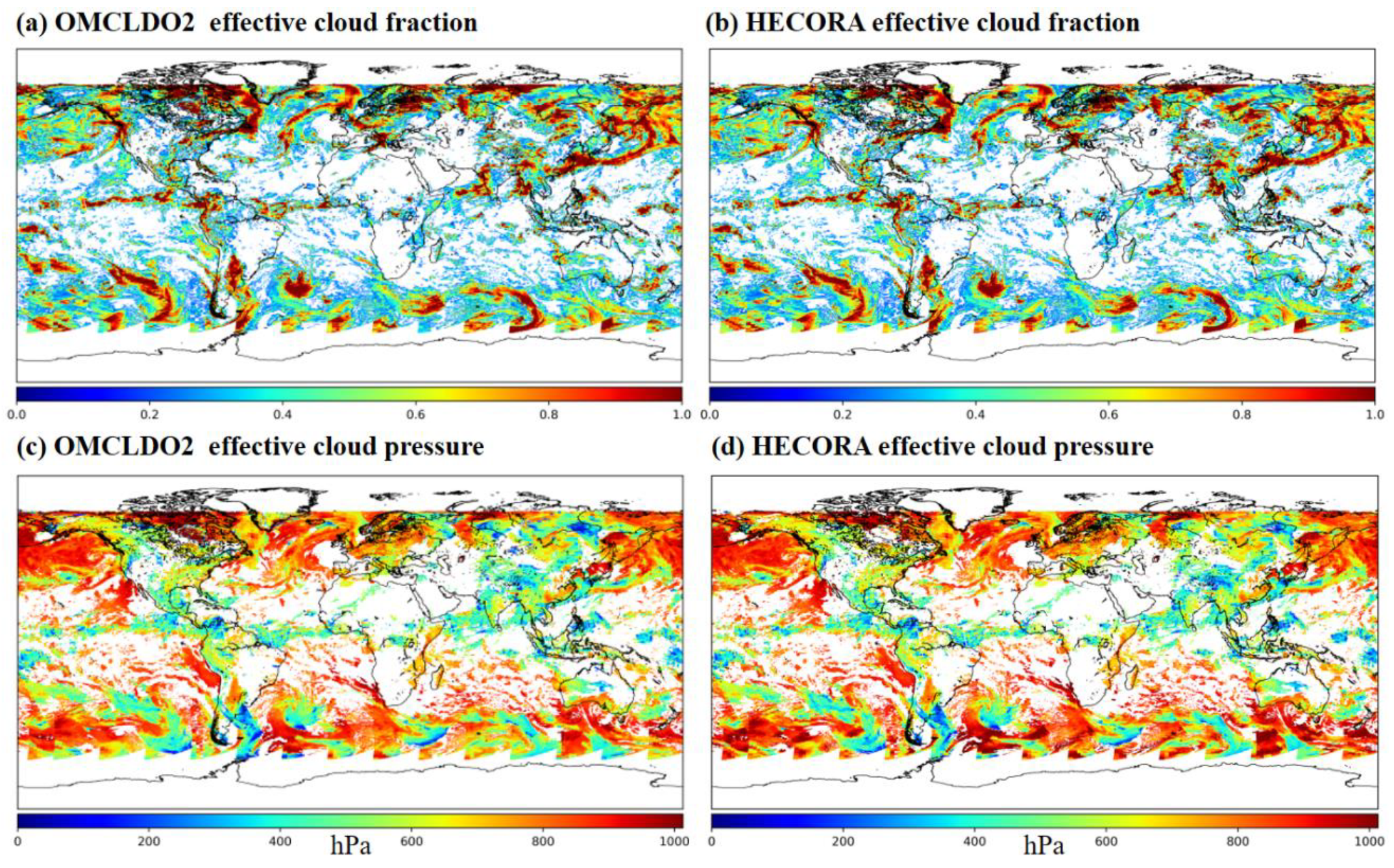
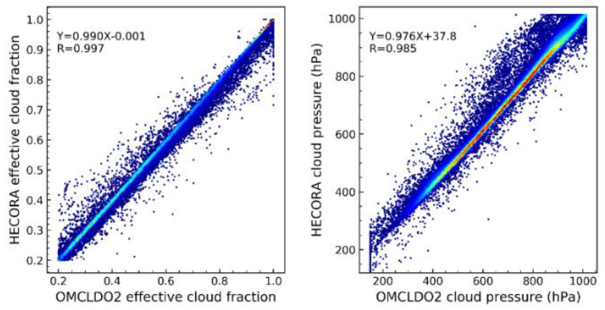
3.2. HECORA Cloud Retrievals from OMI Data

We have applied HECORA to OMI. We selected a random day to compare the global cloud parameters retrieved by HECORA and OMCLDO2 on 1 June 2006. Figure 5 shows the cloud fraction and cloud pressure global spatial distribution. The spatial distribution of effective cloud fraction and effective cloud pressure of OMCLDO2 and HECORA have a strong positive correlation. Figure 6 compares the cloud retrieval results of the OMI orbit 9993 from OMCLDO2 and HECORA on 1 June 2006. From the regression analysis, it is clear that both the retrieval of effective cloud fraction and cloud pressure correlate very well. For the effective cloud fraction, the correlation coefficient is 0.997; for cloud pressure, the correlation coefficient is 0.985. In the case of low cloud pressure, the cloud pressure bias of OMCLDO2 and HECORA increases because of the low sensitivity of the O₂-O₂ 477 nm absorption band to the high cloud. From the comparisons with the OMCLDO2 product, we can conclude that the HECORA can provide reliable results and could be used for cloud retrieval in the hyperspectral load to provide cloud correction for trace gas retrieval.

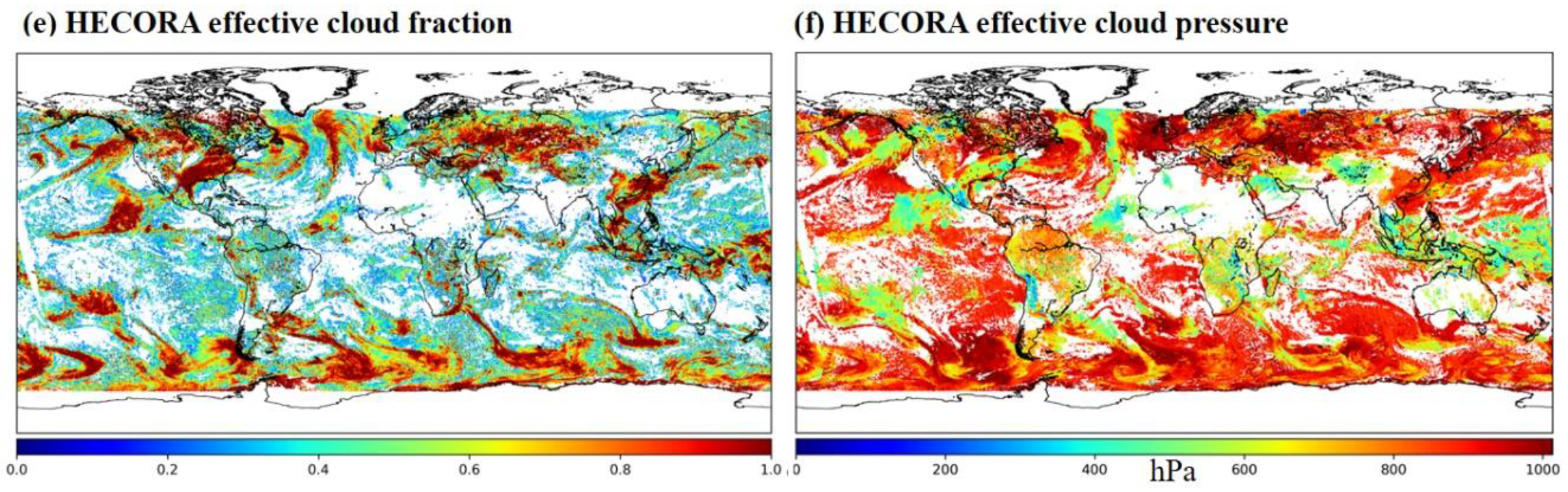
3.3. HECORA Cloud Retrievals from TROPOMI Data

In this section, we compare the cloud parameters retrieved by HECORA and other TROPOMI cloud products and CALIOP. Figure 7 shows the cloud parameters global spatial distribution of TROPOMI from FRESCO+ [20], OCRA/ROCINN [3], and HECORA on 2 January 2019. Since OCRA does not use the assumption that the cloud albedo is 0.8 and cloud albedo is one of the result parameters of ROCINN [3], for a more reasonable comparison with HECORA, the recalculated OCRA cloud fraction was obtained using the following formula:

$$OCRA\_RCF=CF\_crb\times CA\_crb/0.8$$

(6)

In the formula, OCRA_RCF is the recalculated OCRA cloud fraction to compare with HECORA and FRESCO+. CF_crb is the cloud fraction retrieved by OCRA using the CRB (Cloud as Reflecting Boundary) forward model. CA_crb is the cloud albedo used in OCRA.

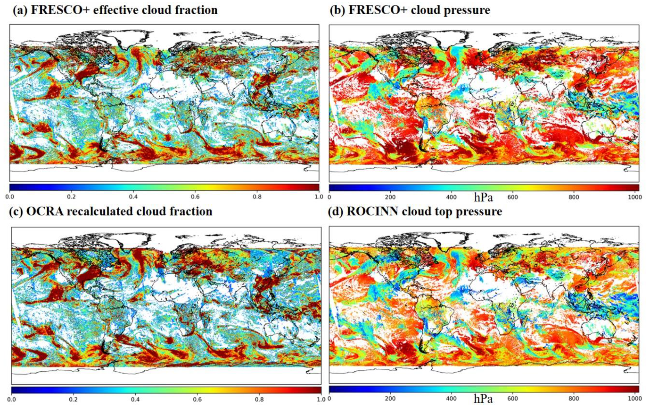
3.3.1. Comparison with Other TROPOMI Cloud Products

We selected the TROPOMI spectrum on 2 January and 1 June 2019 to test the HECORA performance in different seasons. Compared with other existing TROPOMI cloud algorithms, we found that the HECORA retrieval results are well correlated with FRESCO+ (0.90 < R < 0.99). The HECORA retrieved effective cloud fraction also shows consistency with the recalculated OCRA cloud fraction (0.80 < R < 0.91). Compared with ROCINN cloud top pressure results, HECORA cloud pressure results have roughly the same trend as ROCINN (0.83 < R < 0.93). This shows the commonality of different cloud retrieval algorithms. However, in some cases, the HECORA retrieved cloud pressure is larger than those of FRESCO+ and ROCINN. From the comparison, we found: (1) HECORA cloud pressure retrieval results are more correlated with FRESCO+ and OCRA in winter than in summer. (2) The difference of different cloud retrieval algorithms results are smaller in the ocean than in the land. (3) With increasing cloud pressure, the consistency of cloud fraction retrieval results of different algorithms also increases. Overall, HECORA and other cloud products are showing similar trends. Figure 8 shows two typical orbit correlation figures for different cloud products.

Furthermore, we have also statistically analyzed that the long-term results of HECORA, FRESCO+, and OCRA/ROCINN cloud parameters from 5 November 2018 to 4 December 2018 with latitude range are −70 degrees to 70 degrees, excluding the snow and ice cases. During this period, the cloud parameters were widely distributed and representative.

The mean cloud fraction retrieved by FRESCO+, HECORA, and OCRA for different kinds of surface types is shown in

Table 3. Mean cloud fraction parameter and standard deviations for HECORA, FRESCO+, and OCRA, as well as the mean difference for TROPOMI measurements.

	Number of Cases	Cloud Fraction			Difference
		HECORA	FRESCO+	OCRA	HECORA-FRESCO+	HECORA- OCRA
All cases	281961581	$\begin{array}{l}\overline{c}=0.343,\\ SD=0.310\end{array}$	$\begin{array}{l}\overline{c}=0.370,\\ SD=0.338\end{array}$	$\begin{array}{l}\overline{c}=0.340,\\ SD=0.310\end{array}$	$\begin{array}{l}\overline{\Delta c}=-0.0272,\\ SD=0.060\end{array}$	$\begin{array}{l}\overline{\Delta c}=0.0027,\\ SD=0.107\end{array}$
Ocean	271401746	$\begin{array}{l}\overline{c}=0.338,\\ SD=0.307\end{array}$	$\begin{array}{l}\overline{c}=0.363,\\ SD=0.334\end{array}$	$\begin{array}{l}\overline{c}=0.337,\\ SD=0.307\end{array}$	$\begin{array}{l}\overline{\Delta c}=-0.0250,\\ SD=0.053\end{array}$	$\begin{array}{l}\overline{\Delta c}=0.0099,\\ SD=0.099\end{array}$
Land	4677916	$\begin{array}{l}\overline{c}=0.509,\\ SD=0.369\end{array}$	$\begin{array}{l}\overline{c}=0.575,\\ SD=0.396\end{array}$	$\begin{array}{l}\overline{c}=0.404,\\ SD=0.350\end{array}$	$\begin{array}{l}\overline{\Delta c}=-0.0664,\\ SD=0.175\end{array}$	$\begin{array}{l}\overline{\Delta c}=0.1055,\\ SD=0.251\end{array}$
Vegetation	5881919	$\begin{array}{l}\overline{c}=0.455,\\ SD=0.340\end{array}$	$\begin{array}{l}\overline{c}=0.526,\\ SD=0.355\end{array}$	$\begin{array}{l}\overline{c}=0.446,\\ SD=0.329\end{array}$	$\begin{array}{l}\overline{\Delta c}=-0.0781,\\ SD=0.121\end{array}$	$\begin{array}{l}\overline{\Delta c}=0.0092,\\ SD=0.148\end{array}$

. We can see that the differences of cloud fraction are minimal (~0.03), which is expected as the effective cloud fraction is mainly determined by the reflectance measurements performed in the non-absorbed part of the spectrum. The effective cloud fraction retrieved by HECORA is lower than the one retrieved by FRESCO+ and larger than OCRA_RCF, especially for the land and vegetation cases.

The mean cloud pressure and the pressure difference between FRESCO+, HECORA, and ROCINN are shown in

Table 4. Mean cloud pressure parameter and standard deviations for HECORA, FRESCO+, and ROCINN, as well as the mean difference for TROPOMI measurements.

	Number of Cases	Cloud Pressure (hPa)			Difference (hPa)
		HECORA	FRESCO+	ROCINN	HECORA -FRESCO+	HECORA -ROCINN
All cases	281961581	$\begin{array}{l}\overline{P}=852,\\ SD=163\end{array}$	$\begin{array}{l}\overline{P}=825,\\ SD=207\end{array}$	$\begin{array}{l}\overline{P}=700,\\ SD=163\end{array}$	$\begin{array}{l}\overline{\Delta P}=27.2,\\ SD=122.9\end{array}$	$\begin{array}{l}\overline{\Delta P}=152.0,\\ SD=132.4\end{array}$
Ocean	271401746	$\begin{array}{l}\overline{P}=856,\\ SD=157\end{array}$	$\begin{array}{l}\overline{P}=827,\\ SD=207\end{array}$	$\begin{array}{l}\overline{P}=702,\\ SD=161\end{array}$	$\begin{array}{l}\overline{\Delta P}=29.0,\\ SD=118.22\end{array}$	$\begin{array}{l}\overline{\Delta P}=153.8,\\ SD=127.7\end{array}$
Land	4677916	$\begin{array}{l}\overline{P}=795,\\ SD=212\end{array}$	$\begin{array}{l}\overline{P}=801,\\ SD=209\end{array}$	$\begin{array}{l}\overline{P}=658,\\ SD=192\end{array}$	$\begin{array}{l}\overline{\Delta P}=-5.9,\\ SD=192.6\end{array}$	$\begin{array}{l}\overline{\Delta P}=137.4,\\ SD=208.4\end{array}$
Vegetation	5881919	$\begin{array}{l}\overline{P}=738,\\ SD=223\end{array}$	$\begin{array}{l}\overline{P}=764,\\ SD=211\end{array}$	$\begin{array}{l}\overline{P}=643,\\ SD=198\end{array}$	$\begin{array}{l}\overline{\Delta P}=-25.8,\\ SD=214.4\end{array}$	$\begin{array}{l}\overline{\Delta P}=94.6,\\ SD=195.1\end{array}$

. The mean pressures are 852 ± 163 hPa by HECORA and 825 ± 207 hPa by FRESCO+. ROCINN results show sharply different results. We also analyzed the pressure differences for different surface types. Over the oceans, the HECORA mean effective cloud pressure is greater than that of FRESCO+ and ROCINN. However, over land and vegetation, the effective cloud pressure retrieved by HECORA is lower than FRESCO+, much higher than ROCINN. Over land, the mean cloud pressure of HECORA, FRESCO+, and ROCINN is 795 ± 212 hPa, 801 ± 209 hPa, and 658 ± 192 hPa. The land surface is the surface type with the smallest difference between the results of the three cloud retrieval algorithms. The cloud pressure retrieval results from HECORA are much greater than in ROCINN, which is due to the fact that the visible band used by HECORA is more sensitive to the middle of the cloud, while the ROCINN results using the O₂ A-band are closer to the actual cloud top pressure [15], the O₂ A-band and O₂-O₂ band have different absorption and scattering characteristics, and its sensitivity to the cloud and surface is different.

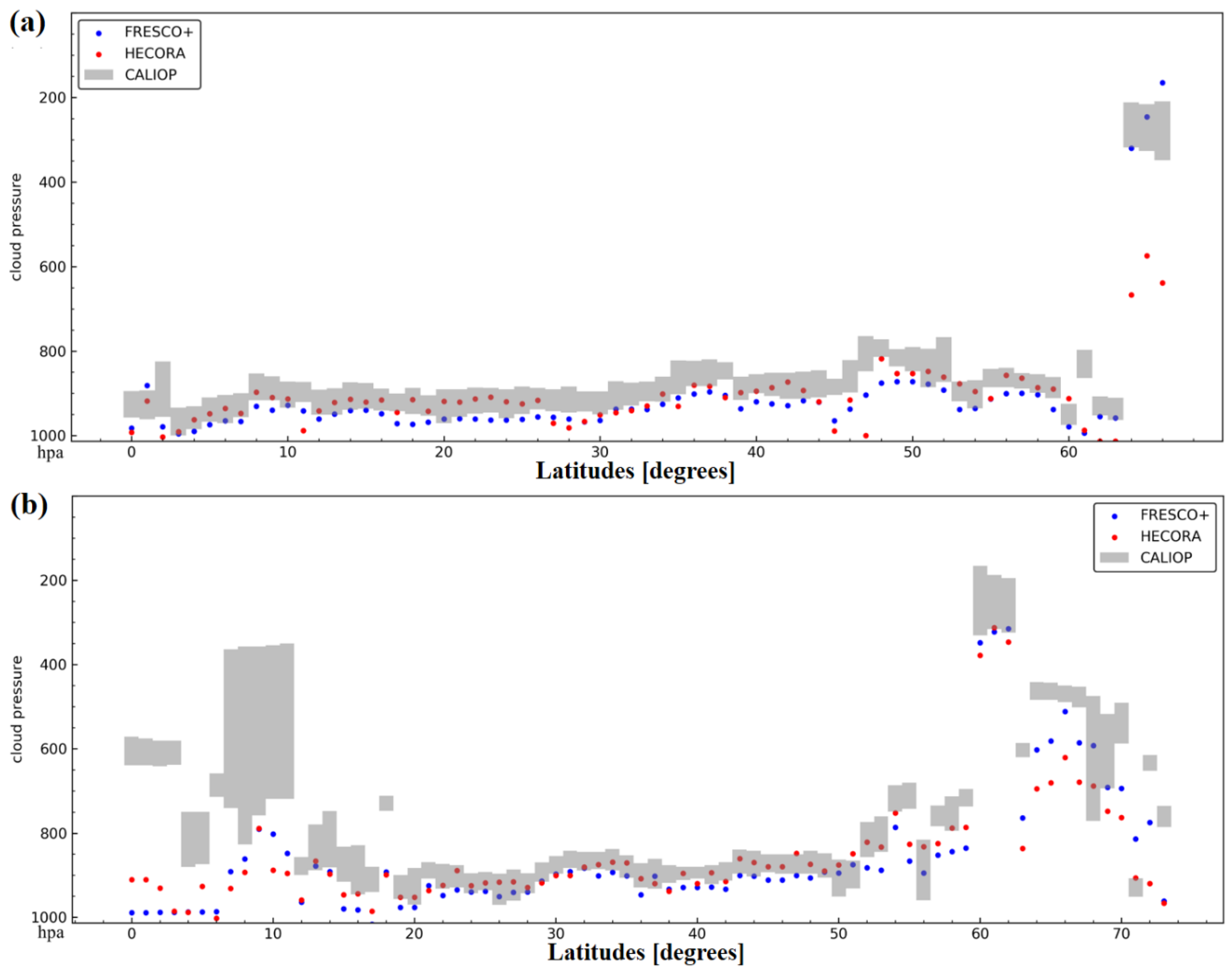
3.3.2. Comparison with CALIOP

The primary payload aboard CALIPSO is CALIOP. CALIOP is an elastic backscatter lidar that transmits linearly polarized laser light at 532 and 1064 nm. It measures range-resolved backscatter intensities at both wavelengths using a three-channel receiver, which mainly provides cloud and aerosol information. In this study, we choose the CALIOP 2 Level product Cloud Layer with version 3.4. We compared the cloud pressure formation from HECORA and FRESCO+ with the CALIOP cloud layer from 5 November to 4 December 2018. For the one considered monthly data, we further filter as follows:

(1)

CALIOP cloud layer is a single layer; cloud optical depth is greater than 4.

(2)

For every CALIOP pixel, the collocated TROPOMI pixel we selected is within ±0.025 degrees of the CALIOP latitude and longitude.

(3)

HECORA cloud fraction is greater than 0.1.

(4)

A local overpass time difference within ±30 min.

(5)

CALIOP cloud top pressure and cloud base pressure have been successfully retrieved.

Those criteria leave us with 11,230 cases. We take the average of CALIOP cloud top pressure and cloud base pressure as the CALIOP cloud pressure. The mean pressure of CALIOP is 733 ± 218 hPa; this value retrieved by FRESCO+ and HECORA is 823 ± 185 hPa and 843 ± 142 hPa, respectively. That means that the cloud pressure retrieved by FRESCO+ and HECORA is greater than CALIOP, but the FRESCO+ retrieval result is closer to CALIOP. Then, classifying all cases into oceans, land, and vegetation based on MODIS NDVI products, the comparison results are shown in

Table 5. Mean cloud pressure and standard deviations for HECORA and FRESCO+ of TROPOMI, as well as CALIOP.

	Number of Cases	Cloud Pressure (hPa)
		HECORA	FRESCO+	CALIOP
All cases	11,230	$\overline{P}=843,SD=142$	$\overline{P}=823,SD=185$	$\overline{P}=733,SD=218$
Ocean	10,810	$\overline{P}=845,SD=143$	$\overline{P}=826,SD=184$	$\overline{P}=738,SD=218$
Land	203	$\overline{P}=850,SD=157$	$\overline{P}=793,SD=191$	$\overline{P}=696,SD=213$
Vegetation	217	$\overline{P}=800,SD=169$	$\overline{P}=752,SD=199$	$\overline{P}=684,SD=234$

. For different surface types, the average values of FRESCO+ are closer to the CALIOP cloud layer pressure than those retrieved by HECORA.

We have also compared the global distribution of cloud pressure retrieved by HECORA and FRESCO+ for TROPOMI measurements and consider the CALIOP results as true cloud pressure. The comparison results of two typical CALIOP orbits are shown in Figure 9. For the selected orbit on 6 and 28 November 2018, HECORA retrieval results are closer to the CALIOP cloud pressure in low cloud conditions, whereas FRESCO+ performs better in high and thick clouds. The comparison results are consistent with Acarreta’s [14] view that the O₂-O₂ distribution in the atmosphere has a lower profile shape than O₂, increasing the sensitivity to lower clouds in principle.

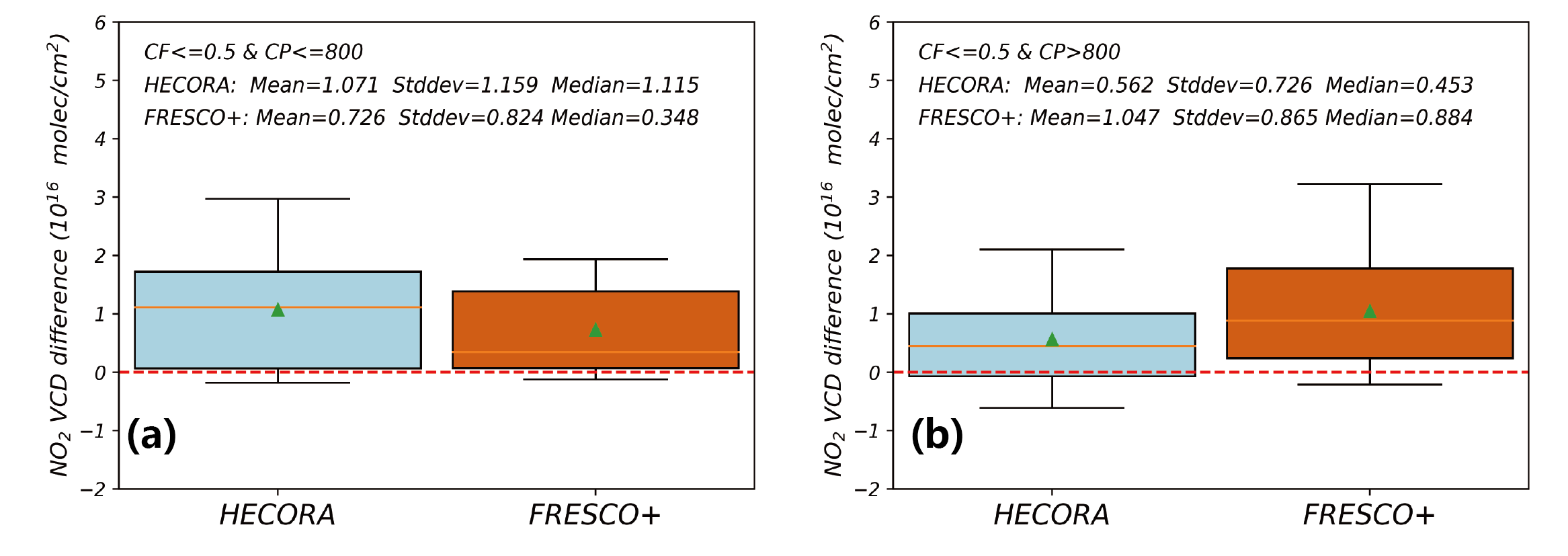
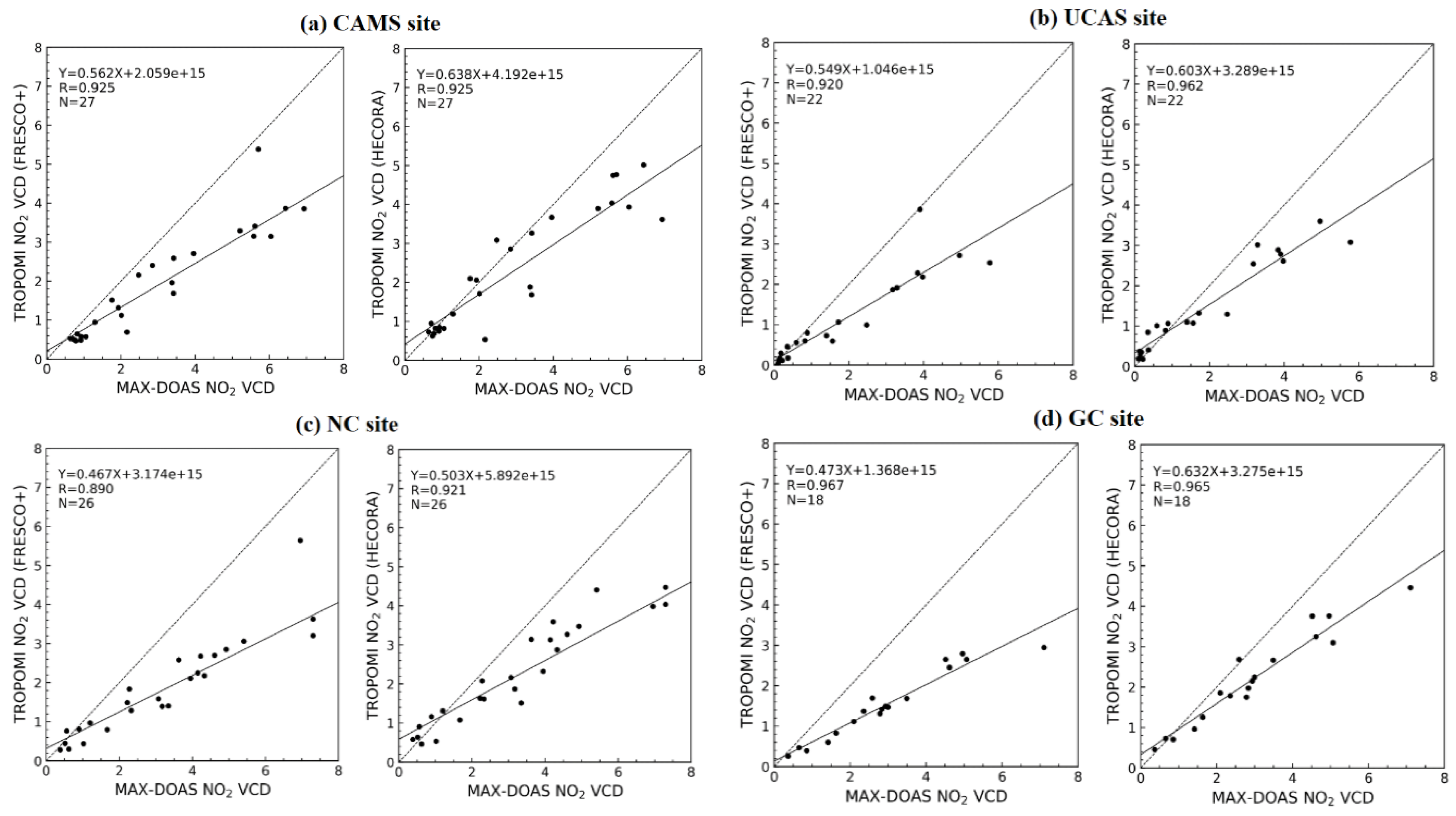
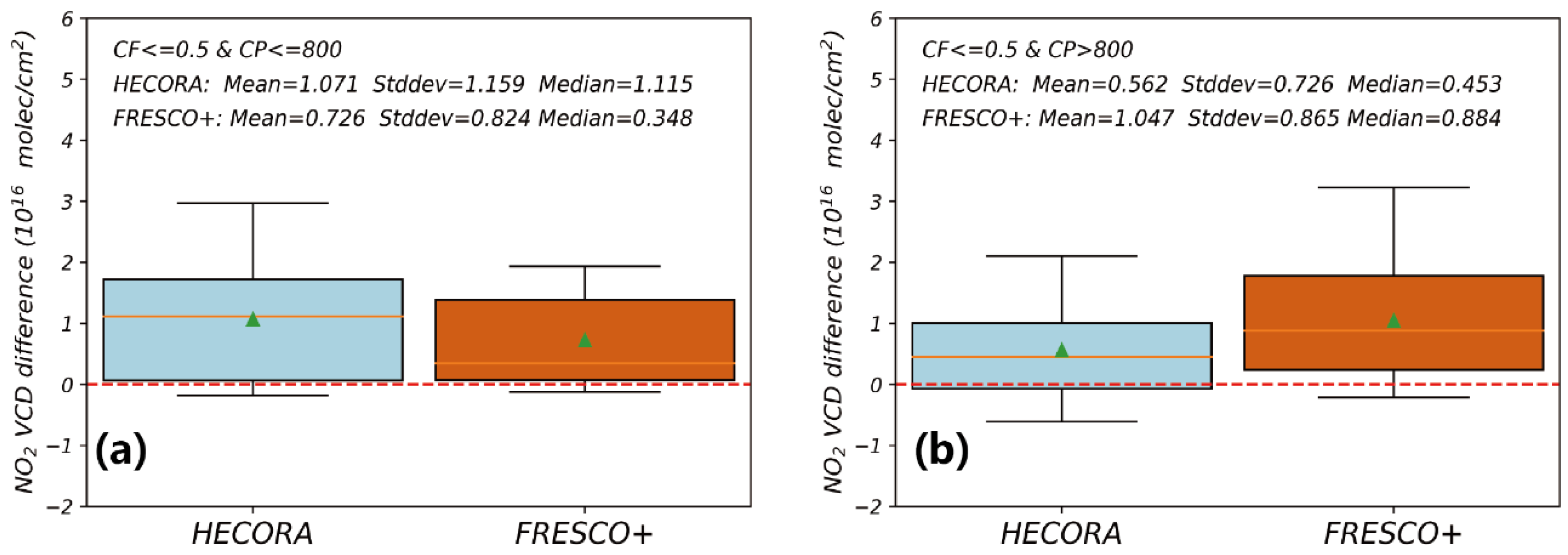
3.3.3. Application to TROPOMI NO₂ Retrieval and Comparison with MAX-DOAS

The TROPOMI NO₂ operational retrieval algorithm uses FRESCO+ to correct cloud effects [41]. The purpose of developing HECORA is to correct cloud effects in the retrieval of trace gases from the EMI of China. However, the current EMI spectral calibration work is still in progress, so we use TROPOMI spectra to test the effect of HECORA in correcting NO₂ retrieval results. The NO₂ VCD retrieval algorithm used here is previously implemented for the EMI NO₂ operation product (refer to Zhang et al., 2019 [42]), and has been adapted to the TROPOMI instrument. The NO₂ retrieval method in general followed three steps: (1) NO₂ SCDs fitting in the wavelength range of 405–465 nm by using the DOAS technique. (2) Stratospheric and tropospheric NO₂ AMF were calculated pixel-by-pixel by the VLIDORT model, using daily high-resolution NO₂ a priori profile from the WRF-Chem model. (3) A modified reference sector method [43] is used to estimate the stratospheric contribution from the total column and derive the final tropospheric NO₂ VCD. During the AMFs calculation, auxiliary information including cloud fraction and cloud top pressure are needed in the second step. The FRESCO+ cloud parameters involved in the calculation are the cloud pressure, the cloud fraction, and the cloud radiance fraction from the NO₂ spectra window itself at 440 nm.

To explore the effect of cloud parameters on the tropospheric NO₂ retrieval, we compared the ground-based multiaxial differential optical absorption spectroscopy (MAX-DOAS) observation data with TROPOMI NO₂ VCD to evaluate the performance of HECORA and FRESCO+. The multiaxial differential optical absorption spectroscopy (MAX-DOAS) is used to measure concentrations of trace gases from the ground. MAX-DOAS can retrieve aerosol profiles with the corresponding aerosol properties (e.g., AOD) and trace gas profiles using the measured spectrum information. Four observation sites in the Chinese Academy of Meteorological Sciences (CAMS, 39.9472° N, 116.3206° E), University of Chinese Academy of Sciences (UCAS, 40.408° N, 116.675° E), Nancheng (NC, 39.781° N, 116.127° E), Gucheng (GC, 39.149° N, 115.734° E) are selected. The analyzed variable is the average value of tropospheric NO₂ VCD between 13:00 and 14:00 every day from 5 November to 17 December 2018. These four observation sites are located in the Beijing-Tianjin-Hebei region of China, where air pollution is relatively serious. The choice of time period fully considers the possible impact of different cloud parameters on tropospheric NO₂ VCD. For every TROPOMI pixel collocated with a MAX-DOAS site, the TROPOMI longitude and latitude are the value of MAX-DOAS ± 0.1° (~10 km). The average value of NO₂ VCD that meets the above conditions is the corresponding TROPOMI results.

The TROPOMI NO₂ retrieval results with effective cloud fraction smaller than 0.5 using two algorithms are compared with the MAX-DOAS measurements. The MAX-DOAS retrieval algorithm used in this paper can be found in Xing et al. (2017) [44]. Figure 10a–d shows tropospheric NO₂ VCD using two cloud retrieval algorithms and the MAX-DOAS NO₂ VCD from CAMS, UCAS, NC, and GC at four observation sites. The correlations between tropospheric NO₂ VCD using two cloud retrieval algorithms and MAX-DOAS NO₂ VCD at four sites are very high, especially for UCAS and GC, and GC and UCAS sites have a relatively lower NO₂ VCD than the other two sites. Results show that both cloud retrieval algorithms are effective in correcting the effect of cloud on the tropospheric NO₂ VCD retrieval.

Based on the comparison in Section 3.3.2, we found that under low altitude cloud conditions, the cloud pressure retrieved by HECORA is closer to that of the CALIOP cloud layer products than FRESCO+. For polluted areas, NO₂ is mainly concentrated in the boundary layer, usually less than 2 km (>800 hPa). The small difference of cloud pressure input will make a meaningful impact on the retrieval results of the NO₂ concentration on low altitude cloud pixels [20]. Figure 11 shows the difference between the observed values of MAX-DOAS and TROPOMI using HECORA and FRESCO+ for cloud correction under different cloud pressure ranges. We choose 800 hPa as the boundary between high and low clouds. As can be seen in Figure 11, whether using HECORA or FRESCO+ for cloud correction, the TROPOMI NO₂ retrieval results tend to be smaller than the MAX-DOAS observations, especially in such polluted areas. The underestimation part is related to the large satellite pixels. The average effect of the satellite pixels is unable to capture the spatial gradient of NO₂ [45]. Under low cloud conditions, the mean, median, and standard deviation of the differences between the TROPOMI retrieval results using HECORA cloud parameters and MAX-DOAS observations are smaller. This shows that the cloud correction effect of HECORA under low cloud conditions is stronger than that of FRESCO+. In contrast, TROPOMI NO₂ products using FRESCO+ perform well when the cloud pressure is smaller than 800 hPa. In summary, HECORA and FRESCO+ have their own advantages. HECORA is suitable for low cloud pixels, especially for polluting pixels with high NO₂ concentrations. FRESCO+ is suitable for cloud correction of high cloud pixels. Considering the current situation of air pollution in China, it is appropriate to use HECORA cloud parameters for cloud correction in the EMI trace gas retrieval.

4. Conclusions

We have developed a new cloud retrieval algorithm called HECORA based on the O₂-O₂ 477 nm absorption band. Compared to the OMCLDO2 algorithm, the main updates include (1) adopting a new radiative transfer model VLIDORT, (2) improving DOAS retrieval settings, and (3) the first use of O₂-O₂ VCD nodes to retrieve cloud information. We use an O₂-O₂ VCD_geo LUT with denser column density nodes to retrieve cloud parameters. HECORA is intended to improve the accuracy of cloud information retrieved from hyperspectral satellite loads and planned to be applied to EMI.

We first verify HECORA using the VLIDORT simulated spectrum. When the Lambertian cloud model is used in the simulation, the results of HECORA cloud pressure are mostly consistent with those of VLIDORT, and the error is small (<20 hPa); the retrieval error decreases with the increase of cloud fraction. When the scattering cloud model is used in the simulation, the cloud pressure retrieval results are close to the middle cloud pressure. For both cloud models, HECORA’s retrieval results are better than those using the O₂-O₂ SCD LUT. The SCD LUT uses the same SCD nodes as the OMCLDO2 algorithm.

The validation of HECORA was also carried out by comparisons of the retrieved effective cloud fraction and cloud pressure with the OMI OMCLDO2, TROPOMI FRESCO+, OCRA/ROCINN, and CALIOP cloud layer products. For OMI measurements, comparisons showed a very good agreement between HECORA and OMCLDO2. Applying HECORA to TROPOMI, the HECORA cloud fraction retrieval results have a high correlation coefficient with the FRESCO+ results and the recalculated OCRA cloud fraction; the cloud pressure retrieval results from different algorithms have some differences. To compare the performance of HECORA and FRESCO+ at different cloud heights, we compared the cloud pressure from HECORA and FRESCO+ with the CALIOP cloud layer product. In the low cloud conditions, the HECORA performs better, while the FRESCO+ retrieval results are slightly better in the high cloud conditions. These differences have a significant impact on the retrieval results of NO₂.

Finally, the HECORA and FRESCO+ cloud parameters were used for the retrieval of TROPOMI NO₂ VCD and compared with the MAX-DOAS observations in the same region. The retrieval results of TROPOMI tropospheric NO₂ VCD are in good agreement with those of MAX-DOAS. The cloud correction effect of HECORA under low cloud conditions is greater than that of FRESCO+. Combined with the vertical distribution of NO₂ in typical pollution areas, HECORA is suitable for cloud correction for trace gas retrieval in China, and is expected to be applied to EMI shortly thereafter.

5. Discussion

We found a common phenomenon that FRESCO+ and HECORA overestimate the cloud pressure of high clouds in some cases. The possible reasons are as follows. When the cloud is very high (<400 hPa), the cloud type is mainly ice clouds. The optical properties of ice clouds are complicated by the geometries of the ice particles, the uncertainties in ice crystal concentration, and their size spectra [46]. The cloud model used by two cloud algorithms set cloud parameters more like water clouds. The scattering and absorption characteristics of ice clouds and water clouds are quite different. This makes HECORA and FRESCO+ unable to correctly retrieve the cloud pressure of very high clouds.

Although HECORA applied the O₂-O₂ VCD_geo LUT to cloud retrieval algorithms for the first time, it has achieved good performance. However, there are still some aspects of HECORA that need to be improved in future work. For example, HECORA performs worse than FRESCO+ in high cloud conditions. HECORA does not account for the change of the absorption cross-section of the O₂-O₂ molecule with temperature. The IPA assumption used by HECORA does not consider any anisotropic parameters, such as the anisotropic surface BRDF. We will consider these ideas to improve HECORA as an orientation in the next release of HECORA. Finally, we will be applying HECORA to EMI as soon as possible.

References

1. King, M.D.; Platnick, S.; Menzel, W.P.; Ackerman, S.A.; Hubanks, P.A. Spatial and temporal distribution of clouds observed by MODIS onboard the Terra and Aqua satellites. IEEE Trans. Geosci. Remote Sens. 2013, 51, 3826–3852. [Google Scholar] [CrossRef]
2. Stammes, P.; Sneep, M.; de Haan, J.F.; Veefkind, J.P.; Wang, P.; Levelt, P.F. Effective cloud fractions from the Ozone Monitoring Instrument: Theoretical framework and validation. J. Geophys. Res. 2008, 113. [Google Scholar] [CrossRef] [Green Version]
3. Loyola, D.G.; Gimeno García, S.; Lutz, R.; Argyrouli, A.; Romahn, F.; Spurr, R.J.; Pedergnana, M.; Doicu, A.; Molina García, V.; Schüssler, O. The operational cloud retrieval algorithms from TROPOMI on board Sentinel-5 Precursor. Atmos. Meas. Tech. 2018, 11, 409–427. [Google Scholar] [CrossRef] [Green Version]
4. Liu, X.; Newchurch, M.; Loughman, R.; Bhartia, P. Errors resulting from assuming opaque Lambertian clouds in TOMS ozone retrieval. J. Quant. Spectrosc. Radiat. Transf. 2004, 85, 337–365. [Google Scholar] [CrossRef]
5. Kokhanovsky, A.; Rozanov, V. The uncertainties of satellite DOAS total ozone retrieval for a cloudy sky. Atmos. Res. 2008, 87, 27–36. [Google Scholar] [CrossRef]
6. Wagner, T.; Beirle, S.; Deutschmann, T.; Grzegorski, M.; Platt, U. Dependence of cloud properties derived from spectrally resolved visible satellite observations on surface temperature. Atmos. Chem. Phys. 2008, 8, 2299–2312. [Google Scholar] [CrossRef] [Green Version]
7. Levelt, P.F.; van den Oord, G.H.J.; Dobber, M.R.; Malkki, A.; Huib, V.; Johan de, V.; Stammes, P.; Lundell, J.O.V.; Saari, H. The ozone monitoring instrument. IEEE Trans. Geosci. Remote Sens. 2006, 44, 1093–1101. [Google Scholar] [CrossRef]
8. Callies, J.; Corpaccioli, E.; Eisinger, M.; Hahne, A.; Lefebvre, A. GOME-2-Metop’s second-generation sensor for operational ozone monitoring. ESA Bull. 2000, 102, 28–36. [Google Scholar]
9. Munro, R.; Lang, R.; Klaes, D.; Poli, G.; Retscher, C.; Lindstrot, R.; Huckle, R.; Lacan, A.; Grzegorski, M.; Holdak, A. The GOME-2 instrument on the Metop series of satellites: Instrument design, calibration, and level 1 data processing-an overview. Atmos. Meas. Tech. 2016, 9, 1279–1301. [Google Scholar] [CrossRef] [Green Version]
10. Veefkind, J.; Aben, I.; McMullan, K.; Förster, H.; De Vries, J.; Otter, G.; Claas, J.; Eskes, H.; De Haan, J.; Kleipool, Q. TROPOMI on the ESA Sentinel-5 Precursor: A GMES mission for global observations of the atmospheric composition for climate, air quality and ozone layer applications. Remote Sens. Environ. 2012, 120, 70–83. [Google Scholar] [CrossRef]
11. Salomonson, V.V.; Barnes, W.; Maymon, P.W.; Montgomery, H.E.; Ostrow, H. MODIS: Advanced facility instrument for studies of the Earth as a system. IEEE Trans. Geosci. Remote Sens. 1989, 27, 145–153. [Google Scholar] [CrossRef]
12. Winker, D.M.; Vaughan, M.A.; Omar, A.; Hu, Y.; Powell, K.A.; Liu, Z.; Hunt, W.H.; Young, S.A. Overview of the CALIPSO mission and CALIOP data processing algorithms. J. Atmos. Ocean. Technol. 2009, 26, 2310–2323. [Google Scholar] [CrossRef]
13. Yin, H.; Sun, Y.; Liu, C.; Zhang, L.; Lu, X.; Wang, W.; Shan, C.; Hu, Q.; Tian, Y.; Zhang, C. FTIR time series of stratospheric NO 2 over Hefei, China, and comparisons with OMI and GEOS-Chem model data. Opt. Express 2019, 27, A1225–A1240. [Google Scholar] [CrossRef] [PubMed]
14. Acarreta, J.; De Haan, J.; Stammes, P. Cloud pressure retrieval using the O2-O2 absorption band at 477 nm. J. Geophys. Res. Atmos. 2004, 109. [Google Scholar] [CrossRef] [Green Version]
15. Veefkind, J.P.; de Haan, J.F.; Sneep, M.; Levelt, P.F. Improvements to the OMI O2–O2 operational cloud algorithm and comparisons with ground-based radar–lidar observations. Atmos. Meas. Tech. 2016, 9, 6035–6049. [Google Scholar] [CrossRef] [Green Version]
16. Koelemeijer, R.; Stammes, P.; Hovenier, J.; De Haan, J. A fast method for retrieval of cloud parameters using oxygen A band measurements from the Global Ozone Monitoring Experiment. J. Geophys. Res. Atmos. 2001, 106, 3475–3490. [Google Scholar] [CrossRef] [Green Version]
17. R, D.G.L.; Thomas, W.; Spurr, R.; Mayer, B. Global patterns in daytime cloud properties derived from GOME backscatter UV-VIS measurements. Int. J. Remote Sens. 2010, 31, 4295–4318. [Google Scholar]
18. Rodriguez, D.G.L.; Thomas, W.; Livschitz, Y.; Ruppert, T.; Albert, P.; Hollmann, R. Cloud Properties Derived From GOME/ERS-2 Backscatter Data for Trace Gas Retrieval. IEEE Trans. Geosci. Remote Sens. 2007, 45, 2747–2758. [Google Scholar] [CrossRef]
19. Wang, P.; Tuinder, O.; Stammes, P. Cloud retrieval algorithm for GOME-2: FRESCO+. Available online: http://www.temis.nl/docs/AD_FRESCO.pdf (accessed on 15 September 2020).
20. Wang, P.; Stammes, P.; Pinardi, G.; Van Roozendael, M. FRESCO+: An improved O 2 A-band cloud retrieval algorithm for tropospheric trace gas retrievals. Atmos. Chem. Phys. 2008, 8, 6565–6576. [Google Scholar] [CrossRef] [Green Version]
21. Platnick, S.; King, M.D.; Ackerman, S.A.; Menzel, W.P.; Baum, B.A.; Riedi, J.C.; Frey, R.A. The MODIS cloud products: Algorithms and examples from terra. IEEE Trans. Geosci. Remote Sens. 2003, 41, 459–473. [Google Scholar] [CrossRef] [Green Version]
22. Kleipool, Q.; Ludewig, A.; Babić, L.; Bartstra, R.; Braak, R.; Dierssen, W.; Dewitte, P.-J.; Kenter, P.; Landzaat, R.; Leloux, J. Pre-launch calibration results of the TROPOMI payload on-board the Sentinel-5 Precursor satellite. Atmos. Meas. Tech. 2018, 11, 6439–6479. [Google Scholar] [CrossRef] [Green Version]
23. Vasilkov, A.; Yang, E.-S.; Marchenko, S.; Qin, W.; Lamsal, L.; Joiner, J.; Krotkov, N.; Haffner, D.; Bhartia, P.K.; Spurr, R. A cloud algorithm based on the O2-O2 477 nm absorption band featuring an advanced spectral fitting method and the use of surface geometry-dependent Lambertian-equivalent reflectivity. Atmos. Meas. Tech. 2018, 11, 4093–4107. [Google Scholar] [CrossRef] [Green Version]
24. Deschamps, P.; Fouquart, Y.; Tanré, D.; Herman, M.; Lenoble, J.; Buriez, J.; Dubuisson, P.; Parol, F.; Vanbauce, C.; Grassl, H. Study on the Effects of Scattering on the Monitoring of Atmospheric Constituents. Rep. 3838, ESA Contract No. 9740/91/NL/BI. 1994. Available online: https://scholar.google.com/scholar?lookup=0&q=Study+on+the+effects+of+scattering+on+the+monitoring+of+atmospheric+constituents.+Rep.+3838,+ESA+contract+no.+9740/91/NL/BI%3B+1994.&hl=en&as_sdt=0,5 (accessed on 3 August 2020).
25. Zhang, C.; Liu, C.; Chan, K.L.; Hu, Q.; Liu, H.; Li, B.; Xing, C.; Tan, W.; Zhou, H.; Si, F. First observation of tropospheric nitrogen dioxide from the Environmental Trace Gases Monitoring Instrument onboard the GaoFen-5 satellite. Light Sci. Appl. 2020, 9, 1–9. [Google Scholar] [CrossRef] [PubMed] [Green Version]
26. Zhang, C.; Liu, C.; Wang, Y.; Si, F.; Zhou, H.; Zhao, M.; Su, W.; Zhang, W.; Chan, K.L.; Liu, X. Preflight evaluation of the performance of the Chinese environmental trace gas monitoring instrument (EMI) by spectral analyses of nitrogen dioxide. IEEE Trans. Geosci. Remote Sens. 2018, 56, 3323–3332. [Google Scholar] [CrossRef]
27. Spurr, R.J. VLIDORT: A linearized pseudo-spherical vector discrete ordinate radiative transfer code for forward model and retrieval studies in multilayer multiple scattering media. J. Quant. Spectrosc. Radiat. Transf. 2006, 102, 316–342. [Google Scholar] [CrossRef]
28. Cahalan, R.F.; Ridgway, W.; Wiscombe, W.J.; Bell, T.L.; Snider, J.B. The albedo of fractal stratocumulus clouds. J. Atmos. Sci. 1994, 51, 2434–2455. [Google Scholar] [CrossRef]
29. Zuidema, P.; Evans, K.F. On the validity of the independent pixel approximation for boundary layer clouds observed during ASTEX. J. Geophys. Res. Atmos. 1998, 103, 6059–6074. [Google Scholar] [CrossRef]
30. Plat, U. Differential Optical Absorption Spectroscopy. Air Monitoring by Spectroscopic Techniques; Chemical Analysis Series; John Wiley & Sons: Hoboken, NJ, USA, 1994; Volume 127, pp. 27–84. [Google Scholar]
31. Perner, D.; Ehhalt, D.; Pätz, H.; Platt, U.; Röth, E.; Volz, A. OH-radicals in the lower troposphere. Geophys. Res. Lett. 1976, 3, 466–468. [Google Scholar] [CrossRef]
32. Platt, U.; Perner, D.; Pätz, H. Simultaneous measurement of atmospheric CH2O, O3, and NO2 by differential optical absorption. J. Geophys. Res. Ocean. 1979, 84, 6329–6335. [Google Scholar] [CrossRef]
33. Danckaert, T.; Fayt, C.; Van Roozendael, M.; De Smedt, I.; Letocart, V.; Merlaud, A.; Pinardi, G. QDOAS Software User Manual. 2012. Available online: http://uv-vis.aeronomie.be/software/QDOAS/QDOAS_manual.pdf (accessed on 15 September 2020).
34. Vandaele, A.C.; Hermans, C.; Simon, P.C.; Carleer, M.; Colin, R.; Fally, S.; Merienne, M.-F.; Jenouvrier, A.; Coquart, B. Measurements of the NO2 absorption cross-section from 42,000 cm−1 to 10,000 cm−1 (238–1000 nm) at 220 K and 294 K. J. Quant. Spectrosc. Radiat. Transf. 1998, 59, 171–184. [Google Scholar] [CrossRef] [Green Version]
35. Brion, J.; Chakir, A.; Charbonnier, J.; Daumont, D.; Parisse, C.; Malicet, J. Absorption spectra measurements for the ozone molecule in the 350–830 nm region. J. Atmos. Chem. 1998, 30, 291–299. [Google Scholar] [CrossRef]
36. Thalman, R.; Volkamer, R. Temperature dependent absorption cross-sections of O 2–O 2 collision pairs between 340 and 630 nm and at atmospherically relevant pressure. Phys. Chem. Chem. Phys. 2013, 15, 15371–15381. [Google Scholar] [CrossRef] [PubMed]
37. Chance, K.V.; Spurr, R.J. Ring effect studies: Rayleigh scattering, including molecular parameters for rotational Raman scattering, and the Fraunhofer spectrum. Appl. Opt. 1997, 36, 5224–5230. [Google Scholar] [CrossRef] [PubMed] [Green Version]
38. Danielson, J.J.; Gesch, D.B. Global Multi-Resolution Terrain Elevation Data 2010 (GMTED2010); US Department of the Interior, US Geological Survey: SanDiego, CA, USA, 2011.
39. Tilstra, L.; Tuinder, O.; Wang, P.; Stammes, P. Surface reflectivity climatologies from UV to NIR determined from Earth observations by GOME-2 and SCIAMACHY. J. Geophys. Res. Atmos. 2017, 122, 4084–4111. [Google Scholar] [CrossRef]
40. Hale, G.M.; Querry, M.R. Optical constants of water in the 200-nm to 200-μm wavelength region. Appl. Opt. 1973, 12, 555–563. [Google Scholar] [CrossRef]
41. Van Geffen, J.; Boersma, K.; Eskes, H.; Maasakkers, J.; Veefkind, J. TROPOMI ATBD of the Total and Tropospheric NO2 Data Products; DLR Document. 2014. Available online: https://sentinel.esa.int/documents/247904/2476257/Sentinel-5P-TROPOMI-ATBD-NO2-data-products (accessed on 15 September 2020).
42. Zhang, C.; Liu, C.; Hu, Q.; Cai, Z.; Su, W.; Xia, C.; Zhu, Y.; Wang, S.; Liu, J. Satellite UV-Vis spectroscopy: Implications for air quality trends and their driving forces in China during 2005–2017. Light Sci. Appl. 2019, 8, 100. [Google Scholar] [CrossRef] [Green Version]
43. Beirle, S.; Hörmann, C.; Jöckel, P.; Liu, S.; Penning de Vries, M.; Pozzer, A.; Sihler, H.; Valks, P.; Wagner, T. The STRatospheric Estimation Algorithm from Mainz (STREAM): Estimating stratospheric NO2 from nadir-viewing satellites by weighted convolution. Atmos. Meas. Tech. (AMT) 2016, 9, 2753–2779. [Google Scholar] [CrossRef] [Green Version]
44. Xing, C.; Liu, C.; Wang, S.; Chan, K.; Gao, Y.; Huang, X.; Su, W.; Zhang, C.; Dong, Y.; Fan, G. Observations of the summertime atmospheric pollutants vertical distributions and the corresponding ozone production in Shanghai, China. Atmos. Chem. Phys. Discuss 2017, 2017, 1–31. [Google Scholar] [CrossRef] [Green Version]
45. Chan, K.L.; Wiegner, M.; van Geffen, J.; De Smedt, I.; Alberti, C.; Cheng, Z.; Ye, S.; Wenig, M. MAX-DOAS measurements of tropospheric NO2 and HCHO in Munich and the comparison to OMI and TROPOMI satellite observations. Atmos. Meas. Tech. 2020, 13, 4499–4520. [Google Scholar] [CrossRef]
46. Cotton, W.R.; Bryan, G.; Van den Heever, S.C. Storm and Cloud Dynamics; Academic Press: Salt Lake City, UT, USA, 2010. [Google Scholar]
Figure 1. The slice of effective cloud fraction (left panel) and effective cloud pressure (right panel) for solar zenith angle of 32.9°,viewing zenith angle of 32.9°, relative azimuth angle of 0°, surface pressure of 1013 hPa, surface albedo of 0.075. The background colors show the cloud parameter values under the look-up tables (LUT) from interpolation and extrapolation. The different circles represent the nodes of different O2-O2 vertical column densities (VCDgeo) and continuum reflectance (Rc) distributions, and only a part of the nodes are displayed.
Remotesensing 12 03039 g001
Figure 2. Results of retrieved cloud pressure with different effective cloud fraction and effective cloud pressure under the vector linearized discrete ordinate radiative transfer (VLIDORT) simulated spectrum: (a) Results of retrieved effective cloud pressure (c = 0.5, Pc = 701 hPa), (b) results of retrieved effective cloud pressure (c = 1.0, Pc = 701 hPa), (c) results of retrieved effective cloud pressure (c = 0.5, Pc = 411 hPa), (d) results of retrieved effective cloud pressure (c = 1.0, Pc = 411 hPa).
Remotesensing 12 03039 g002
Figure 3. The bias between retrieved effective cloud pressure and the VLIDORT simulated cloud pressure with different effective cloud fractions. The surface pressure (SP) is fixed at 1013 hPa, the solar zenith angle (SZA) is 30 degrees, the viewing zenith angle (VZA) is 0.1 degrees, the relative azimuth angle (RAA) is 0 degrees, and the surface albedo (SA) is 0.05.
Remotesensing 12 03039 g003
Figure 4. Results of retrieved effective cloud pressure with different effective cloud fractions using the scattering cloud model. (a) Results of retrieved effective cloud pressure (COD = 7); (b) results of retrieved effective cloud pressure (COD = 14).
Remotesensing 12 03039 g004
Figure 5. Cloud retrieval results from OMCLDO2 and HECORA for the ozone monitoring instrument (OMI) on 1 June 2006. (a) OMCLDO2 effective cloud fraction, (b) HECORA effective cloud fraction, (c) OMCLDO2 effective cloud pressure, (d) HECORA effective cloud pressure.
Remotesensing 12 03039 g005
Figure 6. Comparison of cloud retrieval results from OMCLDO2 and HECORA for OMI orbit 9993.
Remotesensing 12 03039 g006
Figure 7. Results of cloud parameters from HECORA, the fast retrieval scheme for clouds from the oxygen A-band (FRESCO+), and optical cloud recognition algorithm/retrieval of cloud information using neural networks (OCRA/ROCINN) for the tropospheric monitoring instrument (TROPOMI) global spatial distribution in 2 January 2019. (a) FRESCO+ effective cloud fraction, (b) FRESCO+ cloud pressure, (c) OCRA recalculated cloud fraction, (d) ROCINN cloud top pressure, (e) HECORA effective cloud fraction, (f) HECORA effective cloud pressure.
Remotesensing 12 03039 g007aRemotesensing 12 03039 g007b
Figure 8. Comparison results of cloud retrieval from different cloud products. (a) TROPOMI orbit 6331 (2 January 2019), (b) TROPOMI orbit 8451 (1 June 2019).
Remotesensing 12 03039 g008
Figure 9. Vertical distribution of cloud pressure of TROPOMI HECORA, FRESCO+, and CALIOP. (a) The selected orbit on 6 November 2018, (b) the selected orbit on 28 November 2018.
Remotesensing 12 03039 g009
Figure 10. TROPOMI NO2 VCD using FRESCO+ and HECORA compared with the multiaxial differential optical absorption spectroscopy (MAX-DOAS). (a) Results in the Chinese Academy of Meteorological Sciences (CAMS) site, (b) results in the University of Chinese Academy of Sciences (UCAS) site, (c) results in the Nancheng (NC) site, (d) results in the Gucheng (GC) site. The solid line is the corresponding linear fitting line. The dashed line is a reference line.
Remotesensing 12 03039 g010
Figure 11. Tropospheric NO2 VCD difference between TROPOMI and MAX-DOAS under different cloud pressure ranges. The vertical axis represents the observed value of MAX-DOAS minus TROPOMI. The red dashed lines indicate zero values, the green triangle represents the average of the differences. The maximum, minimum, median, and upper and lower quartiles are shown in the boxplot and some outliers are filtered out. (a) Retrieved cloud fraction (CF) ≤ 0.5 and retrieved cloud pressure (CP) ≤ 800 hPa, (b) CF ≤ 0.5 and CP > 800 hPa.
Remotesensing 12 03039 g011