A Fast and Effective Method for Unsupervised Segmentation Evaluation of Remote Sensing Images

Abstract

The segmentation of remote sensing images with high spatial resolution is important and fundamental in geographic object-based image analysis (GEOBIA), so evaluating segmentation results without prior knowledge is an essential part in segmentation algorithms comparison, segmentation parameters selection, and optimization. In this study, we proposed a fast and effective unsupervised evaluation (UE) method using the area-weighted variance (WV) as intra-segment homogeneity and the difference to neighbor pixels (DTNP) as inter-segment heterogeneity. Then these two measures were combined into a fast-global score (FGS) to evaluate the segmentation. The effectiveness of DTNP and FGS was demonstrated by visual interpretation as qualitative analysis and supervised evaluation (SE) as quantitative analysis. For this experiment, the ‘‘Multi-resolution Segmentation’’ algorithm in eCognition was adopted in the segmentation and four typical study areas of GF-2 images were used as test data. The effectiveness analysis of DTNP shows that it can keep stability and remain sensitive to both over-segmentation and under-segmentation compared to two existing inter-segment heterogeneity measures. The effectiveness and computational cost analysis of FGS compared with two existing UE methods revealed that FGS can effectively evaluate segmentation results with the lowest computational cost.

1. Introduction

With the rapid development of remote sensing technology, high spatial resolution remote sensing images can be more easily obtained and widely used in a variety of applications [1,2,3,4]. Compared with the low- and medium-resolution remote sensing image, the high-resolution remote sensing image contains more detailed spatial information, but the spectral resolution is lower [5]. If the pixel-based analysis method which only uses the spectral information of the image is applied to the high-resolution image, its rich spatial information will be ignored and more noise will be produced [6,7]. Therefore, geographic object-based image analysis (GEOBIA) has begun to emerge and can achieve better accuracy in the high-resolution image [8,9,10].

The purpose of GEOBIA is to effectively utilize the spatial and texture information of high-resolution images [11,12]. The first step of GEOBIA is to segment the image into a series of meaningful objects. Therefore, the segmentation effect has an important impact on the subsequent feature extraction, classification, etc. [13]. A large number of segmentation algorithms have been applied in GEOBIA. For example, the deep learning method [14,15], multi-resolution segmentation [16], watershed segmentation [17,18], and hybrid segmentation [19,20] are widely used in GEOBIA. In most of the segmentation algorithms, there is a parameter called “scale” to control the size of the object, which greatly affects the final segmentation results and the effect of GEOBIA [21,22,23,24]. Hence, evaluating image segmentation is critical to select optimal scale and obtain better segmentation results for subsequent analysis.

Direct evaluation methods can be classified into three variants: analytical evaluation (AE), supervised evaluation (SE), and unsupervised evaluation (UE) [25]. AE determinates the optimal scales by comparing a series of segmentation results by human visual inspection and it is widely used for simplicity [26]. However, it is time-consuming and greatly influenced by human subjectivity. SE evaluates segmentation quantitatively using discrepancy criteria between the segmentation results and the reference segmentation result [11,27,28]. SE overcomes human error and produces a more reliable, objective, and quantitative evaluation. Therefore, SE needs to build a reference dataset manually. However, building the whole reference dataset for high-resolution remote sensing image is tedious and time-consuming and involves some subjectivity. Moreover, the computation process and the matching algorithm between objects are very complex. The above disadvantages make it difficult to be applied in specific practical applications. UE needs no reference segmentation result and measures segmentation quality by defining evaluation criteria, which is based on human interpretation of the ideal segmentation result [24,29,30,31,32]. In the absence of prior knowledge of segmented images, UE can objectively evaluate the segmentation results without being affected by human subjectivity. UE can not only be used to evaluate the segmentation results but also be used for the selection of the segmentation algorithm and the setting of the segmentation parameters. Furthermore, since no prior knowledge is required, it is also used for segmentation parameters optimization which is not available in other segmentation evaluation methods [29,33,34]. Therefore, compared with AE and SE, UE is more applicable and more practical.

The widely accepted ideal state of segmentation results is as follows: for the features that can express the characteristics of objects, the objects should be consistent and homogeneous; the adjacent objects should have significant heterogeneity [35]. In the UE, the homogeneity goodness index is used to measure the homogeneity within the objects, and the heterogeneity goodness index is used to measure the heterogeneity between the objects, and then the two indexes are combined to evaluate the segmentation quality. There are texture-based and spectrum-based methods for homogeneity [36,37]. However, because computing the spectral information is simple and most of the segmentation methods are based on the spectral information, the research of the goodness based on the spectral information is far greater than the goodness based on the texture information. Compared with homogeneity, only spectrum-based methods are available for heterogeneity.

The area-weighted variance (WV) and global Moran’s I (MI) are often used to compute the homogeneity within objects and the heterogeneity between objects, respectively [29,30,38,39]. Higher WV values indicate the higher dispersion of spectral values and the lower homogeneity within the object. Higher MI values indicate the higher the correlation and the lower the heterogeneity between objects. Wang et al. [22] proposed a UE method using WV and Jeffries–Matusita (JM) distance to evaluate segmentation quality. JM computes the spectral separability distance between objects to measure the spectral heterogeneity. Wang et al. [24] used between-segment heterogeneity (BSH) instead of MI to compute the heterogeneity between objects. The main difference between BSH and MI is that BSH uses the local statistics of the target object and its adjacent objects, while MI uses the global statistics of the whole image. The spectral value of a pixel can be represented as a vector, so Yang et al. [31] used the spectral angle to measure the spectral homogeneity between objects. Although the existing methods play a certain role in the quality evaluation of image segmentation, most of the heterogeneity evaluation methods need to compute the differences between adjacent objects. In other words, we need to construct the region adjacency graph (RAG) to get the adjacency between objects. However, the process of RAG construction is very complex and time-consuming, especially when the image size is large and the segmentation scale value is low. As the size of the image increases, the number of segmented objects is increasing, and the construction time of RAG is also increasing geometrically, which makes the existing methods difficult to apply in practice. Up to now, far too little attention has been paid to computational cost. Therefore, a fast and effective UE method is needed.

In this paper, we present a fast and effective UE method for remote sensing images using the WV and difference to neighbor pixels (DTNP). Different from most existing heterogeneity evaluation measures, the difference with neighboring pixels was calculated in DTNP which avoids the time-consuming RAG construction and computation with neighboring objects. The WV and DTNP were used to compute the intra-segment homogeneity and inter-segment heterogeneity, respectively. The WV and DTNP were then combined into a fast-global score (FGS) to evaluate segmentation. In order to demonstrate the effectiveness and computational cost of DTNP and FGS, the other two existing methods were compared in the qualitative and quantitative analysis.

The main contributions of this paper are as follows: (1) Most of the existing inter-segment heterogeneity measures are based on RAG to compute the difference with neighboring objects, but the proposed DTNP computes the difference with neighboring pixels and is sensitive to both under-segmentation and over-segmentation. (2) The proposed FGS performs comparable to JM and WM, but the computational cost is much lower than JM and WM, which can be used for optimal segmentation parameter selection and segmentation parameter optimization. (3) Evaluating image segmentation by combining intra-segment homogeneity and inter-segment heterogeneity is more effective than evaluating image segmentation only by inter-segment heterogeneity, indicated by comparison of Section 3.1 and Section 3.2

The rest of this paper is arranged as follows. In Section 2, we elaborate on the specific details of the proposed method as well as the experimental areas and data. Section 3 gives the experimental results. Section 4 and Section 5 describe the discussion and conclusions, respectively.

2. Materials and Methods

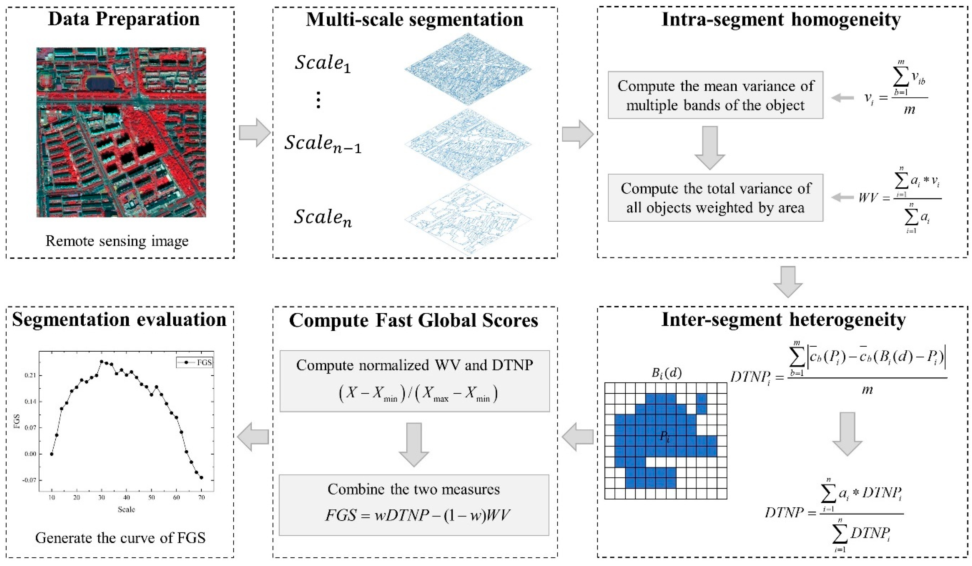
2.1. Overview

The schematic of segmentation evaluation through FGS which combines WV and DTNP is shown in Figure 1. The FGS was computed by the intra-segment homogeneity and the inter-segment heterogeneity under a series of different segmentation scales. First, we represented intra-segment homogeneity by computing the WV. Second, we represented inter-segment heterogeneity by computing the DTNP. Third, WV and DTNP were combined into FGS, and the curve of FGS with scale was generated for segmentation evaluation. Note that the WV and DTNP were computed in eCognition Developer 9.0 [40], FGS was computed in Python 3.6, equipped in a computer with 64-bit Windows 10, Intel Core i5-8265U CPU at 1.8 GHz, and 8 GB RAM. The algorithm has been open source (https://github.com/mfzhao1998/FGS).

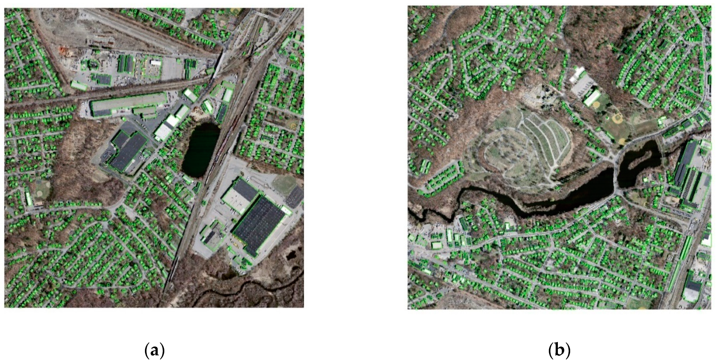
2.2. Study Area and Data

A Gaofen-2 (GF-2) scene in Tongzhou District, Beijing, China, which was acquired on 9 September 2018, was applied to evaluate the performance of the proposed method. The GF-2 images contain four multi-spectral bands (blue, green, red, and near-infrared) with a resolution of 3.2 m and a panchromatic band with a resolution of 0.8 m. The NNDiffuse Pan Sharpening [41] which performs best when the combination of all multispectral bands covers the spectral range of the panchromatic raster in ENVI software [42] was used to fuse panchromatic data with multispectral data to obtain multispectral data with a resolution of 0.8 m. Four subsets of a residential area, an industrial area, a farmland area, and a mixed area in the GF-2 scene were selected for testing the proposed method (Figure 2).

2.3. Image Segmentation

Image segmentation is a technique that segments the image into different image regions with high homogeneity and mutual connection, corresponding to the objects or spatial structure features of interest. The ‘‘Multi-resolution Segmentation’’ algorithm in eCognition Developer 9.0 was used to perform image segmentation. The details of the algorithm can refer to Benz et al. [43]. The algorithm starts from a single pixel and uses the “bottom-up” region merging method to form polygon objects with different sizes (scales). Two adjacent image regions merge and grow. The judgment of merging depends on the heterogeneity of adjacent objects. Several small objects can be merged into a large object through several steps. The merging of two objects must ensure that the heterogeneity of them is less than the given threshold. The final object size is decided by this threshold. Therefore, this threshold can be regarded as a scale parameter. Other segmentation parameters include color factor and shape factor, and the weights between them. The color factor is the spectral characteristics of the image—the weight of each band. The shape factor is composed of two parameters, smoothness and compactness, which can prevent the image object from being broken too much, so that the segmented object has the shape characteristics of the actual object.

In this paper, the color factor to shape factor ratio was set to 9:1. All spectral bands were used and given the same weight. Smoothness and compactness were given the same weight. A series of segmentation produced by the Multi-resolution Segmentation was carried out with different scale parameters at intervals of 2, ranging from 10 to 70, so as to adapt to different scenes such as cities and suburbs.

2.4. Unsupervised Evaluation Using Fast-Global Score

Most evaluation methods mainly consider intra-segment homogeneity and inter-segment heterogeneity, excluding internal continuity and boundary complexity that are difficult to apply to remote sensing images [25,30]. Appropriate segmentation parameters were defined that minimized intra-segment homogeneity and maximized inter-segment heterogeneity [29]. In other words, the difference within an object is the lowest, and the difference between the objects is the highest. First, the variance was used as global intra-segment homogeneity, weighted by each segment’s area. It is defined as follows:

$$v_i=\frac{{{\displaystyle \sum }}_{b=1}^m{v}_{ib}}{m}$$

(1)

where m is the band number of the image, $v_{ib}$ is the variance of object i in band m, and $v_i$ is the mean variance of object i averaged by all bands.

$$WV=\frac{{{\displaystyle \sum }}_{i=1}^n{a}_i\ast v_i}{{{\displaystyle \sum }}_{i=1}^n{a}_i}$$

(2)

where n is the total object number and $a_i$ is the area of object i. $\mathrm{WV}$ gives the same weight to each band, and we give $v_i$ different weight according to the size of the area, avoiding the instability caused by small segments. Third, the DTNP of each object was computed as follows:

$$DTN{P}_i=\frac{{{\displaystyle \sum }}_{b=1}^m\left|{\overline{c}}_b\left(P_i\right)-{\overline{c}}_b\left(B_i\left(d\right)-P_i\right)\right|}{m}$$

(3)

$B_{i\left(d\right)}$ is the extended bounding box of object i with distance d (Figure 3),which is equal to $\left\{\left(\mathrm{x},\mathrm{y}\right):{\mathrm{x}}_{\min }\left(\mathrm{i}\right)-\mathrm{d}\le \mathrm{x}\le {\mathrm{x}}_{\max }\left(\mathrm{i}\right)+\mathrm{d},{\mathrm{y}}_{\min }\left(\mathrm{i}\right)-\mathrm{d}\le \mathrm{x}\le {\mathrm{y}}_{\max }\left(\mathrm{i}\right)+\mathrm{d}\right\}$, $P_i$ is the set of pixel of object $i$, ${\overline{c}}_{\mathrm{b}}$ is the mean of band $b$. $DTN{P}_i$ is the DTNP of object $i$. A global DTNP is formed by area weighting $DTN{P}_i$ of each segment:

$$DTNP=\frac{{{\displaystyle \sum }}_{i=1}^n{a}_i\ast DTN{P}_i}{{{\displaystyle \sum }}_{i=1}^{n}DTN{P}_i}$$

(4)

This approach takes local spectral difference into full consideration and make the result more reasonable by area weighting. Compared with other methods [24,30], the computation of DTNP is more convenient because it does not need to construct RAG and compute heterogeneity with multiple neighboring objects. Finally, WV and DTNP are combined into FGS to evaluate the quality of segmentation considering both the intra-segment homogeneity and inter-segment heterogeneity. In order to consider intra-segment homogeneity and inter-segment heterogeneity equally, WV and DTNP were normalized to a 0–1 scale using the formula in Equation (5):

$$\left(X-X_{min}\right)/\left(X_{max}-X_{min}\right)$$

(5)

where $X$ is one of WV or DTNP obtained by a set of segmentation parameters, $X_{min}$ and $X_{max}$ are the minimum and maximum value of WV or DTNP. Note that Low WV and high DTNP values represent better intra-segment homogeneity and inter-segment heterogeneity, respectively. To assign an overall FGS to each segmentation result, WV and DTNP were combined using the formula in Equation (6):

$$FGS=wDTNP-\left(1-w\right)WV$$

(6)

where weight $w$ can determine the relative weights of the intra-segment homogeneity and inter-segment heterogeneity. In this paper, the same weight was given to WV and DTNP. Note that the higher FGS value indicates better segmentation quality.

2.5. Accuracy Assessment Measures for the Proposed Method

The supervised quantitative evaluation method is often used to evaluate the accuracy of UE methods and has been proposed in quantities [25]. The index of quality rate (QR), over-segmentation (OS), under-segmentation (US), and D which is composed of US and OS were used to validate the effectiveness of the proposed method [26]. QR represents the similarity of the reference object and the corresponding object, and ranges from 0 to 1. Zero means that the similarity between them is maximum and the segmentation result is the best. OS and US evaluate the degree of over-segmentation and under-segmentation by calculating the ratio of over-segmented area to reference object and the ratio of under-segmented area to the corresponding object, respectively. Both OS and US have a range of (0, 1). Zero means neither over-segmentation nor under-segmentation. D combines OS and US and considers both over-segmentation and under-segmentation. A lower D value reflects higher segmentation quality.

In this experiment, manual visual interpretation in ArcGIS 10.6 was used to generate reference objects for four typical study areas, and the above four accuracy assessment measures were computed to verify the effectiveness of DTNP and FGS. In this paper, we generated 40 reference objects for T1, T2, and 30 reference objects for T3, T4 (a total of 140 reference objects), as shown in Figure 2 (Green polygon).

2.6. Comparison with Other UE Methods and Inter-Segment Heterogeneity Measures

To demonstrate the effectiveness of the proposed method, the two methods proposed by Johnson et al. [30] and Wang et al. [24] were compared to FGS. The three methods use the same intra-segment homogeneity measure, but the inter-segment heterogeneity measure is different. Johnson’s method used MI to measure the correlation between all segments, and its effectiveness has been proven in many studies [22,24,29,30,39]. The BSH was used by Wang’s method to measure inter-segment heterogeneity, focusing on enhancing the objectivity of heterogeneity with local spatial statistics compared to MI. Different from MI and BSH, DTNP computes the difference to neighbor pixels.

To individually evaluate the effectiveness of DTNP, the UE method proposed by Yang et al. [31], which only uses intra-segment homogeneity and inter-segment heterogeneity was used. As the scale parameter increases, the inter-segment heterogeneity decreases while DTNP increases. When representative objects are matched, since inter-segment heterogeneity almost remains after reaching the optimal scale parameters, the growth trend of inter-segment heterogeneity will suddenly weaken or stop. The index of $\dot{H}$ which measures changes in inter-segment heterogeneity between scales is defined by the expression given in Equation (7):

$$\dot{H}=\frac{H\left(l\right)-H\left(l-∆l\right)}{∆l}$$

(7)

where $H\left(l\right)$ is the inter-segment heterogeneity value when the scale is $l$ and $∆l$ is the interval of scale parameter. Based on the above analysis, when the segmentation result with the segmentation scale parameter $l-∆l$ is close to the appropriate segmentation result, at the scale parameter $l$, $\dot{H}\left(l\right)$ is usually higher or lower than $\dot{H}\left(l-∆l\right)$ and $\dot{H}\left(l+∆l\right)$. Higher or lower depending on the trend of $H\left(l\right)$. The index of I which measures the local peak in the curves of $\dot{H}\left(l\right)$ is defined by the expression given in Equation (8):

$$I=\left(\dot{H}\left(l\right)-\dot{H}\left(l+∆l\right)\right)+\left(\dot{H}\left(l\right)-\dot{H}\left(l-∆l\right)\right)$$

(8)

With the increase of scale parameters, DTNP keeps increasing while MI and BSH keep decreasing. Therefore, when using MI and BSH to measure inter-segment heterogeneity, the lowest value of I represents the optimal segmentation parameter. When using DTNP to measure inter-segment heterogeneity, the largest value of I represents the optimal segmentation parameter.

In this paper, three inter-segment heterogeneity measures were evaluated by the optimal segmentation results obtained by the index of I in Section 3.1. To evaluate the effectiveness of FGS, we qualitatively analyzed its effectiveness through visual assessment, and qualitatively evaluate its effectiveness through the accuracy assessment measures in Section 3.2 by comparing with Johnson’s method [33] and Wang’s method [21].

3. Results

3.1. Effectiveness Analysis of DTNP

The Multi-resolution Segmentation algorithm in eCognition Developer 9.0 was used in four study areas to generate 31 segmentation results with 2 intervals, ranging from 10 to 70 for each study area. We used the method stated in Section 2.6 to compute the $\dot{H}$ and I of DTNP, MI, and BSH to verify the inter heterogeneity measure, as presented in Figure 4. Lower DTNP values indicate lower inter-segment heterogeneity, while lower MI and BSH indicate higher inter-segment heterogeneity. As segmentation scale parameters increase, the DTNP value was increasing, and the MI and BSH value was decreasing gradually in the four study areas. From the $\dot{H}$ value, we can find that the change trend of DTNP and MI was more stable than BSH. Because the three indices have different trends with scale, the maximum I value of DTNP indicates the optimal scale parameter, and the minimum I value of MI and BSH indicates the optimal scale parameter. For the T1 image, the optimal segmentation using the three inter-segment heterogeneity measures was obtained by using the scale at 30, 60, and 20, respectively. For the T2 image, the optimal segmentation using the three inter-segment heterogeneity measures was obtained by using the scale at 66, 66, and 50, respectively. For the T3 image, the optimal segmentation using the three inter-segment heterogeneity measures was obtained by using the scale at 52, 56, and 20, respectively. For the T4 image, the optimal segmentation using the three inter-segment heterogeneity measures was obtained by using the scale at 58, 62, and 32, respectively.

The local details of the optimal segmentation results of the four study areas obtained by DTNP, MI, and BSH are shown in Figure 5. In the first subset of T1, the playground was segmented well in the DTNP result, but it was under-segmented in the MI result and over-segmented in the BSH result. In the second subset of T1, buildings were effectively separated from shadows and some roads in the DTNP and BSH result, whereas there were some buildings mixed with shadows and some roads in the MI result. In the subset of T2, it was more under-segmented in the DTNP and MI result than in the BSH result. The buildings were not effectively separated from the surrounding buildings. In the first subset of T3, the results of DTNP and BSH were equivalent. Both can better separate buildings from buildings, and buildings from trees, but one object was under-segmented, which failed to effectively separate the two buildings. Each geographical object obviously exhibited serious over-segmentation phenomenon in the result of BSH. In the second subset of T3 and the first subset of T4, the farmland was segmented well in the DTNP and MI result, but it was over-segmented in the BSH result. In the second subset of T4, the farmland was segmented well in the DTNP result, but it was under-segmented in the MI result and over-segmented in the BSH result.

In order to quantitatively evaluate the effectiveness of DTNP,

Table 1. The accuracy assessment measures results for the segmentations produced by the DTNP and other existing two inter-segment heterogeneity methods.

Test	Methods	Accuracy Assessment Measures
		QR	OS	US	D
T1	DTNP	0.2875	0.0849	0.2255	0.1914
	MI	0.5636	0.0281	0.5512	0.3931
	BSH	0.3275	0.2282	0.1382	0.2188
T2	DTNP	0.4236	0.0338	0.3973	0.2961
	MI	0.4236	0.0338	0.3973	0.2961
	BSH	0.3383	0.0708	0.2808	0.2338
T3	DTNP	0.3491	0.0589	0.3055	0.2363
	MI	0.3806	0.0579	0.3517	0.2614
	BSH	0.4927	0.4528	0.1265	0.3470
T4	DTNP	0.4204	0.0533	0.3884	0.2886
	MI	0.4864	0.0508	0.4575	0.3368
	BSH	0.3013	0.1906	0.1461	0.2025

shows the accuracy assessment results of the optimal segmentation for four study areas using the UE methods which only based on inter-segment heterogeneity. For the T1 image, the QR and D values of the DTNP methods were both lower than MI and BSH, thus, indicating that the DTNP had a better performance in the T1 result. Furthermore, the OS value of BSH was much higher than DTNP and MI, indicating that the result of BSH was more over-segmented. The US value of MI was much higher than DTNP and BSH, indicating that the result of MI was more under-segmented. For the T2 image, DTNP performed the same as MI, and the BSH had a better performance in the T2 result, because the QR and D values of the BSH methods were both lower than DTNP and MI. From the value of OS and US, we can find that the result of BSH was more over-segmented and the result of DTNP and MI was more under-segmented. For the T3 image, both QR and D values at the optimal scale obtained by DTNP were lower than MI and BSH, indicating the segmentation at the scale obtained by DTNP was better. The OS value of DTNP and MI was similar and much lower than that of BSH, indicating that the result of BSH was more over-segmented. From the value of US, we can find that the result of MI was most under-segmented and the result of BSH had less over-segmentation. For the T4 image, the QR and D values of the BSH methods were both lower than DTNP and MI, indicating that the BSH had a better performance in the T4 result. From the value of OS and US, we can find that the result of BSH was most over-segmented but had the best performance in the under-segmentation, and the result of MI was most under-segmented but had a best performance in the over-segmentation.

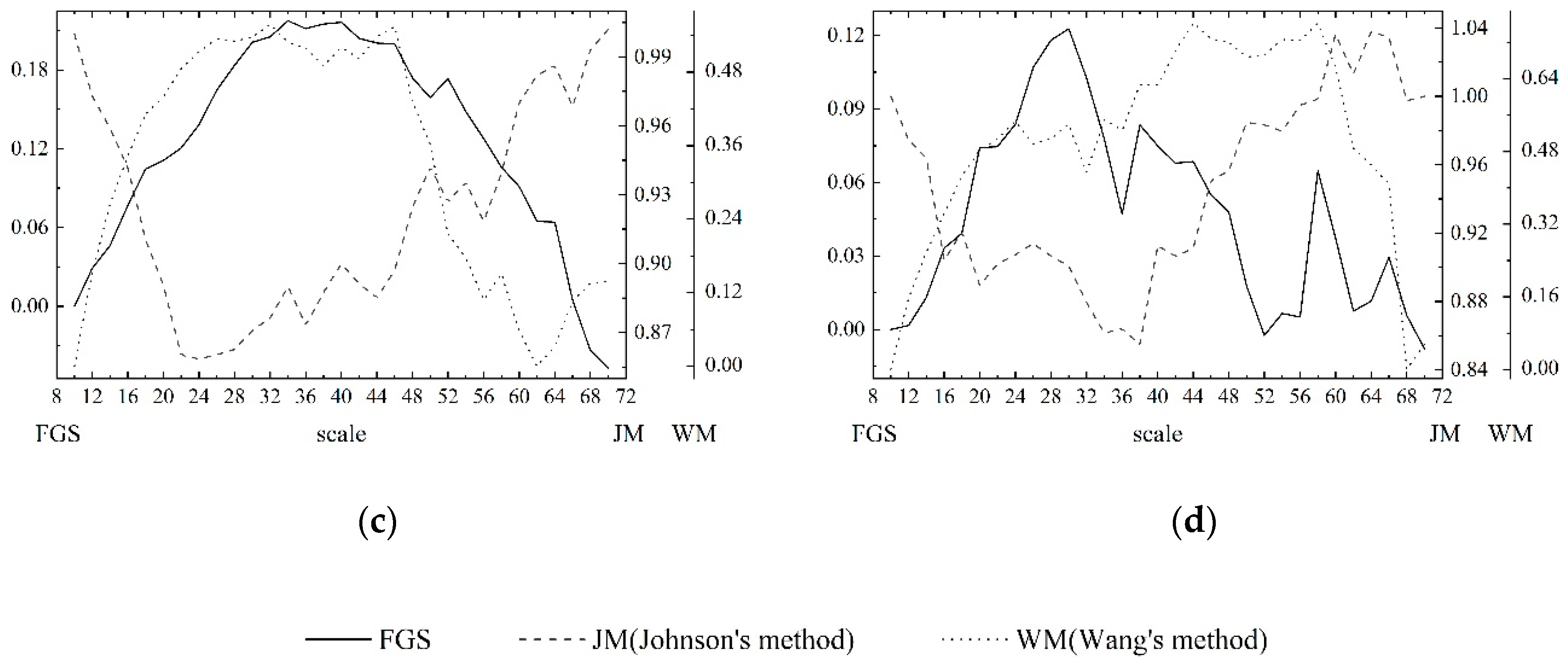
3.2. Effectiveness Analysis of FGS

To further prove the effectiveness of FGS, this paper compared it with Johnson’s method (JM) [30] and Wang’s method (WM) [24]. Because FGS’s intra-segment homogeneity evaluation indicators are the same as them, the difference lies in the inter-segment heterogeneity evaluation indicators. Note that all three methods use the same normalization method, thus, the lower measure values in Johnson’s method (JM) indicate higher segmentation quality and the higher measure values in the FGS and Wang’s method (WM) indicate higher segmentation quality. The optimal results obtained by the three methods are shown in Figure 6. For the T1 image, the optimal segmentation using the three methods was obtained by using the scale at 30, 30, and 32, respectively. For the T2 image, the optimal segmentation using the three methods was obtained by using the scale at 24, 18, and 38, respectively. For the T3 image, the optimal segmentation using the three methods was obtained by using the scale at 34, 24, and 32, respectively. For the T4 image, the optimal segmentation using the three methods was obtained by using the scale at 30, 38, and 44, respectively.

The local details of the optimal segmentation results of the four study areas obtained by FGS, JM, and WM are shown in Figure 7. In the first subset of T1, the playground was segmented better in the FGS and JM result, and it was under-segmented in the WM result. In the second subset of T1, the results of the three methods were under-segmented, because the buildings were confused with some vegetation, and the result of WM was more under-segmented. In the first subset of T2, the FGS and JM had similar performance and the result of them was more over-segmented, but the result of WM showed the phenomenon of under segmentation locally. In the second subset of T2, the results were over-segmented in the FGS and JM results. In the WM result, buildings and vegetation were not effectively separated, and under-segmentation occurred. In the first subset of T3, the buildings were all over-segmented in the results of the three methods, but the FGS and WM performed better than JM. In the second subset of T3, the farmland was all over-segmented in the results of the three methods, but geographic objects in JM were more fragmented. In the two subsets of T4, the and WM performed better in segmenting farmland than FGS, although the results of the three methods were all over-segmented.

In order to quantitatively evaluate the effectiveness of FGS,

Table 2. The accuracy assessment measures results for the segmentations produced by the FGS and other existing two UE methods.

Test	Methods	Accuracy Assessment Measures
		QR	OS	US	D
T1	FGS	0.2875	0.0849	0.2255	0.1914
	Johnson’s method	0.2875	0.0849	0.2255	0.1914
	Wang’s method	0.3016	0.0839	0.2414	0.2012
T2	FGS	0.2843	0.2293	0.0856	0.1944
	Johnson’s method	0.4242	0.3913	0.0864	0.2974
	Wang’s method	0.2795	0.1319	0.1702	0.1909
T3	FGS	0.3281	0.1744	0.1894	0.2212
	Johnson’s method	0.3924	0.3271	0.1285	0.2697
	Wang’s method	0.3281	0.1744	0.1894	0.2212
T4	FGS	0.3237	0.2487	0.1184	0.2194
	Johnson’s method	0.2969	0.1171	0.2073	0.1978
	Wang’s method	0.2915	0.0830	0.2269	0.1929

shows the accuracy assessment results of the optimal segmentation for four study areas using the three methods. For the T1 image, the QR and D values of the WM methods were both higher than FGS and JM, thus, indicating that the FGS and JM had a better performance in the T1 result. From the value of OS and US, we can find that the result of WM was most under-segmented and the three methods were equivalent in over-segmentation. For the T2 image, the QR and D values of the WM methods were both lowest, indicating that the WM had the best performance. The QR and D values of the JM methods were both highest, indicating that the JM had the worst performance. The OS value of JM was much higher than FGS and WM, indicating that the result of JM was more over-segmented. The US value of WM was much higher than FGS and JM, indicating that the result of WM was more under-segmented. For the T3 image, FGS performed the same as WM, and the JM had the worst performance in the T2 result, because the QR and D values of the JM methods were both higher than FGS and WM. From the value of OS and US, we can find that the result of JM was more over-segmented and the result of FGS and WM was more under-segmented. For the T4 image, both QR and D values at the optimal scale obtained by WM were lower than FGS and JM, indicating the segmentation at the scale obtained by WM was better. From the value of OS, we can find that the result of FGS was most under-segmented and the result of WM had less over-segmentation. The US value of JM and WM was similar and much higher than that of FGS, indicating that the results of JM and WM were more under-segmented.

3.3. The Performance of FGS on Other Datasets

In order to evaluate the performance of FGS more effectively, Massachuetts Buildings Dataset was used [44], which can be obtained from the website (http://www.cs.toronto.edu/~vmnih/data/). The images in this dataset contain three multi-spectral bands (blue, green, and red) with a resolution of 1 m. In this paper, four images with the size of 1500 × 1500 were selected for the experiment (Figure 8). The optimal results obtained by the three methods are shown in Figure 9. For the T5 image, the optimal segmentation using the three methods was obtained by using the scale at 28, 24, and 34, respectively. For the T6 image, the optimal segmentation using the three methods was obtained by using the scale at 32, 32, and 28, respectively. For the T7 image, the optimal segmentation using the three methods was obtained by using the scale at 32, 44, and 28, respectively. For the T8 image, the optimal segmentation using the three methods was obtained by using the scale at 30, 28, and 26, respectively.

The accuracy assessment results of the optimal segmentation for four study areas using the three methods are presented in

Table 3. The accuracy assessment measurement results for the segmentations produced by the FGS and other existing two UE methods, using the Massachuetts Buildings Dataset.

Test	Methods	Accuracy Assessment Measures
		QR	OS	US	D
T5	FGS	0.6411	0.4502	0.3709	0.4589
	Johnson’s method	0.6503	0.5059	0.3185	0.4650
	Wang’s method	0.6371	0.3877	0.4307	0.4564
T6	FGS	0.6231	0.3828	0.4091	0.4437
	Johnson’s method	0.6231	0.3828	0.4091	0.4437
	Wang’s method	0.6206	0.4276	0.3622	0.4419
T7	FGS	0.6131	0.4192	0.3392	0.4351
	Johnson’s method	0.6116	0.3260	0.4345	0.4348
	Wang’s method	0.6276	0.4715	0.3036	0.4467
T8	FGS	0.6491	0.3881	0.4446	0.4658
	Johnson’s method	0.6439	0.4077	0.4181	0.4615
	Wang’s method	0.6465	0.4363	0.3924	0.4635

. For the T5 image, the performance of FGS lied between WM and JM, indicated by the lower QR and D values. The OS value of JM was highest, indicating that the result of JM was more over-segmented. The US value of WM was highest, indicating that the result of WM was more under-segmented. For the T6 image, FGS performed the same as JM, and both performed worse than WM, indicated by the lower QR and D values. From the value of OS and US, we can find that WM performed worse in over-segmentation and better in under-segmentation. For the T7 image, the QR and D values of the FGS were lower than WM and higher than JM, thus, indicating that the FGS performed better than WM and worse than JM. From the value of OS and US, we can find that the result of JM was most under-segmented and the result of WM was most over-segmented. For the T8 image, both QR and D values at the optimal scale obtained by FGS were higher than JM and WM, indicating the segmentation at the scale obtained by FGS was worst. From the value of OS and US, we can find that the result of WM was most over-segmented and the result of FGS was most under-segmented. In addition, the QR and D values were not much different on Massachuetts Buildings Dataset, indicating that the performance of the three methods was very similar.

3.4. Computational Cost

This paper uses T1 as an example to analyze the computational cost of FGS, JM, and WM, and the relationship with the total number of objects. Because the intra-segment homogeneity measures of the three methods of FGS, JM, and WM are the same and the difference is the inter-segment heterogeneity measure, the computing efficiency of DTNP, MI, and BSH also reflects the efficiency of the three UE methods. Please note that all three measures of inter-segment heterogeneity were computed under the environment of eCognition Developer 9.0. DTNP, MI, BSH and the total number of objects at different scales of T1 are shown in Figure 10. As the scale increases, the number of objects obtained by segmentation decreases geometrically. The computational cost of DTNP, MI and BSH is positively correlated with the number of objects, and the correlation coefficients are 0.9906, 0.9999 and 0.9999 respectively, P values are all less than 0.05. Under the same scale, DTNP has the least computational cost, far less than MI and BSH. Therefore, FGS has the least computational cost compared with JM and WM.

4. Discussion

With the development of aviation and aerospace remote sensing technology, high-resolution remote sensing images containing more detailed spatial information are increasingly used. In order to make better use of spatial details, image segmentation is an indispensable processing step. The quality of image segmentation directly affects the accuracy of subsequent analysis, so it is important to evaluate image segmentation. Although the SE method can provide more accurate results, it requires manual generation of reference objects, which makes it difficult to be widely used in practical applications. The UE method can objectively evaluate the segmentation results without prior knowledge. Compared with SE, UE can not only be used for comparison and selection of segmentation methods, and the setting of segmentation parameters, but also for segmentation parameters optimization. Therefore, the UE method has gained more attention.

This study proposed the FGS combining intra-heterogeneity and inter-homogeneity to evaluate image segmentation. Compared with the existing UE method, FGS uses the same inter-segment heterogeneity evaluation measure, but creatively uses DTNP as the inter-segment heterogeneity measure. As the scale increases, the inter-segment heterogeneity also increases. The DTNP curve shown in Figure 8 can clearly reveal the process of increasing heterogeneity. FGS is always low when over- or under-segmented. The FGS curve shown in Figure 6 can clearly reveals the change from under-segmentation to optimal segmentation results and under-segmentation.

DTNP was proposed to measure inter-segment heterogeneity quickly and effectively. Through qualitative analysis of three inter-segment heterogeneity measures (Figure 5), we found that the BSH had a higher separability and MI had a lower separability in segmentation results, but the result was also most over-segmented in BSH result. Through quantitative analysis of three inter-segment heterogeneity measures (Table 1), we found that the QR and D values of DTNP were the lowest in the T1 and T3, the same as MI and were both lower than BSH in the T3, and the highest in the T4, thus, indicating that DTNP has comparable performance to MI and BSH as the inter-segment heterogeneity measure. Furthermore, the OS value of BSH was highest and the US value of BSH was lowest in four study areas, indicating that BSH performs best in under-segmentation but worst in over-segmentation. The OS value of MI was lowest and the US value of MI was highest in four study areas, indicating that MI performs best in over-segmentation but worst in under-segmentation. From the value of OS and US, we can find that DTNP can perform better than BSH on over-segmentation and better than MI on under-segmentation. Therefore, compared to MI and BSH, which are more sensitive to over-segmentation or under-segmentation, DTNP can keep stability and remain sensitive to both over-segmentation and under-segmentation.

To further prove the effectiveness of the proposed FGS, we compared it with JM and WM. The qualitative results (Figure 7) show that the segmentation results determined by the three methods can distinguish different geographic objects, but cannot accurately distinguish all geographic objects, because a single segmentation scale is not applicable to all geographic objects. Therefore, it is necessary to further study the optimization of segmentation parameters. The QR and D in the qualitative results (Table 2) indicate that FGS does not always perform better than the JM and WM methods. However, in the quantitative results of T1 and T3 images, the QR and D values of FGS were the lowest, indicating that FGS performs best. The experiment on Massachuetts Buildings Dataset demonstrates that the performance of FGS is similar to that of the compared method, and it can effectively evaluate the segmentation quality.

From the value of QR and D in Table 1 and Table 2, we can find that the quality of the segmentation results obtained by determining the optimal segmentation scale only through the evaluation of inter-segment heterogeneity was worse than that of the segmentation results obtained by determining the optimal segmentation scale through combining the evaluation of intra-segment homogeneity and inter-segment heterogeneity, which indicates the importance of intra-segment homogeneity and inter-homogeneity in segmentation quality evaluation.

From the result of computational cost, we can find that the computational cost of DTNP was much less than that of MI and BSH, and the computational cost of BSH was more than that of MI. DTNP need not construct RAG and computes with neighborhood objects, which lead the result of less computational cost. The computation process of BSH needs to use RAG twice, but it cannot be stored in the eCognition environment. Therefore, the computational cost of BSH is significantly increased by the two construction processes of RAG. If MI and BSH are computed by programming, the difference in computational cost will be greatly reduced. Note that the correlation coefficient between the computational cost of BSH and the number of objects is the lowest, because the number of objects is too few and the computational cost is too low, so it is difficult to make full use of computing resources. Since the computational cost of the heterogeneity in UE is more than the computational cost of other steps, we can infer from the computational cost of DTNP, MI, and BSH that the computational cost of FGS is much less than JM and WM.

5. Conclusions

The FGS based on WV and DTNP was proposed to evaluate the remote sensing image segmentation. The innovation of this study is to use the pixels of the object neighborhood as the inter-segment heterogeneity computational object. Compared with the existing methods, the performance is similar and the computational cost is greatly reduced. The experimental results show DTNP can clearly reveal the process of increasing heterogeneity and FGS can clearly reveal the change from over-segmentation to optimal segmentation results and under-segmentation. Furthermore, compared to MI and BSH, DTNP can keep stability and remain sensitive to both over-segmentation and under-segmentation. FGS has the similar performance with JM and WM but has the least computational cost. This advantage is more prominent when the UE method is applied to segmentation parameter optimization. The result in Section 3.1 and Section 3.2 indicates both homogeneity and heterogeneity play an important role in segmentation evaluation. This method can be effectively used in GEOBIA. In future research, more effective and time-consuming unsupervised evaluation methods should be studied and effectively applied to segmentation parameter optimization.

References

1. Chen, F.; Chen, X.; Van de Voorde, T.; Roberts, D.; Jiang, H.; Xu, W. Open water detection in urban environments using high spatial resolution remote sensing imagery. Remote Sens. Environ. 2020, 242, 111706. [Google Scholar] [CrossRef]
2. Wang, S.; Yang, H.; Wu, Q.; Zheng, Z.; Wu, Y.; Li, J. An Improved Method for Road Extraction from High-Resolution Remote-Sensing Images that Enhances Boundary Information. Sensors 2020, 20, 2064. [Google Scholar] [CrossRef] [PubMed] [Green Version]
3. Wu, T.; Luo, J.; Zhou, Y.n.; Wang, C.; Xi, J.; Fang, J. Geo-Object-Based Land Cover Map Update for High-Spatial-Resolution Remote Sensing Images via Change Detection and Label Transfer. Remote Sens. 2020, 12, 174. [Google Scholar] [CrossRef] [Green Version]
4. Zhang, L.; Wu, J.; Fan, Y.; Gao, H.; Shao, Y. An Efficient Building Extraction Method from High Spatial Resolution Remote Sensing Images Based on Improved Mask R-CNN. Sensors 2020, 20, 1465. [Google Scholar] [CrossRef] [PubMed] [Green Version]
5. Thomas, N.; Hendrix, C.; Congalton, R.G. A comparison of urban mapping methods using high-resolution digital imagery. Photogramm. Eng. Remote Sens. 2003, 69, 963–972. [Google Scholar] [CrossRef]
6. Myint, S.W.; Gober, P.; Brazel, A.; Grossman-Clarke, S.; Weng, Q. Per-pixel vs. object-based classification of urban land cover extraction using high spatial resolution imagery. Remote Sens. Environ. 2011, 115, 1145–1161. [Google Scholar] [CrossRef]
7. Huang, L.; Ni, L. Object-oriented classification of high resolution satellite image for better accuracy. In Proceedings of the 8th International Symposium Spatial Accuracy Assessement Natural Resources Environironmental Science Vol Ii: Accuracy Geomaterials, Shanghai, China, 25–27 June 2008; pp. 211–218. [Google Scholar]
8. Hossain, M.D.; Chen, D. Segmentation for Object-Based Image Analysis (OBIA): A review of algorithms and challenges from remote sensing perspective. ISPRS J. Photogramm. Remote Sens. 2019, 150, 115–134. [Google Scholar] [CrossRef]
9. Blaschke, T. Object based image analysis for remote sensing. ISPRS J. Photogramm. Remote Sens. 2010, 65, 2–16. [Google Scholar] [CrossRef] [Green Version]
10. Karlson, M.; Reese, H.; Ostwald, M. Tree Crown Mapping in Managed Woodlands (Parklands) of Semi-Arid West Africa Using WorldView-2 Imagery and Geographic Object Based Image Analysis. Sensors 2014, 14, 22643–22669. [Google Scholar] [CrossRef]
11. Zhang, X.; Feng, X.; Xiao, P.; He, G.; Zhu, L. Segmentation quality evaluation using region-based precision and recall measures for remote sensing images. ISPRS J. Photogramm. Remote Sens. 2015, 102, 73–84. [Google Scholar] [CrossRef]
12. Hernandez, I.E.R.; Shi, W. A Random Forests classification method for urban land-use mapping integrating spatial metrics and texture analysis. Int. J. Remote Sens. 2018, 39, 1175–1198. [Google Scholar] [CrossRef]
13. Goncalves, J.; Pocas, I.; Marcos, B.; Mucher, C.A.; Honrado, J.P. SegOptim—A new R package for optimizing object-based image analyses of high-spatial resolution remotely-sensed data. Int. J. Appl. Earth Obs. Geoinf. 2019, 76, 218–230. [Google Scholar] [CrossRef]
14. Chen, L.C.; Papandreou, G.; Kokkinos, I.; Murphy, K.; Yuille, A.L. DeepLab: Semantic Image Segmentation with Deep Convolutional Nets, Atrous Convolution, and Fully Connected CRFs. IEEE Trans. Pattern Anal. Mach. Intell. 2018, 40, 834–848. [Google Scholar] [CrossRef] [PubMed]
15. Kemker, R.; Salvaggio, C.; Kanan, C. Algorithms for semantic segmentation of multispectral remote sensing imagery using deep learning. ISPRS J. Photogramm. Remote Sens. 2018, 145, 60–77. [Google Scholar] [CrossRef] [Green Version]
16. Li, D.R.; Zhang, G.F.; Wu, Z.C.; Yi, L.N. An Edge Embedded Marker-Based Watershed Algorithm for High Spatial Resolution Remote Sensing Image Segmentation. IEEE Trans. Image Process. 2010, 19, 2781–2787. [Google Scholar] [CrossRef] [PubMed]
17. Vincent, L.; Soille, P. Watersheds in Digital Spaces: An Efficient Algorithm Based on Immersion Simulations. IEEE Trans. Pattern Anal. Mach. Intell. 1991, 13, 583–598. [Google Scholar] [CrossRef] [Green Version]
18. Shafarenko, L.; Petrou, M.; Kittler, J. Automatic watershed segmentation of randomly textured color images. IEEE Trans. Image Process. 1997, 6, 1530–1544. [Google Scholar] [CrossRef]
19. Eddy, P.R.; Smith, A.M.; Hill, B.D.; Peddle, D.R.; Coburn, C.A.; Blackshaw, R.E. Hybrid segmentation—Artificial Neural Network classification of high resolution hyperspectral imagery for Site-Specific Herbicide Management in agriculture. Photogramm. Eng. Remote Sens. 2008, 74, 1249–1257. [Google Scholar] [CrossRef]
20. Yang, J.; He, Y.H.; Caspersen, J. Region merging using local spectral angle thresholds: A more accurate method for hybrid segmentation of remote sensing images. Remote Sens. Environ. 2017, 190, 137–148. [Google Scholar] [CrossRef]
21. Liu, J.H.; Pu, H.; Song, S.R.; Du, M.Y. An adaptive scale estimating method of multiscale image segmentation based on vector edge and spectral statistics information. Int. J. Remote Sens. 2018, 39, 6826–6845. [Google Scholar] [CrossRef]
22. Wang, Y.J.; Qi, Q.W.; Liu, Y. Unsupervised Segmentation Evaluation Using Area-Weighted Variance and Jeffries-Matusita Distance for Remote Sensing Images. Remote Sens. 2018, 10, 1193. [Google Scholar] [CrossRef] [Green Version]
23. Shen, Y.; Chen, J.Y.; Xiao, L.; Pan, D.L. Optimizing multiscale segmentation with local spectral heterogeneity measure for high resolution remote sensing images. ISPRS J. Photogramm. Remote Sens. 2019, 157, 13–25. [Google Scholar] [CrossRef]
24. Wang, Y.J.; Qi, Q.W.; Liu, Y.; Jiang, L.L.; Wang, J. Unsupervised segmentation parameter selection using the local spatial statistics for remote sensing image segmentation. Int. J. Appl. Earth Obs. Geoinf. 2019, 81, 98–109. [Google Scholar] [CrossRef]
25. Zhang, H.; Fritts, J.E.; Goldman, S.A. Image segmentation evaluation: A survey of unsupervised methods. Comput. Vis. Image Underst. 2008, 110, 260–280. [Google Scholar] [CrossRef] [Green Version]
26. Clinton, N.; Holt, A.; Scarborough, J.; Yan, L.; Gong, P. Accuracy Assessment Measures for Object-based Image Segmentation Goodness. Photogramm. Eng. Remote Sens. 2010, 76, 289–299. [Google Scholar] [CrossRef]
27. Liu, Y.; Bian, L.; Meng, Y.H.; Wang, H.P.; Zhang, S.F.; Yang, Y.N.; Shao, X.M.; Wang, B. Discrepancy measures for selecting optimal combination of parameter values in object-based image analysis. ISPRS J. Photogramm. Remote Sens. 2012, 68, 144–156. [Google Scholar] [CrossRef]
28. Yang, J.; He, Y.H.; Weng, Q.H. An Automated Method to Parameterize Segmentation Scale by Enhancing Intrasegment Homogeneity and Intersegment Heterogeneity. IEEE Geosci. Remote Sens. Lett. 2015, 12, 1282–1286. [Google Scholar] [CrossRef]
29. Espindola, G.M.; Camara, G.; Reis, I.A.; Bins, L.S.; Monteiro, A.M. Parameter selection for region-growing image segmentation algorithms using spatial autocorrelation. Int. J. Remote Sens. 2006, 27, 3035–3040. [Google Scholar] [CrossRef]
30. Johnson, B.; Xie, Z.X. Unsupervised image segmentation evaluation and refinement using a multi-scale approach. ISPRS J. Photogramm. Remote Sens. 2011, 66, 473–483. [Google Scholar] [CrossRef]
31. Yang, J.; Li, P.J.; He, Y.H. A multi-band approach to unsupervised scale parameter selection for multi-scale image segmentation. ISPRS J. Photogramm. Remote Sens. 2014, 94, 13–24. [Google Scholar] [CrossRef]
32. Gao, H.; Tang, Y.; Jing, L.; Li, H.; Ding, H. A Novel Unsupervised Segmentation Quality Evaluation Method for Remote Sensing Images. Sensors 2017, 17, 2427. [Google Scholar] [CrossRef] [PubMed]
33. Haralick, R.M.; Shapiro, L.G. Image Segmentation Techniques. Comput. Vis. Graph. Image Process. 1985, 29, 100–132. [Google Scholar] [CrossRef]
34. Xiong, Z.Q.; Zhang, X.Y.; Wang, X.N.; Yuan, J. Self-adaptive segmentation of satellite images based on a weighted aggregation approach. GIScience Remote Sens. 2019, 56, 233–255. [Google Scholar] [CrossRef]
35. Levine, M.D.; Nazif, A.M. Dynamic Measurement of Computer Generated Image Segmentations. IEEE Trans. Pattern Anal. Mach. Intell. 1985, 7, 155–164. [Google Scholar] [CrossRef]
36. Woodcock, C.E.; Strahler, A.H. The Factor of Scale in Remote-Sensing. Remote Sens. Environ. 1987, 21, 311–332. [Google Scholar] [CrossRef]
37. Vamsee, A.M.; Kamala, P.; Martha, T.R.; Kumar, K.V.; Sankar, G.J.; Amminedu, E. A Tool Assessing Optimal Multi-Scale Image Segmentation. J. Indian Soc. Remote Sens. 2018, 46, 31–41. [Google Scholar] [CrossRef]
38. Yin, R.J.; Shi, R.H.; Gao, W. Automatic Selection of Optimal Segmentation Scales for High-resolution Remote Sensing Images. In Proceedings of the Conference on Remote Sensing and Modeling of Ecosystems for Sustainability X, San Diego, CA, USA, 24 September 2013. [Google Scholar] [CrossRef]
39. Johnson, B.A.; Bragais, M.; Endo, I.; Magcale-Macandog, D.B.; Macandog, P.B.M. Image Segmentation Parameter Optimization Considering Within—And Between-Segment Heterogeneity at Multiple Scale Levels: Test Case for Mapping Residential Areas Using Landsat Imagery. ISPRS Int. J. Geo Inf. 2015, 4, 2292–2305. [Google Scholar] [CrossRef] [Green Version]
40. eCognition Software. Available online: https://geospatial.trimble.com/products-and-solutions/ecognition (accessed on 11 September 2020).
41. Sun, W.; Chen, B.; Messinger, D.W. Nearest-neighbor diffusion-based pan-sharpening algorithm for spectral images. Opt. Eng. 2013, 53, 013107. [Google Scholar] [CrossRef] [Green Version]
42. ENVI Software. Available online: https://www.harris.com/solution/envi (accessed on 11 September 2020).
43. Benz, U.C.; Hofmann, P.; Willhauck, G.; Lingenfelder, I.; Heynen, M. Multi-resolution, object-oriented fuzzy analysis of remote sensing data for GIS-ready information. ISPRS J. Photogramm. Remote Sens. 2004, 58, 239–258. [Google Scholar] [CrossRef]
44. Mnih, V. Machine Learning for Aerial Image Labeling; University of Toronto: Toronto, ON, Canada, 2013. [Google Scholar]
Figure 1. Schematic of the proposed method for segmentation evaluation.
Remotesensing 12 03005 g001
Figure 2. Four typical study areas of the GF-2 image: (a) T1, residential area; (b) T2, industrial area; (c) T3, mixed areas of residential areas, industrial areas, and farmland; and (d) T4, farmland area. Green polygons represent the manually digitized reference.
Remotesensing 12 03005 g002
Figure 3. The surrounding area of object i defined by its bounding box with the distance of one pixel.
Remotesensing 12 03005 g003
Figure 4. The H ˙ , I, and normalized results of difference to neighbor pixels (DTNP), Moran’s I (MI), and between-segment heterogeneity (BSH) of four test images.
Remotesensing 12 03005 g004
Figure 5. Subsets of the optimal segmentation for four test images obtained by the DTNP and other existing two inter-segment heterogeneity methods.
Remotesensing 12 03005 g005aRemotesensing 12 03005 g005b
Figure 6. The unsupervised evaluation (UE) results of the segmentations produced by the different UE methods for the four study areas: (a) T1, (b) T2, (c) T3, and (d) T4.
Remotesensing 12 03005 g006aRemotesensing 12 03005 g006b
Figure 7. Subsets of the optimal segmentation for four test images obtained by the fast-global score (FGS) and other existing two UE methods.
Remotesensing 12 03005 g007aRemotesensing 12 03005 g007b
Figure 8. Four images in Massachuetts Buildings Dataset: (a) T5, (b) T6, (c) T7, and (d) T8. Green polygons represent the reference of buildings.
Remotesensing 12 03005 g008aRemotesensing 12 03005 g008b
Figure 9. The UE results of the segmentations produced by the different UE methods for the Massachuetts Buildings Dataset: (a) T5, (b) T6, (c) T7, and (d) T8.
Remotesensing 12 03005 g009
Figure 10. Execution time of three inter-segment heterogeneity methods and object number at different scales.
Remotesensing 12 03005 g010