Article

Vegetation Carbon Sequestration Mapping in Herbaceous Wetlands by Using a MODIS EVI Time-Series Data Set: A Case in Poyang Lake Wetland, China

1
State Key Laboratory of Hydrology-Water Resources and Hydraulic Engineering, Hohai University, Nanjing 210098, China
2
College of Hydrology and Water Resources, Hohai University, Nanjing 210098, China
3
Key Laboratory of Watershed Geographic Sciences, Nanjing Institute of Geography and Limnology, Chinese Academy of Sciences, Nanjing 210008, China
4
University of Chinese Academy of Sciences, Beijing 100049, China
5
Department of Geography, Ohio State University, Columbus, OH 43210, USA
*
Author to whom correspondence should be addressed.
Remote Sens. 2020, 12(18), 3000; https://doi.org/10.3390/rs12183000
Submission received: 28 July 2020 / Revised: 11 September 2020 / Accepted: 13 September 2020 / Published: 15 September 2020
(This article belongs to the Special Issue Remote Sensing of Wetlands)

Abstract

:
The carbon sequestration capacity of wetland vegetation determines carbon stocks and changes in wetlands. However, modeling vegetation carbon sequestration of herbaceous wetlands is still problematic due to complex hydroecological processes and rapidly changing biomass carbon stocks. Theoretically, a vegetation index (VI) time series can retrieve the dynamic of biomass carbon stocks and could be used to calculate the cumulative composite of biomass carbon stocks during a given interval, i.e., vegetation carbon sequestration. Hence, we explored the potential for mapping vegetation carbon sequestration in herbaceous wetlands in this study by using a combination of remotely sensed VI time series and field observation data. This method was exemplarily applied for Poyang Lake wetland in 2016 by using a 16-day Moderate Resolution Imaging Spectroradiometer (MODIS) enhanced vegetation index (EVI) time series. Results show that the vegetation carbon sequestration in this area was in the range of 193–1221 g C m−2 year−1 with a mean of 401 g C m−2 year−1 and a standard deviation of 172 g C m−2 year−1 in 2016. The approach has wider spatial applicability in wetlands than the currently used global map of vegetation production (MOD17A3) because our carbon estimation in areas depicted by ‘no data’ in the MOD17A3 product is considerable, which accounts for 91.2–91.5% of the total vegetation carbon sequestration of the wetland. Thus, we determined that VI time series data shows great potential for estimating vegetation carbon sequestration in herbaceous wetlands, especially with the continuously improving quality and frequency of satellite VI images.

Graphical Abstract

1. Introduction

Vegetation carbon sequestration is the amount of carbon that can be sequestered by vegetation during a given interval. It is the main carbon input of ecosystems [1]. Monitoring and reporting vegetation carbon sequestration in wetlands are important tasks [2] because climate change has become an indisputable fact [3,4], and the wetland carbon pool is one of the most important carbon sinks in regional ecosystems [5].
Extensive studies were conducted to estimate vegetation carbon sequestration in wetlands on various spatial scales. At a site scale, scientists collect data at a sufficient number of intervals to capture variation in biomass carbon stocks; the positive differences across annual collection dates are referred to as the yearly carbon sequestration of plants. For example, Pierfelice et al. [6] calculated the monthly fluctuations in biomass carbon stocks at three wetland sites in South Carolina in 2010–2012 to estimate the yearly vegetation carbon sequestration. Peregon et al. [7] monitored the maximum and minimum seasonal weights of biomass carbon stocks in Western Siberia and used their difference to estimate the vegetation carbon sequestration. Caplan et al. [8] summed the daily turnovers of biomass carbon stock simulated by an empirical plant growth model to yield the vegetation carbon sequestration in Edgewater, MD, USA. Additionally, the eddy covariance technique is also widely used on small spatial scales to calculate the levels of vegetation carbon sequestration [9]. It measures the covariance between fluctuations in vertical wind velocity and the CO2 mixing ratio, which produces estimations of RE (ecosystem respiration) and NEE (net ecosystem exchange) and hence the vegetation carbon sequestration [9].
For larger regional scales, vegetation carbon sequestration can be measured using two methods as follows: (1) extrapolating the field-measured carbon sequestration values up to a large region according to a vegetation map [7,10] and (2) utilizing satellite data-driven models based on ecophysiological process theories [11,12]. The accuracy of the former depends mainly on the number of categories displayed on the vegetation map [7,10]. Moreover, the spatial extrapolation method ignores the individual differences in the growth rate of the same species due to microenvironmental conditions [13]. For the satellite data-driven ecophysiological process models, the coarse meteorological data usually limit the spatial resolution [14]. Parameterizing these empirical relationships in ecophysiological processes over wide-ranging climatic and vegetation types is also problematic [15,16,17]. For example, the most widely used global-scale estimation of vegetation production, termed MOD17A3 [18,19], contains significant errors because of the use of coarse resolution weather data and the ‘Look-Up Table’-based ecophysiological inputs [17,20].
To avoid uncertainties in the spatial extrapolation method and ecophysiological process models, several scholars have attempted to use simple models based entirely on remote sensing data to estimate vegetation carbon sequestration on regional scales [21,22,23]. A significant correlation was found between field-measured vegetation carbon sequestration and a remotely sensed vegetation index (VI) in various environments. For example, Rahman et al. [22] revealed a strong correlation between vegetation carbon sequestration and enhanced vegetation index (EVI) in areas with wide-ranging vegetation types in North America. Sjöström et al. [23] found that EVI correlates well with estimated vegetation carbon sequestration on a site-by-site basis across various African ecosystems. Almost all these insight studies revealed that a straightforward, remotely sensed per-pixel input regression model shows potential to become an alternative method for estimating vegetation carbon sequestration on a regional scale. However, vegetation carbon sequestration is the cumulative value of biomass carbon stocks in a given interval. These studies only used a few VI images acquired at a particular time to retrieve the annual vegetation carbon sequestration and had ignored the dynamic nature of biomass carbon stocks.
Moreover, the current estimation methods for vegetation carbon sequestration are not suitable for herbaceous wetlands on small and large scales. On a small scale, the method of estimating vegetation carbon sequestration with high-frequency observations of biomass carbon stock is impractical in herbaceous wetlands, especially for the remote, inaccessible and dangerous locations [24,25]. On a regional scale, most satellite data-driven models are based on ecophysiological processes in terrestrial environments (forests and farmlands) [11,12,14,15,16,17]. Thus, these models cannot assess the key factors, such as the hydraulic forces of flooding and drawdown, which control the carbon cycle of wetland vegetation [26,27]. Additionally, the rapid changes in biomass carbon stocks in herbaceous wetlands have limited the practical use of current remote sensing-based regression models [21,22,23] because they utilize only small amounts of VI images acquired during specific periods throughout the growing season.
Theoretically, a VI time series at a sufficient number of intervals can directly provide consistent temporal comparisons of biomass carbon stocks on a regional scale. By utilizing a high-frequency VI time series to retrieve the rapid dynamics of biomass carbon stocks in herbaceous wetlands over a year, we could accurately estimate their yearly vegetation carbon sequestration. However, the feasibility of this assumption has long been limited by two issues. The first is the ability of VIs in estimating biomass carbon stocks, and the second is the frequency of VI time series in describing the continuous dynamics of biomass carbon stocks. Fortunately, recent research advances about these two issues have made the assumption feasible.
Firstly, the ability of VIs in estimating biomass carbon stocks is improving. VI is generated on the physical basis of the difference of plant leaves in reflectance in the red and near infrared (NIR) bands in optical remote sensing and has been widely used to evaluate biomass carbon stocks. Over 40 VIs have been developed during the past two decades [28,29,30], such as the normalized difference vegetation index, soil adjusted vegetation index, atmospherically resistant vegetation index, and EVI [31,32,33]. These VIs have improved the accuracy of biomass carbon stock estimation to varying degrees, especially for EVI. Additionally, with the development of hyperspectral remote sensing and infrared remote sensing, some new VIs such as Hyp_NDVI have been proposed [34]. These VIs are calculated from the red edge and NIR shoulder domains and can more accurately estimate biomass carbon stocks at full canopy cover than the standard red/NIR indices [34,35,36]. However, the use of fine spectral resolution sensors (more than 100 bands) is heavily limited in terms of cost, availability, and complexity of processing the high dimensional data, especially in wetlands covering large areas [36]. In summary, the atmospheric- and soil-corrected VIs generated from the moderate-spectral-resolution sensors, such as the EVI, are the most common and well-tested methods for biomass carbon stock estimation over a large wetland region.
Secondly, the improvement in the revisit frequency of the satellite missions allows the VI time series to capture further details of biomass carbon stock fluctuations [37,38]. For example, daily observations of VI are available provided by the Moderate Resolution Imaging Spectroradiometer (MODIS) instruments with a spatial resolution of 250 m (https://modis.ornl.gov). With a 30 m spatial resolution, Landsat satellites can achieve a 16-day revisit period. Moreover, Sentinel satellites can achieve a 5-day revisit period with a spatial resolution of 10–20 m (https://www.sentinel-hub.com). However, only high-frequency observations can obtain enough cloud-free VI images due to the cloudy and rainy weather for most herbaceous wetlands. For example, the 16 day Landsat product only captured five cloud-free images in 2009 in the largest freshwater wetland in China, i.e., the Poyang Lake wetland. Although the cloud contamination also causes disturbances in the daily MODIS VI time series, such noises have been greatly reduced in the 16 day maximum value composite products synthesized from the daily MODIS VI images, i.e., MOD13Q1 [39]. Additionally, various noise-reduction methods for reconstructing high-quality VI time-series data sets have been formulated, applied, and evaluated in the last two decades [40,41,42,43]. These methods can be broadly divided into four groups: (1) threshold-based methods such as the best index slope extraction algorithm [44]; (2) Fourier-based fitting methods [45] such as Sellers et al.’s [46] fast Fourier transform method; (3) asymmetric function fitting methods such as the double logistic method [43]; and (4) alternative filtering techniques such as the adaptive Savitzky-Golay filter [41]. Most of these methods have good performances, and the reconstructed VI time series are of high quality and have been further used in many aspects, such as detecting long-term land-use/cover changes [47], monitoring the phenological dynamics of vegetation [48], and classifying vegetation or land cover types [49].
In view of the continuous improvements of the quality and frequency of satellite VI time series currently, we tested our assumption of measuring vegetation carbon sequestration by a reconstructed VI time series and field observation data in a typical herbaceous wetland of Poyang Lake, China in this study. Specifically, we selected the 16 day MODIS EVI time series data set of 2016 in this wetland as the original VI time series. The Savitzky-Golay filter then reconstructed a new high quality EVI time series from the original one. The new reconstructed EVI time series along with its corresponding field vegetation data subsequently estimated the dynamics of biomass carbon stocks. This estimation was then used to calculate the cumulative composite of biomass carbon stocks in the year, i.e., the vegetation carbon sequestration in 2016. The accuracy of this method was evaluated by comparing it with the results of previous studies and the current global vegetation productivity map, i.e., the MOD17A3, in this wetland.

2. Materials and Methods

2.1. Study Area

Our study area was the Poyang Lake wetland (115°49′ E–116°46′ E, 28°24′ N–29°46′ N) at the southern bank of the middle reaches of the Yangtze River, China (Figure 1a). The climate in this region is typically warm (annual mean temperature ranging from 16.5 to 17.8 °C), humid (annual mean precipitation ranging from 1400 to 1700 mm), and prone to monsoons (annual water level amplitude averaging up to 11 m) [50]. Thus, the water regime of Poyang Lake follows a typical seasonal variation with the lake water rising in spring, flooding in summer, retreating in autumn, and drying in winter. The summer flood season generally lasts from June to September when the lake covers an area of 3800 km2 and inundates most of the low-lying alluvial plains surrounding the lake [51]. The prolonged inundation period provides inability for the trees to survive in this wetland. Thus, Poyang Lake is a typical herbaceous wetland [52].
The biota of this wetland shows a clear belt structure along the coastline due to its topography and water regime gradients [52]. Two types of herbaceous vegetation, i.e., semiaquatic emergent tall vegetation (composed mainly by Phragmites spp.) and emergent aquatic vegetation (composed mainly by Carex spp.), colonize the lake borders at various elevations (Figure 1c) [26,27].
The Phragmites community, which mainly includes Phragmites spp. and Triarrhena lutarioriparia L. Liu, is the most abundant vegetation type in the semiaquatic emergent tall vegetation zone. These plants colonize the high wetland areas, which can be flooded for at most 2 months in a year [53]. The growing season of plants in this zone begins in early spring, peaks in summer, and ends in late autumn.
The Carex community, which mainly includes Carex cinerascens Kṻkenth, Carex argyi Level. et Vaniot, and Carex unisexualis C. B. Clarke, is the most abundant in the emergent aquatic vegetation zone. These plants colonize the low wetland areas, which can be flooded for up to 160 days [53]. Therefore, the growing season of plants in this zone is divided into two stages by the long-lasting summer floods. The first stage happens in spring before the summer flooding, and the second occurs in autumn after the summer flooding. In summer, the plants in the Carex community become completely inundated and go into a dormancy phase.
Figure 1b is the land cover map of Poyang Lake wetland in 2016 that was remotely interpreted by Dai [54]. This figure identifies the two main kinds of herbaceous plants and shows their distribution across the entire wetland.

2.2. Data Collection and Processing

The VI time series-based method for estimating vegetation carbon sequestration in our study can be divided into five distinct steps, i.e., (1) preprocessing of the EVI time series and field observation data; (2) performing regression analyses between EVI values and the field-observed biomass carbon stocks; (3) retrieving the dynamics of biomass carbon stocks throughout the year by using the preprocessed EVI time series via the best estimation model; (4) estimating the annual vegetation carbon sequestration by using the retrieved dynamic of biomass carbon stocks; and (5) assessing the accuracy of the method by comparing it with other studies and the currently used global map of vegetation production (MOD17A3).

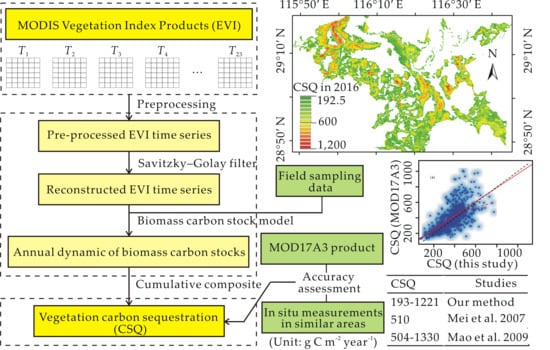
2.2.1. Vegetation Index Time Series Data and Preprocessing

The VI time series used in this study was the 23 scenes of MODIS EVI images acquired in 2016 and fully covering the Poyang Lake wetland. These scenes are extracted from the MODIS vegetation indices (NDVI and EVI) product suite (MODIS\Terra Vegetation Indices 16-Day L3 Global 250 m, MOD13Q1) produced on 16 day intervals [39]. An EVI time series should follow a smoothing cycle of growth and decline with the growth of plants within a year. However, clouds or poor atmospheric conditions usually depress the EVI values in the EVI time series. Thus, we performed three steps in our data preprocessing to generate a high-quality EVI time series with great temporal consistency.
  • Firstly, the images were coregistered and subset to the Poyang Lake wetland. The summary quality layer of MOD13Q1 was used to remove the low-quality values in the EVI images.
  • Then, we used a seasonal-trend decomposition method to further remove the outliers in the remaining values of the EVI time series from the aspect of temporal consistency. For further details, please refer to Cleveland et al. [55].
  • Next, we interpolated the discarded values in the abovementioned two steps via a Savitzky-Golay filter [56]. This filter is a simplified least squares-fit convolution for smoothing and computing the derivatives of a set of consecutive values. This filter has been widely used for VI time series reconstruction and showed great superiority over other methods [41,42,43].
Figure 2 illustrates the processing effect of the above three steps. The preprocessed EVI time series identified and corrected most of the noise. The general pattern of seasonal changes in the preprocessed EVI time series became evidently clear.

2.2.2. Field Sampling Plots

We used two sources of field-measured vegetation data in this study. One was the 86 plots (Source A in Figure 3) we gathered from the four subregions in the wetland during 24 November to 3 December 2016. The samples were collected from both the two main vegetation communities in this wetland, i.e., Phragmites community (6 samples) and Carex community (80 samples), and are located in all four different kinds of bottomlands, including littoral land of the main lake (41 samples), inflow river delta (14 samples), sublakes (24 samples), and small islands (7 samples). The other data were the 32 plots discussed in Wu et al.’s [57] study (Source B in Figure 3 gathered in northwest Poyang Lake wetland in September, October, and November during 2008–2011 coinciding with the satellite overpass).
In our survey, aboveground biomass in a 1 m × 1 m plot was harvested by clipping the plants at the soil level at each site. Wet biomass was weighed and then converted to dry biomass through a proportionality constant, i.e., the water content factor (taken as 0.3 via a sample analysis). Next, the dry biomass was converted to biomass carbon stock (g C m−2) through a carbon conversion factor ρ, which was taken as 0.44 in grass ecosystems [8,58]. In Wu et al.’s [57] study, plant biomass yields were also measured as the wet weight (g wet mass m−2). Thus, those records were also converted to biomass carbon stock by using the water content factor and carbon conversion factor [59].
For each field sampling plot, a handheld GPS receiver (GPS 60, GARMIN, Olathe, KS, USA) recorded the geographic coordinates, which were then used to extract the corresponding EVI values from the coincident MODIS EVI image by the ExtractValuesToPoints tools in ESRI ArcGIS 10.2 (Esri, Redlands, CA, USA). Sample points with the same sampling time and falling in the same MODIS pixel were averaged to coincide with the corresponding single MODIS EVI value. Through this process, 56 records can be finally used to train and verify the biomass carbon stock estimation model.

2.2.3. Biomass Carbon Stock Modeling

The biomass carbon stock estimation models were developed based on the regression analysis between the remotely sensed EVI and the field-observed biomass carbon stocks. All records were plotted in one scatter plot because of the limited small sample size (56 records). Records from different data sources were differently marked to check the consistency of the EVI-biomass carbon stock relationships at different acquiring times. Additionally, records from different data sources were used to intercalibrate each other in the biomass carbon stock modeling.
We tested four regression models, including the power law model (y = a·xb), exponential model (y = a·ebx), simple linear regression model (y = a·x + b), and polynomial model (y = a·x2 + b·x + c), to fit the curve according to the shape of the scatter plot. The ordinary least squares method was used to estimate the parameters of all four models, whereas the coefficient of determination (R2) was utilized to compare the errors of these models. The best fitting model was used to reconstruct the dynamics of biomass carbon stock throughout the year from the EVI time-series images.

2.2.4. Estimating the Annual Vegetation Carbon Sequestration

Basing on the reconstructed time profile of biomass carbon stock throughout the year, we calculated the annual vegetation carbon sequestration of each pixel via Equation (1). As a result, the sum of positive differences in biomass carbon stocks across collection dates during the year was determined.
C S Q = t = 1 22 k t ,   k t = { B i o . C t + 1 B i o . C t   ,   if   B i o . C t + 1 B i o . C t > 0 0   ,   otherwise  
where CSQ is the abbreviation of vegetation carbon sequestration and t is the varying integer that denotes the date of biomass carbon stock analysis. Given the 23 EVI images per year for the 16 day MODIS EVI time series data, the range of t is from 1 to 22. kt is the positive difference in biomass carbon stocks between adjacent dates, which is calculated by Bio.Ct, the biomass carbon stock observed at time t.

3. Results

3.1. Quality of the Processed EVI Time Series

The processed and raw EVI curves at 60 randomly selected pixels were compared to evaluate the quality of our preprocessed EVI time series. We also compared the reconstructed EVI curves by using the Savitzky–Golay filter and two other time series filtering methods, i.e., the asymmetric Gaussian method [42] and the double logistic method [43], to further examine the performances of the Savitzky–Golay filter. Only the results of 12 test pixels are shown in Figure 4 due to space limitations.
For the pixels of high quality, the processed EVI values of the Savitzky–Golay filter were closest to the original EVI values among those of the three methods. For the pixels of low quality, i.e., the excluded outliers, the processed EVI values of the Savitzky–Golay filter had the smoothest transition from neighboring points among those of the three methods. Thus, the Savitzky–Golay filter was the most effective for constructing EVI time-series data sets in this area among all of the three methods. By interpolating those excluded outliers by the Savitzky–Golay filter, we successfully identified and corrected most of the noisy points and generated a high quality EVI time series with great temporal consistency. Moreover, the processed EVI time profiles successfully captured the phenological variations of the two main vegetation types in Poyang Lake wetland. Specifically, plants in the Phragmites community ‘peak’ once in summer (Nos. 1–4), whereas plants in the Carex community ‘peak’ twice in spring and autumn (Nos. 5–12).

3.2. Modeling of Biomass Carbon Stock Estimation

Results of single regression analyses among all the EVI and field-observed biomass carbon stocks are illustrated in Figure 5, wherein the records from different data sources were differently marked. The best fit (R2 = 0.80, RMSE = 39.86 g C m−2) was obtained through the quadratic polynomial regression model (Model 4: y = 978.80x2 − 54.07x + 67.11, n = 56; Figure 5d). Moreover, the results indicated no significant change in the relationship between the field-observed biomass carbon stock and EVI at multiple data acquisition times (p < 0.01). Thus, we determined that in view of the greatly improved quality and temporal consistency of the EVI time series, the EVI-biomass carbon stock records obtained at different times in one regression model could be used to retrieve the annual dynamic of biomass carbon stock in this wetland with stable land-use and land-cover conditions.
To validate the quadratic polynomial model for biomass carbon stock estimation, we conducted an experiment to determine whether or not the independent samples from data source A and data source B would calibrate each other. Specifically, we established two models by using two sets of data via the well-fitting quadratic polynomial regression method as shown in Figure 6. The model established by data source A (data source B) was marked as model A (model B), which used the remaining data, i.e., the samples of data source B (data source A), for verification. The quadratic polynomial regression model (Model 4: y = 978.80x2 − 54.07x + 67.11, n = 56), which was trained by all the samples, was also illustrated in Figure 6 for comparison. As shown in Figure 6, the estimated biomass carbon stocks from model A (model B) could explain more than 70% of the variance of biomass carbon stocks derived from the ground survey in data source B (data source A; both R2 equal to 0.79), indicating that the survey data from different dates could intercalibrate each other.

3.3. Reconstructing the Annual Dynamic of Biomass Carbon Stocks

We utilized model 4, the most accurate quadratic polynomial regression model trained by all the ground samples, for the strictly preprocessed EVI time series to estimate the inner-annual variations of biomass carbon stock in Poyang Lake wetland in 2016 (Figure 7). From March until April, as time progresses the biomass carbon stocks increased gradually due to the sprout and rapid growth of vegetation during mid-late spring. After reaching the maximum value in mid-April, the biomass carbon stocks began to decrease, especially for the locations on the low-lying alluvial plains surrounding the lake. This decrease is mainly attributed to the Carex community on low surfaces. This community becomes dormant during early summer because water spreads over these surfaces and eventually covers the plants. During the fall after the lake recedes and the surfaces are exposed, the plants in the Carex community began their second growth period and grow vigorously. Thus, the biomass carbon stocks of the wetland increased again and peaked at early November. Moreover, given that all plants become dormant as winter approaches, the biomass carbon stocks of the wetland began to decrease in December.

3.4. Reported Annual Vegetation Carbon Sequestration from Different Biomass Carbon Stock Maps

In this section, the sum of the positive differences in biomass carbon stocks throughout the year, i.e., the annual vegetation carbon sequestration of the wetland, was finally estimated based on the reconstructed time profile of biomass carbon stocks. The average carbon sequestration of Poyang Lake wetland vegetation was 401 g C m−2 year−1 in 2016 with a standard deviation of 172 g C m−2 year−1 (Figure 8). Wide variations were observed in the vegetation carbon sequestration along the topographic gradient depending on the microhabitat that resulted from the water level fluctuations. In the area beside the central water surface, a widespread sparsely vegetated area was mixed with a mudflat due to the strong flooding stress. Thus, the vegetation in this area can only sequester a small amount of carbon. However, in the areas close to the edge of the wetland, the vegetation productivity rapidly increased to extremely high levels due to the mitigation of long-term immersion. Thus, vegetation in that area can sequester a large amount of carbon. The Nanjishan National Nature Reserve (NNNR) and the Wucheng National Nature Reserve (WNNR) are the two high-productive regions within the wetland and are located in the southwest and northwest parts of this area, respectively. The average value of vegetation carbon sequestration in the east NNNR in 2016 was 501 g C m−2 year−1, and that of the north WNNR was 750 g C m−2 year−1.

4. Discussion

4.1. Accuracy Assessment of the Output of the VI Time Series-Based Method

Few field studies have measured vegetation carbon sequestration in Poyang Lake wetland due to its dramatic water level fluctuations and high risk of Schistosoma infection [57]. Thus, a preliminary evaluation of the estimate of the VI time series-based method was conducted in two ways, namely, (1) comparing the results of previous studies for herbaceous wetlands in other areas of similar climate conditions and (2) comparing the model with the currently used global map of vegetation production (MOD17A3HGF Version 6 product).

4.1.1. Comparison of Vegetation Carbon Sequestration Estimates for Other Areas

We compared our vegetation carbon sequestration estimate in Poyang Lake wetland with those from two other study sites in China, namely, East Chongming wetland [60] and Yancheng coastal wetland [61], which are in a similar latitude with Poyang Lake wetland (Figure 1a). These estimates were obtained by in situ measurements and are summarized in Table 1. Besides, Table 1 also summarized the carbon sequestration difference between the two main vegetation types in the Poyang Lake wetland based on our estimates, which could help the cross-site comparison as well as to characterize the carbon sequestration differences between communities. Importantly, we see that in our estimates the regional average values of vegetation carbon sequestration are lower than the values extracted at the field sampling plots. This is because the areas that can be involved in sampling are generally with some distance from the water surface, thus they are easy to access and have a relatively high carbon sequestration ability. This explains why the estimates by in situ measurement from other studies are generally larger than our estimates for the whole wetland. For the sample-site values, however, the estimate from the study of Mei and Zhang [60] merely shows a slight bias against our estimate for Carex community (15 g C m−2 year−1). The estimate for the Herba suaedae site in Yancheng coastal wetland from the study of Mao et al. [61] is also in line with our estimate for the Carex community (9 g C m−2 year−1). However, the estimates of Mao et al. [61] for Scirpus triqueter and Phragmites spp. sites are higher than our estimate for the Phragmites community and approximately identical to the maximum value of our estimates, i.e., 1221 g C m−2 year−1. This phenomenon occurs because the growth area of S. triqueter and Phragmites spp. shows high production in Yancheng coastal wetland. Therefore, the in situ measurements of vegetation carbon sequestration at these sites should approximate the maximum value of our estimates. Besides, the estimates of vegetation carbon sequestration in a Sphagnum bog in Southern Manitoba, Northern Minnesota, and Northwestern Ontario also support our estimates [62]. Their results revealed that there were wide variations in vegetation carbon sequestration in wetlands, ranging from 90 to 1943 g C m−2 year−1, of which the low-level vegetation carbon sequestration was found in depressions (90–310 g C m−2 year−1), and the high-level values were found in ridges (370–800 g C m−2 year−1). In summary, our estimates are consistent with the observations in other wetlands of similar climate conditions and within the range of vegetation carbon sequestration established for herbaceous wetlands in previous studies.

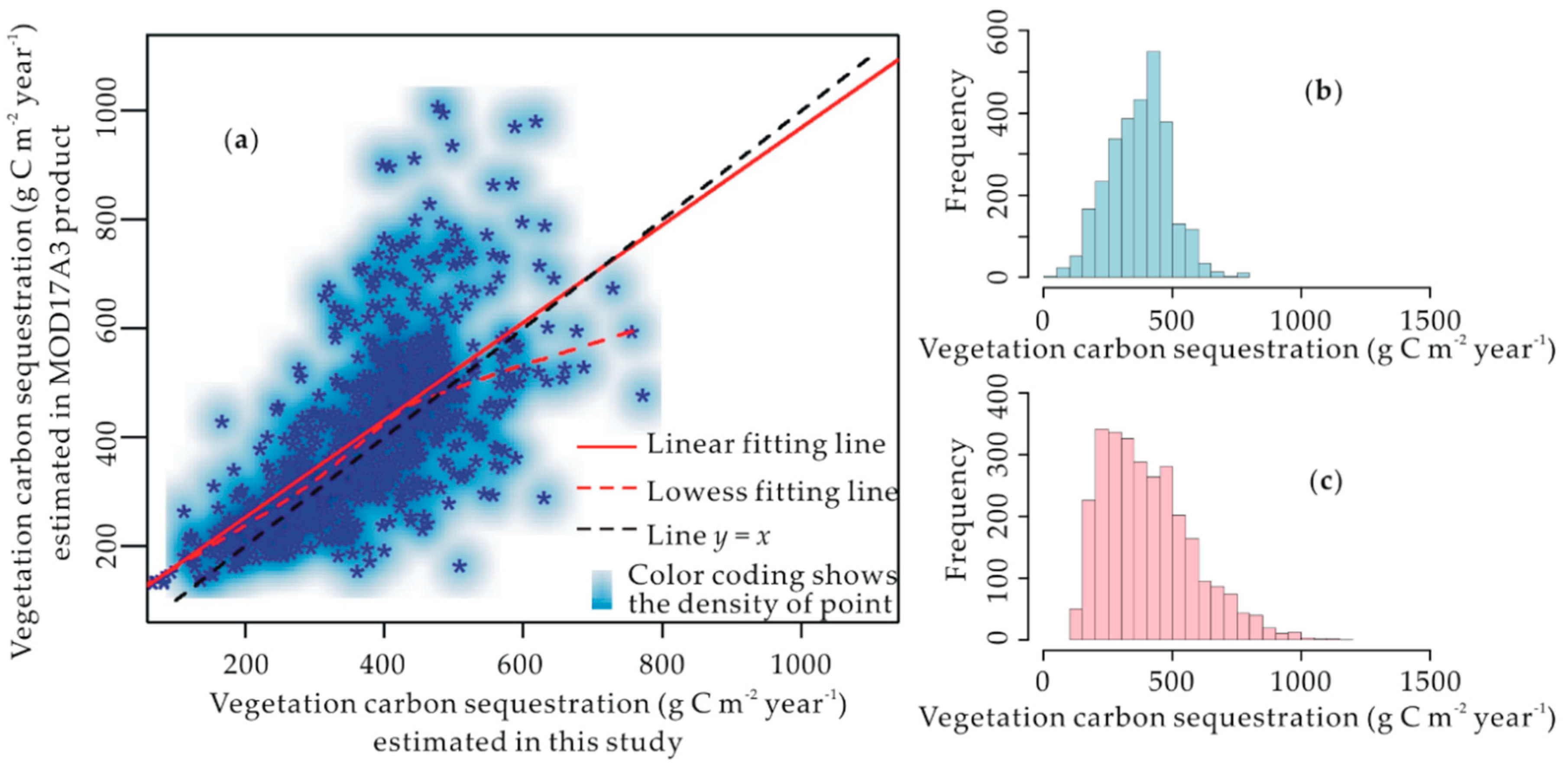
4.1.2. Comparison to the Global Vegetation Production Map

To further evaluate our VI time-series-based method, we compared its estimates with those of the MOD17A3 product (i.e., MOD17A3HGF Version 6 product) [18,19]. The MOD17A3 product is the most widely used global vegetation production map produced by the Numerical Terradynamic Simulation Group/University of Montana by using the radiation use efficiency concept [19]. Figure 9 shows the MOD17A3 estimates in Poyang Lake wetland in 2016. This figure estimated that the vegetation carbon sequestration yielded a mean of 366 g C m−2 year−1 with a standard deviation of 117 g C m−2 year−1. Comparison of the regional average values from the two estimates showed that our estimates were 8.7% higher than the MOD17A3 estimates. Moreover, the standard deviation of our estimates was 31.9% higher than that of the MOD17A3 estimates. This result showed that although the regional average values of the two estimates were similar, the vegetation carbon sequestration along the topographic gradient shows significant variation in the VI time-series-based image (Figure 8), whereas that in the MOD17A3 image is difficult to discern (Figure 9). Additionally, another improvement of our VI time-series-based approach compared to the MOD17A3 product is the much wider spatial applicability in wetlands. Since we noted that the MOD17A3 product depicted 90% of the vegetated area by “no data” in the Poyang Lake wetland. Vegetation in these areas sequestered 6.6 × 10⁵ t carbon in 2016 according to our estimates, accounting for 91.2–91.5% of the total vegetation carbon sequestration of the wetland. Hence, we revealed that the MOD17A3 product dramatically underestimated the total vegetation carbon sequestration of the wetland.
The MOD17A3 map has a resolution of 500 m. After resampling our estimate map to 500 m (by averaging the 250 m pixels in each 500 m pixel), we exhibited a scatter plot to compare the two estimations pixel-by-pixel (Figure 10a). The most high-density region is near the line of y = x, revealing a positive correlation between the estimates of the VI time-series-based model and MOD17A3 product. However, the scatter plot also showed that the MOD17A3 estimates underestimated the vegetation carbon sequestration at midrange and highly productive sites compared with our estimates (as shown by the Lowess fitting line). This phenomenon occurred because the 500 m MOD17A3 image smoothened the high values in the highly productive patches less than 0.25 km2 and surrounded by a mudflat or water surfaces. However, the 250 m map produced by the VI time-series-based method can successfully capture those high values. At the less productive sites, i.e., the wide land–water transition area, the MOD17A3 estimates had no values because the algorithm treated this area as perennial inland fresh water. Actually, the land-water transition area is covered by sparse vegetation and spreads over a larger area than the dense vegetation area in Poyang Lake wetland. Thus, the histogram of the MOD17A3 estimates (Figure 10b) was almost in a normal distribution, whereas that of our estimates (Figure 10c) was deflecting to the left. In summary, the VI time-series-based method could adequately capture both the coverage and fine spatial details of vegetation carbon sequestration in this herbaceous wetland.

4.2. Uncertainty Issues in the VI Time-Series-Based Method

The VI time-series-based method in this study directly estimated the vegetation carbon sequestration of Poyang Lake wetland from the dynamics of biomass carbon stocks. The finding is consistent with the results from other similar herbaceous wetlands and the currently used global map of vegetation production (MOD17A3). However, as mentioned in the Introduction section, the accuracy of its estimates was inevitably affected by two important factors, namely, the time resolution of the VI time series and the accuracy of the biomass carbon stock estimate.
For the time resolution of the VI time series, only VI time series at a sufficient number of intervals can capture all the positive differences in biomass carbon stocks across different times because as plants grow, litter biomass carbon stocks fluctuate frequently. To date, satellite remote sensing has provided abundant high-frequency observations to monitor biomass carbon stocks. However, the VI time series of higher frequency need more ground reference data to retrieve, which are often restricted by the cost and complexity of field works, especially for large wetlands such as the Poyang Lake wetland. Thus, the ideal monitoring frequency of biomass carbon stocks for estimating annual vegetation carbon sequestration should correspond to the growth cycle of vegetation, thus it can capture all the important phenological changes of plants. In our studies, the time interval of the MODIS gridded vegetation indices product MOD13Q1 was 16 days, capturing the general seasonal variations in biomass carbon stocks in this region. We did not try the VI time series of other frequencies, such as the weekly or monthly VI time series. Through the deepened understanding of the details of vegetation phenology changes in the region, an appropriate temporal resolution of the VI time series may be proposed to make the VI time-series-based method more accurate and efficient than it was in this study.
The accuracy of the biomass carbon stock estimate in this study was also limited by many factors. For example, we only used the survey data during September, October, November, and December to simulate the relationship between EVI and the field-observed biomass carbon stocks. The effects of the lack of a sample in other months when field data are unavailable were difficult to avoid. Although we applied strict preprocessing to improve the temporal consistency of the EVI time series to make up for this defect, the accuracy of the biomass carbon stock estimation and the performance of the VI time series-based method could be improved when the survey data become abundant. Moreover, the high density of vegetation in this herbaceous wetland presents a challenge for estimating biomass carbon stocks accurately by remote sensing. In fact, the saturation problem associated with the use of VIs calculated from broad band sensors for biomass carbon estimation in high canopy density vegetation is a well-known phenomenon due to the asymmetrical nature of the relationship between biomass carbon stock and vegetation indices calculated from medium spatial resolution (10–100 m) multispectral sensors by using NIR and red bands [28,34]. Therefore, the model for biomass carbon stock estimation used in this study possibly underestimates the biomass carbon stocks at high observed values. This condition explains why the errors were associated with extremely high biomass carbon stock values in Figure 5 and Figure 6. In recent studies, narrow band vegetation indices from hyperspectral data or WorldView-2 (eight bands including red edge band and 2 m spatial resolution) are increasingly utilized to estimate biomass carbon with high canopy density [35,36]. This condition enables the accurate estimation of the biomass carbon stock at full canopy cover compared with the standard red/NIR indices [34]. However, their applications will greatly increase the cost of the biomass carbon stock estimate in the widespread Poyang Lake wetland. We believe that when this technology is widely used, the costs will be reduced, the reflectance saturation problem will be minimized and the accuracy of biomass carbon stock estimate will improve. Consequently, the VI time-series-based method for annual vegetation carbon sequestration will also improve.
In summary, we revealed that the VI time-series-based method is a practical approach for estimating vegetation carbon sequestration in herbaceous wetlands. Importantly, the method shows great application potential with continuous improvements of frequency of satellite VI images and their ability of retrieving biomass carbon stocks.

5. Conclusions

Estimating the large-scale vegetation carbon sequestration in a herbaceous wetland via the satellite data-driven ecophysiological process models is a great challenge because ecophysiological processes in these environments are complex and changeable. Basing on the cumulative composite of biomass carbon stocks, we described herein a simple but intuitive VI time-series-based approach to estimate the vegetation carbon sequestration in herbaceous wetlands. By applying the VI time-series-based method to a 16 day MODIS EVI product in Poyang Lake wetland in 2016, we reached the following conclusions: (1) The vegetation carbon sequestration of Poyang Lake wetland during 2016 was in the range of 193–1221 g C m−2 year−1 with a mean of 401 g C m−2 year−1 and a standard deviation of 172 g C m−2 year−1. (2) The estimations from our VI time-series-based method were close to those obtained for two other wetlands with a similar latitude to our study area and were consistent with the current global maps of vegetation production (MOD17A3) in this area. Moreover, our VI time-series-based method allows estimates in extensive vegetated areas depicted by ‘no data’ in the MOD17A3 product, which substantially reduced the uncertainty of vegetation carbon sequestration estimate in the Poyang Lake wetland. This study revealed that a high frequency, high-quality VI time series could be used to estimate the carbon sequestration of plants in herbaceous wetlands.

Author Contributions

Conceptualization, G.Y.; data curation, X.D.; formal analysis, X.D.; investigation, R.W.; methodology, D.L.; project administration, G.Y.; resources, R.W.; supervision, G.Y. and D.L.; validation, R.W.; visualization, X.D.; writing—original draft, X.D.; writing—review and editing, D.L. and R.W. All authors have read and agreed to the published version of the manuscript.

Funding

This research was funded by the National Natural Science Foundation of China (Grant No. 41901114), the Fundamental Research Funds for the Central Universities of China (Grant No. B200202024), and the National Postdoctoral Program for Innovative Talent of China (Grant No. BX20190107).

Acknowledgments

We are grateful to Xiaolong Wang, who provided the boundary map of the Poyang Lake wetland used in this study.

Conflicts of Interest

The authors declare no conflict of interest.

References

  1. Erickson, J.E.; Peresta, G.; Montovan, K.J.; Drake, B.G. Direct and indirect effects of elevated atmospheric CO2 on net ecosystem production in a Chesapeake Bay tidal wetland. Glob. Chang. Biol. 2013, 19, 3368–3378. [Google Scholar] [CrossRef]
  2. Strack, M. Peatlands and Climate Change. Ph.D. Thesis, University of Calgary, Alberta, AB, Canada, 2008. [Google Scholar]
  3. WMO Greenhouse Gas Bulletin. Available online: https://public.wmo.int/en/resources/library/wmo-greenhouse-gas-bulletin (accessed on 3 January 2018).
  4. Joos, F.; Spahni, R. Rates of change in natural and anthropogenic radiative forcing over the past 20,000 years. Proc. Natl. Acad. Sci. USA 2008, 105, 1425–1430. [Google Scholar] [CrossRef] [PubMed] [Green Version]
  5. Nahlik, A.M.; Fennessy, M.S. Carbon storage in US wetlands. Nat. Commun. 2016, 7, 13835. [Google Scholar] [CrossRef] [Green Version]
  6. Pierfelice, K.N.; Lockaby, B.G.; Krauss, K.W.; Conner, W.H.; Noe, G.B.; Ricker, M.C. Salinity Influences on Aboveground and Belowground Net Primary Productivity in Tidal Wetlands. J. Hydrol. Eng. 2015, 22, D5015002. [Google Scholar] [CrossRef]
  7. Peregon, A.; Maksyutov, S.; Kosykh, N.P.; Mironycheva-Tokareva, N.P. Map-based inventory of wetland biomass and net primary production in western Siberia. J. Geophys. Res. 2008, 113, 1–12. [Google Scholar] [CrossRef]
  8. Caplan, J.S.; Hager, R.N.; Megonigal, J.P.; Mozdzer, T.J. Global change accelerates carbon assimilation by a wetland ecosystem engineer. Environ. Res. Lett. 2015, 10, 115006. [Google Scholar] [CrossRef]
  9. Han, G.; Yang, L.Q.; Yu, J.B.; Wang, G.M.; Mao, P.L.; Gao, Y.J. Environmental controls on net ecosystem CO2 exchange over a reed (Phragmites australis) wetland in the Yellow River Delta, China. Estuar. Coast 2012, 36, 401–413. [Google Scholar] [CrossRef]
  10. Zheng, Y.M.; Niu, Z.G.; Gong, P.; Dai, Y.J.; Shangguan, W. Preliminary estimation of the organic carbon pool in China’s wetlands. Chin. Sci. Bull. 2012, 58, 662–670. [Google Scholar] [CrossRef] [Green Version]
  11. Xu, X.B.; Yang, G.S.; Tan, Y.; Tang, X.G.; Jiang, H.; Sun, X.X.; Zhang, Q.L.; Li, H.P. Impacts of land use changes on net ecosystem production in the Taihu Lake Basin of China from 1985 to 2010. J. Geophys. Res.-Biogeosci. 2017, 122, 690–707. [Google Scholar] [CrossRef]
  12. Peregon, A.; Kosykh, N.P.; Mironycheva-Tokareva, N.P.; Ciais, P.; Yamagata, Y. Estimation of Biomass and Net Primary Production (NPP) in West Siberian Boreal Ecosystems: In Situ and Remote Sensing Methods. In Novel Methods for Monitoring and Managing Land and Water Resources in Siberia; Mueller, L., Sheudshen, A.K., Eulenstein, F., Eds.; Springer International Publishing: Heidelberg, Germany, 2016; pp. 233–252. [Google Scholar]
  13. Kayranli, B.; Scholz, M.; Mustafa, A.; Hedmark, A. Carbon Storage and Fluxes within Freshwater Wetlands: A Critical Review. Wetlands 2009, 30, 111–124. [Google Scholar] [CrossRef]
  14. Costa, W.; Tortarolo, G.M.; Harper, A.; Sitch, S. Capacity for Carbon Sequestration and Climate Change Mitigation in Different Ecologically-Distinct Zones of Sri Lanka. In Session VIII–Climate Change, Land Degradation and Disaster Management. Proceedings of International Forestry and Environment Symposium; University of Sri Jayewardenepura: Nugegoda, Sri Lanka, 2015. [Google Scholar]
  15. Field, C.B.; Randerson, J.T.; Malmstrom, C.M. Global net primary production: Combining ecology and remote sensing. Remote Sens. Env. 1995, 281, 237–240. [Google Scholar] [CrossRef] [Green Version]
  16. Prince, S.; Goward, S. Global primary production: A remote sensing approach. J. Biogeogr. 1995, 22, 815–835. [Google Scholar] [CrossRef]
  17. Turner, D.P.; Ritts, W.D.; Cohen, W.B.; Gower, S.T.; Zhao, M.; Running, S.W.; Wofsy, S.C.; Urbansky, S.; Dunn, A.L.; Munger, J.W. Scaling gross primary production (GPP) over boreal and deciduous forest landscapes in support of MODIS GPP product validation. Remote Sens. Environ. 2003, 88, 256–270. [Google Scholar] [CrossRef] [Green Version]
  18. Running, S.W.; Hunt, E.R. Generalization of a forest ecosystem process model for other biomes, BIOME-BGC, and an application for global-scale models. In Scaling Physiological Processes: Leaf to Globe, 1st ed.; Ehleringer, J.R., Field, C.B., Eds.; Academic Press: San Diego, CA, USA, 1993; pp. 141–158. [Google Scholar] [CrossRef]
  19. Running, S.W.; Nemani, R.R.; Heinsch, F.A.; Zhao, M.; Reeves, M.; Hashimoto, H. A continuous satellite-derived measure of global terrestrial primary production. Bioscience 2004, 54, 547–560. [Google Scholar] [CrossRef]
  20. Heinsch, F.A.; Zhao, M.S.; Running, S.W.; Kimball, J.S.; Nemani, R.R.; Davis, K.J.; Bolstad, P.V.; Cook, B.D.; Desai, A.R.; Ricciuto, D.M.; et al. Evaluation of remote sensing based terrestrial productivity from MODIS using regional tower eddy flux network observations. IEEE Trans. Geosci. Remote Sens. 2006, 44, 1908–1925. [Google Scholar] [CrossRef] [Green Version]
  21. Sims, D.A.; Rahman, A.F.; Cordova, V.D.; El-Masri, B.Z.; Baldocchi, D.D.; Flanagan, L.B.; Goldstein, A.H.; Hollinger, D.Y.; Misson, L.; Monson, R.K.; et al. On the use of MODIS EVI to assess gross primary productivity of North American ecosystems. J. Geophys. Res. 2006, 111, G04015. [Google Scholar] [CrossRef] [Green Version]
  22. Rahman, A.F.; Sims, D.A.; Cordova, V.D.; El-Masri, B.Z. Potential of MODIS EVI and surface temperature for directly estimating per-pixel ecosystem C fluxes. Geophys. Res. Lett. 2005, 32, L19404. [Google Scholar] [CrossRef] [Green Version]
  23. Sjöström, M.; Ardö, J.; Arneth, A.; Boulain, N.; Cappelaere, B.; Eklundh, L.; Grandcourt, A.; Kutsch, W.L.; Merbold, L.; Nouvellon, Y.; et al. Exploring the potential of MODIS EVI for modeling gross primary production across African ecosystems. Remote Sens. Environ. 2011, 115, 1081–1089. [Google Scholar] [CrossRef]
  24. Costa, M.; Evans, T.; Silva, T.S.F. Remote Sensing of Wetland Types: Subtropical Wetlands of Southern Hemisphere. In The Wetland Book; Finlayson, C.M., Everard, M., Irvine, K., Mclnnes, R.J., Middleton, B.A., van Dam, A.A., Davidson, N.C., Eds.; Springer: South Holland, The Netherlands, 2018; Chapter 307; pp. 1673–1678. [Google Scholar] [CrossRef]
  25. Hoekman, D. Remote Sensing of Wetland Types: Peat Swamps. In The Wetland Book; Finlayson, C.M., Everard, M., Irvine, K., Mclnnes, R.J., Middleton, B.A., van Dam, A.A., Davidson, N.C., Eds.; Springer: South Holland, The Netherlands, 2018; Chapter 306; pp. 1649–1657. [Google Scholar] [CrossRef]
  26. Dai, X.; Wan, R.R.; Yang, G.S.; Wang, X.L.; Xu, L.G. Responses of wetland vegetation in Poyang Lake, China to water-level fluctuation. Hydrobiologia 2016, 773, 35–37. [Google Scholar] [CrossRef]
  27. Dai, X.; Wan, R.R.; Yang, G.S.; Wang, X.L.; Xu, L.G.; Li, Y.Y.; Li, B. Impact of seasonal water-level fluctuations on autumn vegetation in Poyang Lake wetland, China. Front. Earth Sci. 2019, 13, 398–409. [Google Scholar] [CrossRef]
  28. Mutanga, O.; Adam, E.; Cho, M.A. High density biomass estimation for wetland vegetation using WorldView-2 imagery and random forest regression algorithm. Int. J. Appl. Earth Obs. 2012, 18, 399–406. [Google Scholar] [CrossRef]
  29. Li, X.; Gar-On Yeh, A.; Wang, S.; Liu, K.; Liu, X.; Qian, J.; Chen, X. Regression and analytical models for estimating mangrove wetland biomass in South China using Radarsat images. Int. J. Remote Sens. 2007, 28, 5567–5582. [Google Scholar] [CrossRef]
  30. Rouse, J.W.; Haas, R.H.; Schell, J.A.; Deering, D.W. Monitoring vegetation systems in the Great Plains with ERTS. Nasa Spec. Publ. 1973, 351, 301–317. [Google Scholar]
  31. Huete, A.R. A soil-adjusted vegetation index (SAVI). Remote Sens. Environ. 1988, 25, 295–309. [Google Scholar] [CrossRef]
  32. Qi, J.; Chehbouni, A.; Huete, A.R.; Kerr, Y.H.; Sorooshian, S. A modified soil adjusted vegetation index. Remote Sens. Environ. 1994, 48, 119–126. [Google Scholar] [CrossRef]
  33. Kaufman, Y.J.; Tanré, D. Atmospherically resistant vegetation index (ARVI) for EOS-MODIS. IEEE Trans. Geosci. Remote Sens. 1992, 30, 261–270. [Google Scholar] [CrossRef]
  34. Mutanga, O.; Skidmore, A.K. Narrow band vegetation indices overcome the saturation problem in biomass estimation. Int. J. Remote Sens. 2004, 25, 3999–4014. [Google Scholar] [CrossRef]
  35. Thenkabail, P.S.; Smith, R.B.; Pauw, E.D. Hyperspectral vegetation indices and their relationships with agricultural crop characteristics. Remote Sens. Environ. 2000, 71, 158–182. [Google Scholar] [CrossRef]
  36. Lu, D. The potential and challenge of remote sensing–based biomass estimation. Int. J. Remote Sens. 2006, 27, 1297–1328. [Google Scholar] [CrossRef]
  37. Gao, F.; Hilker, T.; Zhu, X.; Anderson, M.; Masek, J.; Wang, P.; Yang, Y. Fusing Landsat and MODIS Data for Vegetation Monitoring. IEEE Geosci. Remote Sens. Mag. 2015, 3, 47–60. [Google Scholar] [CrossRef]
  38. Kwan, C.; Budavari, B.; Gao, F.; Zhu, X. A Hybrid Color Mapping Approach to Fusing MODIS and Landsat Images for Forward Prediction. Remote Sens. 2018, 10, 520. [Google Scholar] [CrossRef] [Green Version]
  39. Huete, A.; Didan, K.; Miura, T.; Rodriguez, E.P.; Gao, X.; Ferreira, L.G. Overview of the radiometric and biophysical performance of the MODIS vegetation indices. Remote Sens. Environ. 2002, 83, 195–213. [Google Scholar] [CrossRef]
  40. Hird, J.N.; McDermid, G.J. Noise reduction of NDVI time series: An empirical comparison of selected techniques. Remote Sens. Environ. 2009, 113, 248–258. [Google Scholar] [CrossRef]
  41. Chen, J.; Jönsson, P.; Tamura, M.; Gu, Z.H.; Matsushita, B.; Eklundh, L. A simple method for reconstructing a high-quality NDVI time-series data set based on the Savitzky-Golay filter. Remote Sens. Environ. 2004, 91, 332–344. [Google Scholar] [CrossRef]
  42. Jönsson, P.; Eklundh, L. Seasonality extraction by function fitting to time-series of satellite sensor data. IEEE Trans. Geosci. Remote Sens. 2002, 40, 1824–1832. [Google Scholar] [CrossRef]
  43. Jönsson, P.; Eklundh, L. TIMESAT—a program for analyzing time-series of satellite sensor data. Comput. Geosci. 2004, 30, 833–845. [Google Scholar] [CrossRef] [Green Version]
  44. Viovy, N.; Arino, O.; Belward, A.S. The Best Index Slope Extraction (BISE): A method for reducing noise in NDVI time-series. Int. J. Remote Sens. 1992, 13, 1585–1590. [Google Scholar] [CrossRef]
  45. Cihlar, J. Identification of contaminated pixels in AVHRR composite images for studies of land biosphere. Remote Sens. Environ. 1996, 56, 149–153. [Google Scholar] [CrossRef]
  46. Sellers, P.J.; Tucker, C.J.; Collatz, G.J.; Los, S.O.; Justice, C.O.; Dazlich, D.A.; Randall, D.A. A global 1 by 1 NDVI data set for climate studies: Part II. The generation of global fields of terrestrial biophysical parameters from the NDVI. Int. J. Remote Sens. 1994, 15, 3519–3545. [Google Scholar] [CrossRef]
  47. Lunetta, R.S.; Knight, J.F.; Ediriwickrema, J.; Lyon, J.G.; Worthy, L.D. Land-cover change detection using multi-temporal MODIS NDVI data. Remote Sens. Environ. 2006, 105, 142–154. [Google Scholar] [CrossRef]
  48. Zhang, X.Y.; Friedl, M.A.; Schaaf, C.B.; Strahler, A.H.; Hodges, J.C.F.; Gao, F.; Reed, B.C.; Huete, A. Monitoring vegetation phenology using MODIS. Remote Sens. Environ. 2003, 84, 471–475. [Google Scholar] [CrossRef]
  49. Lovell, J.L.; Graetz, R.D. Filtering pathfinder AVHRR land NDVI data for Australia. Int. J. Remote Sens. 2001, 22, 2649–2654. [Google Scholar] [CrossRef]
  50. Dai, X.; Wan, R.R.; Yang, G.S. Non-stationary water-level fluctuation in China’s Poyang Lake and its interactions with Yangtze River. J. Geogr. Sci. 2015, 25, 274–288. [Google Scholar] [CrossRef] [Green Version]
  51. Shankman, D.; Keim, B.D.; Song, J. Flood frequency in China’s Poyang Lake region: Trends and teleconnections. Int. J. Clim. 2006, 26, 1255–1266. [Google Scholar] [CrossRef] [Green Version]
  52. Sang, H.; Zhang, J.; Lin, H.; Zhai, L. Multi-Polarization ASAR Backscattering from Herbaceous Wetlands in Poyang Lake Region, China. Remote Sens. 2014, 6, 4621–4646. [Google Scholar] [CrossRef] [Green Version]
  53. Liu, Q.; Yan, B.Y.; Ge, G.; Tan, H.R. Theory and Practice of Ecological Restoration for Poyang Lake Wetland, 1st ed.; Science Press: Beijing, China, 2012; pp. 166–199, (In Chinese with English Abstract). [Google Scholar]
  54. Dai, X. Effects of Hydrological Conditions on Vegetation Carbon Sequestration of Poyang Lake Wetland. Ph.D. Thesis, University of Chinese Academy of Sciences, Beijing, China, 2018. (In Chinese with English Abstract). [Google Scholar]
  55. Cleveland, R.B.; Cleveland, W.S.; McRae, J.E.; Terpenning, I. STL: A Seasonal-Trend Decomposition Procedure Based on Loess. J. Off. Stat. 1990, 6, 3–73. [Google Scholar]
  56. Savitzky, A.; Golay, M.J.E. Smoothing and differentiation of data by simplified least squares procedures. Anal. Chem. 1964, 36, 1627–1639. [Google Scholar] [CrossRef]
  57. Wu, G.P.; Ye, C.; Liu, Y.B. Spatial distribution of wetland vegetation biomass in the Poyang Lake National Nature Reserve, China. Acta Ecol. Sin. 2015, 35, 361–369. [Google Scholar] [CrossRef] [Green Version]
  58. Buffam, I.; Turner, M.G.; Desai, A.R.; Hanson, P.C.; Rusak, J.A.; Lottig, N.R.; Stanley, E.H.; Carpenter, S.R. Integrating aquatic and terrestrial components to construct a complete carbon budget for a north temperate lake district. Glob. Chang. Biol. 2011, 17, 1193–1211. [Google Scholar] [CrossRef]
  59. Garnier, E.; Laurent, G. Leaf anatomy, specific mass and water content in congeneric annual and perennial grass species. New Phytol. 1994, 128, 725–736. [Google Scholar] [CrossRef]
  60. Mei, X.Y.; Zhang, X.F. Carbon storage and fixation function of Scirpusmariqueter in Changjiang river estuary: A case Study of Chongming Dongtan wetland. J. Agro-Environ. Sci. 2007, 26, 360–363, (In Chinese with English Abstract). [Google Scholar]
  61. Mao, Z.G.; Wang, G.X.; Liu, J.E.; Ren, L.J. Influence of salt marsh vegetation on spatial distribution of soil carbon and nitrogen in Yancheng coastal wetland. Chin. J. Appl. Ecol. 2009, 20, 293–297, (In Chinese with English Abstract). [Google Scholar]
  62. Belyea, L.R.; Warner, B.G. Temporal scale and the accumulation of peat in a Sphagnum bog, Canadian. J. Bot. 2011, 74, 366–377. [Google Scholar]
Figure 1. Poyang Lake wetland. (a) Location of the Poyang Lake wetland; (b) land cover map of the Poyang Lake wetland in 2016 interpreted by Dai [54]; and (c) aerial view of a typical coastline with Phragmites community and Carex community changing with elevation from high to low on the marsh areas.
Remotesensing 12 03000 g001
Figure 2. Example showing the quality of the processed enhanced vegetation index (EVI) time series (EVI data from the test pixel at 29°10′0″ N, 116°0′0″ E).
Remotesensing 12 03000 g002
Figure 3. Sampling locations in field survey. (a) Location of the typical inflow river delta and its 14 samples; (b) location of the littoral land of the main lake and its 41 samples; (c) location of the typical sublakes and its 24 samples; and (d) location of the typical small islands and its 7 samples (the background image is a false color composition of the Landsat 8 image with the band 5, band 4, and band 3 to red, green, and blue, respectively).
Remotesensing 12 03000 g003
Figure 4. Raw and processed EVI time series by using different methods at randomly selected test pixels.
Remotesensing 12 03000 g004
Figure 5. Relationship between EVI (x) and biomass carbon stock (y) in Poyang Lake wetland. (a) The relationship fitted by the power law model; (b) the relationship fitted by the exponential model; (c) the relationship fitted by the linear regression model; and (d) the relationship fitted by the polynomial model.
Remotesensing 12 03000 g005
Figure 6. Observed biomass carbon stocks vs. predicted biomass carbon stocks by the quadratic polynomial regression model: (a) training results and (b,c) testing results.
Remotesensing 12 03000 g006
Figure 7. Inner-annual variations of biomass carbon stocks in Poyang Lake wetland in 2016.
Remotesensing 12 03000 g007
Figure 8. Vegetation carbon sequestration of Poyang Lake wetland in 2016 estimated in this study.
Remotesensing 12 03000 g008
Figure 9. Vegetation carbon sequestration of Poyang Lake wetland in 2016 estimated by MOD17A3.
Remotesensing 12 03000 g009
Figure 10. Scatter plot of vegetation carbon sequestration estimated from MOD17A3 and the vegetation index (VI) time series-based method (a); comparison of histograms between the estimates of MOD17A3 (b); and the VI time-series-based method (c).
Remotesensing 12 03000 g010
Table 1. Estimates of vegetation carbon sequestration in previous studies.
SpeciesCarbon Sequestration
(g C m−2 yr−1)
RegionReference
Mixtures of Phragmites spp. and Carex spp.401 ± 172
(regional average)
Poyang Lake wetlandEVI time series-based method
Phragmites community669 ± 134
(regional average)
Carex community259 ± 140
(regional average)
Phragmites community745 ± 12
(sample-site value)
Carex community495 ± 71
(sample-site value)
Scirpus mariqueter510
(sample-site value)
East Chongming wetlandMei and Zhang 2007 [60]
Herba suaedae504
(sample-site value)
Yancheng coastal wetlandMao et al. 2009 [61]
Scirpus triqueter1330
(sample-site value)
Phragmites spp.1290
(sample-site value)

