Article

RGB Image-Derived Indicators for Spatial Assessment of the Impact of Broadleaf Weeds on Wheat Biomass

by
Christelle Gée
1,* and
Emmanuel Denimal
2
1
Agroécologie, AgroSup Dijon, INRAE, Univ. Bourgogne, Univ. Bourgogne Franche-Comté, F-21000 Dijon, France
2
AgroSup Dijon, Service Système d’Information Appui à la Recherche et Enseignement Supérieur, 26 Bd Dr Petitjean, 21000 Dijon, France
*
Author to whom correspondence should be addressed.
Remote Sens. 2020, 12(18), 2982; https://doi.org/10.3390/rs12182982
Submission received: 23 June 2020 / Revised: 3 September 2020 / Accepted: 10 September 2020 / Published: 14 September 2020
(This article belongs to the Section Remote Sensing in Agriculture and Vegetation)

Abstract

:
In precision agriculture, the development of proximal imaging systems embedded in autonomous vehicles allows to explore new weed management strategies for site-specific plant application. Accurate monitoring of weeds while controlling wheat growth requires indirect measurements of leaf area index (LAI) and above-ground dry matter biomass (BM) at early growth stages. This article explores the potential of RGB images to assess crop-weed competition in a wheat (Triticum aestivum L.) crop by generating two new indicators, the weed pressure (WP) and the local wheat biomass production ( δ BMc ). The fractional vegetation cover (FVC) of the crop and the weeds was automatically determined from the images with a SVM-RBF classifier, using bag of visual word vectors as inputs. It is based on a new vegetation index called MetaIndex, defined as a vote of six indices widely used in the literature. Beyond a simple map of weed infestation, the map of WP describes the crop-weed competition. The map of δBMc, meanwhile, evaluates the local wheat above-ground biomass production and informs us about a potential stress. It is generated from the wheat FVC because it is highly correlated with LAI (r2 = 0.99) and BM (r2 = 0.93) obtained by destructive methods. By combining these two indicators, we aim at determining whether the origin of the wheat stress is due to weeds or not. This approach opens up new perspectives for the monitoring of weeds and the monitoring of their competition during crop growth with non-destructive and proximal sensing technologies in the early stages of development.

Graphical Abstract

1. Introduction

The emergence of proximal sensing technologies in precision agriculture provides new opportunities to drastically reduce chemical herbicides from site-specific weed management (SSWM) while maintaining production yield, quality, and commercial value [1,2,3]. Although weed management in field crops is a long story [4,5], it is still topical [6,7,8]. The development of affordable and easy to use unmanned aerial vehicles (UAV) allows accurate weed monitoring thanks to high resolution images [9,10,11]. Imaging systems are mostly based on multi or hyperspectral optical sensors. They require complex image processing algorithms to discriminate between crops and weeds and to generate weed maps [11,12,13]. The first step consists of extracting vegetation pixels in the image. The remote sensing community developed spectral indices to quantify greenness in a multispectral image [14,15,16]. The segmentation is generally performed using vegetation indices built as a combination of spectral bands. Their choice depends on the application: for RGB images, the most common is the excess green index (ExG or 2g-r-b index) proposed by Woebbecke et al. [14]. When the near infrared band is available, the normalized difference vegetation index (NDVI) is a classic [17]. Tang et al. [18] highlighted the pros and cons of color indices for plant-background segmentation. With aerial images captured from an UAV, Torres-Sanchez et al. [15] demonstrated that, among different vegetation indexes, the ExG and VEG indices performed best in vegetation fraction mapping. Our study focuses on the MetaIndex, a new vegetation index that takes advantage of six common indices.
Several image classifiers based on machine learning have been successfully applied to classify plants and to identify weed species [19,20,21,22]. The recent development of high resolution UAV imagery [20,23,24,25] allowed fast and accurate crop weed recognition. Depending on the crop (wheat, sunflower, maize…) and the weed, these algorithms lead to 75−95% classification accuracy. Pérez–Ortiz et al. [25] compared several classification algorithms on multispectral images (six wavebands) acquired by UAV over sunflower at three flight altitudes. They demonstrated that, regardless of the method, the higher the resolution of the images, the better the results. Peña et al. [9] applied an object-based image analysis (OBIA) to generate weed infestation maps from UAV imagery. They could discriminate three categories of weed coverage in maize crops with 86% overall accuracy. Using convolutional neural network (CNN), Huang et al. [12] were able to differentiate rice from unspecified weeds, with 97% accuracy. Bah et al. [26] developed a new automatic learning method also based on CNN for weed detection in UAV images, with an unsupervised training dataset. Support vector machine (SVM) are powerful supervised learning classifiers to discriminate vegetation in a complex case, e.g., overlapping leaves. Pérez–Ortiz et al. [20] used SVM to classify crop/weed from RGB images in sunflower and maize fields. Suh et al. [27] compared different machine learning classifiers to differentiate sugar beet from volunteer potato plants, concluding that SVM was more efficient than random forest or neural networks. Pflanz et al. [8] could discriminate between wheat and weeds with 98% accuracy and differentiate various weed species with 87% accuracy. Thus, weed mapping is a major issue to provide decision-making support for variable rate spraying application [28,29]. However, due to the reduction of chemical inputs and to climate change, particular attention should be given to a regular and precise monitoring of crop growth [30,31]. Indeed, the emergence of crop stressors can negatively impact on plant development and ultimately crop productivity [31,32]. Therefore, maintaining weed flora below a nuisance threshold by non-destructive measurements is a major challenge for spatio-temporal crop and weed monitoring. Early monitoring of crop- weed competition is essential to develop new control strategies of weed emergence and anticipate their management. Competition indicators are generally based on density measurements or visual plant recognition, which are time-consuming and labor-intensive for farming practices. Other parameters such as dry matter biomass (BM) and leaf area index (LAI) can be measured by destructive methods, also time-consuming [33,34,35]. Recent research revealed that the BMw/BMc ratio could express crop-weed competition [36]. Non-destructive methods based on optical imaging devices may be powerful to study weed competition and monitor wheat growth, especially at early growth stages. Several articles [37,38,39] report indirect estimation of BM and LAI using vegetation indices and spectral analysis [40,41,42,43] by determining the proportion of ground occupied by vegetation (i.e., vegetation cover, vegetation fraction or fractional vegetation cover, fraction of green cover). Thus, digital image approaches became an alternative solution to infer plant biomass [39,44], especially at early growth stages. They allow monitoring plants over time for crop protection management.
This article aims to evaluate the origin of wheat stress while looking at weed infestation using RGB images. The first part describes the acquisition of data on three different dates. Then we present the image-processing algorithm for crop/weed discrimination and introduce a new vegetation index called MetaIndex. The calibration between destructive (LAI and BM) and non-destructive (FVC) measurements deduced from an in-field image acquisition system is investigated. In a second part, two new non-destructive indicators are generated to evaluate the weed pressure (WP) and the local evaluation of wheat biomass production on wheat growth (δBMc) informing about a potential stress.

2. Materials and Methods

2.1. Study Site and Data Acquisition

The study site is located in Dijon, Burgundy, France (47°18′32″ N, 5°04′0.165″ E). The experiment was conducted in 2018 during the early stages of winter wheat (Triticum aestivum L.) growth, from the 3-leaf stage to tillering on three sampling dates: 23 March, 6 April, and 12 April 2018. No nitrogen nor weed management was applied. The weed flora is composed of annual dicots such as Polygonum aviculare L. (EPPO code: POLAV), Fallopia convolvulus L. (POLCO), Capsella bursa-pastoris (L.) Medicus (CAPBP) and perennial dicots such as Convolvulus arvensis L. (CONAR). These plants are not representative of wheat crops. The emergence of unspecific weeds reveals the history of the plot and the agricultural practices (previous crop and tillage). The Apache cultivar was sown on 12 November 2017 on a chalky-clay deep soil with a density of 345 g.m−2. The plot (1.2 m × 15 m = 18 m2) was composed of seven crop rows separated by a distance of 0.15 m (Figure 1a). It was divided into three subplots associated to each sampling date. Destructive measurements, sample collection (wheat and weeds), and RGB image acquisition were performed in each quadrat (S = 0.45 m × 0.76 m = 0.342 m2). There were three replicates per date.
The destructive measurements served as a reference. The aerial parts of the wheat and the weeds were collected separately and were packed into paper bags. We measure the leaf area index (LAI expressed in m2.m−2) using a planimeter. Then, for each sampling date, the above-ground dry matter biomass (BM, g.m−2) was determined by weighing plants, after being oven dried at 80 °C for 48 h.
In parallel, we built a movable sensing platform made of PVC pipes, on which a Canon EOS 450D (Canon Inc., Tokyo, Japan) commercial digital camera was mounted at a height of 1 m (Figure 1b). Capturing vertical images allows comparing the results with LAI at early growth stages. The main parameters of the camera are described in Table A1 (Appendix A). The camera shutter was controlled remotely. Each experiment was conducted in clear weather under stable light conditions. The exposure time and shutter speed were optimized for the light conditions. The RGB images have a spatial resolution of 0.2 mm/pixel. Images were acquired before sampling the plants. For each measure, two images are shot: one before plant sampling and containing both the wheat and weed populations, and another after the wheat plants were removed, therefore, containing only weeds. Outside the sampling and measurement areas, six images of wheat were taken this way. These images labelled “weeds” and “wheat” will be used, after being transformed into thousands of thumbnail images to feed the classifier during the training phase. In total, 18 images were recorded at several plant growth stages listed in Table 1.
On the first date only, the whole surface of the plot was imaged. As for a UAV platform, we built an orthomosaic photo of the entire plot with a ~60% overlap between successive images and a ~40% overlap between passes. We used Image Composite Editor (Version 2.0.3.0, 2015, Microsoft Corporation, Redmond, WA, USA), an image stitcher software, to create a panoramic image.

2.2. Image Processing

Figure 2 illustrates the flowchart of the methodology used to generate output maps to assess crop-weed competition. After the data collection (step A), the image processing (step B) determines the fractional vegetation cover (FVC) of both the wheat (FVCc) and the weeds (FVCw). It is defined as the ratio of the number of pixels of vegetation (crop vs. weeds) to the total number of pixels in the image. Then, a correlation is established between FVCc and BMc to map wheat biomass. In step C, information about the effect of weed on wheat crop is provided by two non-destructive image-derived indicators: the weed pressure (WP) and the wheat biomass production, δBMc.
The image processing (step B) pipeline can be summarized in four steps: (1) segmentation of the initial RGB image to create a vegetation image from a MetaIndex; (2) feature extraction from bag of visual word (BoVW) descriptors using superpixels of vegetation; and (3) supervised classification from support vector machine (SVM) to discriminate crop from weeds.
All the image pre-processing and processing algorithms were implemented in Matlab (Version 2016b, The Mathworks, Natick, MA, USA).
Greenness identification from MetaIndex (step B-1). We propose the new vegetation index called MetaIndex, which combines the advantages of six vegetation indices (Table 2) commonly used in the literature and recently reported in Baniaich et al. [45], Meyer et al. [16], Guo et al. [46], and Yang et al. [47]. It consists in assigning a pixel to a class (vegetation or other) by a majority vote performed on four indices over the six listed in Table 2. This method is completed by a geodesic segmentation to refine the results and obtain a B&W vegetation image also called B&W vegetation mask (white pixel for the vegetation, black for the background).
Feature extraction (step B-2). The input data of the two-class SVM-RBF classifier is not the RGB image but a vector of main features specific to each class (crop vs. weed). Extraction of these features is quite complex and requires several image-processing steps. To reduce computation time, superpixels (128 × 128 px) are then created with the SLIC (Simple Linear Iterative Clustering) algorithm commonly used in the literature [26]. Combining a RGB image with its vegetation mask, only superpixels of vegetation are kept in the thumbnail images. We used the labelled ones to create the crop and weed training dataset (Figure 3). The SURF (speeded-up robust features) descriptor algorithm [51] allows extracting features (~1000) from these images. Thousands of variables are then extracted in each stand to construct a 500-dimensional BoVW vector, containing the most influential features (~500) owing the Bag of Visual World method [27,52,53]. This approach is very popular in agriculture to discriminate between crop and weeds [8,27,51]. With the labelled image database, the BoVW vector of each thumbnail is associated to a class, wheat or weeds. From this technique, we increase easily the number of labelled images of the training dataset.
Supervised classification and evaluation (step B-3). The classifier learns how to distinguish the crop from the weed flora (training phase). It is based on a support vector machine (SVM) algorithm [54] with a radial basis function (Gaussian type). Among all supervised techniques used for crop/weed discrimination, SVM-RBF is one of the most powerful classification algorithms based on machine learning [8,11,21,23,25,55].
The learning dataset is made of 7860 thumbnails labelled into two classes: crop and weed. The classifier algorithm is calibrated from the learning set divided into a training set and a validation set. Labelled thumbnail images were randomly selected from the learning set with 85% for training and 15% for validation. Once the classification algorithm is validated, we test it with a new RGB image. Then a new BoVW vector is produced in relation to the codebook, and using the calibrated image classifier, the new BoVW vector is labelled as crop or weed. Finally we can build crop and weed maps, and calculate the respective fractional vegetation cover (FVC), FVCc and FVCw (Figure 2).
The calculation of specific statistical metrics derived from the confusion matrix [56] allows assessing the SVM-learning algorithm. Three metrics were computed for performance evaluation: Recall (Equation (1)) reflects the ability to reveal the needed information; Precision (Equation (2)) indicates the correctness of the detected results; F-score (Equation (3)) indicates the balance between Precision and Recall.
Recall = TP TP + FN
Precision = TP TP + FP
F score = 2 × Recall × Precision Precision + Recall
with TP being the number of true positives, FP and FN are the number of false positives and false negatives, respectively [8,56].

2.3. Two Non-Destructive Indicators for a Crop-Weed Competition

Accurate monitoring of weeds while controlling wheat growth requires indirect measurements of leaf area index (LAI) and dry matter biomass (BM) at early wheat growth stage. Therefore, it is necessary to measure LAI and BM destructively to correlate them to FVCc. We developed two indicators deduced from the image. The weed pressure (WP) characterizes the relationship between crop and weed. For their growth, plants are in direct competition for water, nutrients and for light, main parameter at the end of winter. However, this indicator alone is not sufficient to conclude on the negative weed impact on wheat crop. The second indicator is a local above-ground biomass production, δBMc. It provides information about stress but not about its cause. To check whether the stress originates from weeds or not, it has to be compared with the WP.
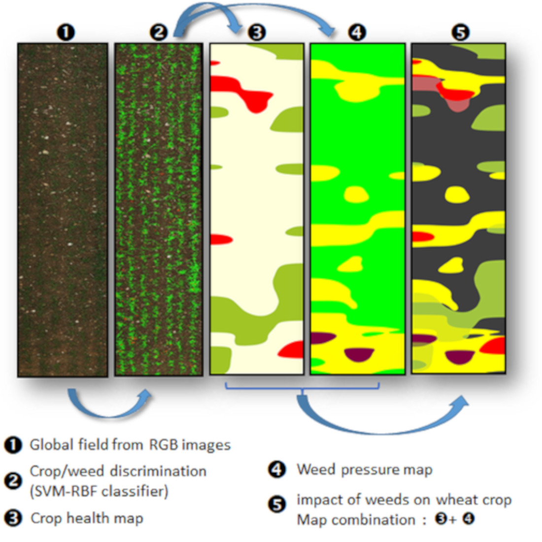
  • The weed pressure (WP) is expressed as a percentage and defined as
    WP   =   100   ×   FVC w   /   FVC c
with FVCw ,   the fractional weed vegetation cover, and FVCc ,   the fractional wheat vegetation cover. It provides information on the resource competition between the crop and the weeds: light, nutrients, and nitrogen. WP can be viewed as a substitute to the BMw/BMc ratio, which results from a destructive approach until the tillering stage by late winter.
  • Evaluation of the local wheat above-ground biomass production: δBMc
The objective of this second indicator is to observe locally the wheat biomass ( δ BM o b s ) and to compare it to a reference value ( BM r e f ) from the image parameter, FVCc . It is defined as
δ BMc   =   BM r e f   BM o b s
with BM r e f being a reference value of above-ground wheat biomass considered as the average value of wheat above-ground biomass observed in the entire plot and BM o b s the observed value of BMc .
This new indicator assessing the crop health is therefore deduced from FVCc at each location in the plot. It can take three values:
1/ δ BMc < 0 may indicate an excess of biomass.
2/ δ BMc = 0 indicates no health problem.
3/ δ BMc   >   0 may indicate a stress (i.e., pests, weeds or diseases) in wheat growth.

3. Results

3.1. Crop/Weed Map from SVM Classifier and Classification Performance

The input data of this supervised classification are the BoVW vectors that contain 500 features for each class. These vectors are built during the training phase with labelled thumbnail images automatically assigned as crop or weeds (Figure 3). The classification accuracy is quantified using a classical metric deduced from the confusion matrix. At the end, more than 7682-labelled thumbnails have been obtained, 3841 for the ‘Wheat’ class and 3841 for the ‘Weeds’ class (Table 3). Then the labelled dataset was randomly split into 85% training dataset and 15% testing dataset.
The SVM-RBF classifier is assessed from the confusion matrix (Table 4). The overall classification accuracy was 93%, the Recall (also known as sensitivity) 94%, and the Precision (also known as selectivity) 92%. The F-score helps to measure Recall and Precision at the same time, and its value of 93%, confirms that our classifier performed globally well in the crop/weed discrimination. Moreover, the high value of the Kappa coefficient (κ = 0.86) [57,58] also indicates that the SVM-RBF classifier correctly classified most of the objects. It encourages us to substitute image-derived parameters (FVC) for destructive measurements (LAI and BM).

3.2. Weed Pressure (WP)

Figure 4 presents the results of image stitching over the whole plot (18 m2) on date 1. The first map (Figure 4a) is a mosaic of 254 RGB images acquired in the field (Table 1). Then a black and white map of vegetation is obtained using the MetaIndex. Depending of the pixel position in the image, the method selects certain indices with a majority vote according to the illumination of the objects, which increases the robustness and sensitivity of this segmentation (Figure 5). At the end of the vote, a thresholding is carried out to provide a binary map of vegetation hereafter called the MetaIndex map (Figure 4b). The third map (Figure 4c) is generated from the classification results using the SVM supervised learning classifier, which discriminates between the wheat and the weeds. In this plot, the weed infestation rate is 7.5%. Finally, the WP map characteristic of the crop-weed competition is produced. It is obtained by a simple linear interpolation of the values at neighboring grid points is performed. This grid divides the plot into three subplots composed of 84, 84, and 86 rows respectively. A color map with three colors illustrates the in-field differences associated with high, medium, and low WP levels (Figure 4d). On date 1, WP ranges from 3.37% to 20.63%. Figure 4c shows that low pressure corresponds to 73.5% of the data (Figure A1). A few high intensity spots are observed, especially near the edge of the plot immediately adjacent to headlands (bottom, top and left side), except on the right side of the plot. The median equals 7.5% and the standard deviation 3%. Figure A1 displays outliers that may originate from contamination by the unploughed headlands.
At this point, it is difficult to quantify the effect of WP on wheat health. One needs to interpret it with regard to the weed species diversity, abundance, and growth stage that may disturb crop growth [59,60]. The literature also shows that the early growth stages are also crucial in determining the intensity and outcome of subsequent crop-weed competition. In this experience, a high diversity of weed communities is observed at seedling stage of wheat (see Section 2.1). However, the dicot species observed are unusual but, according to the literature, they are little or moderately harmful to winter wheat [61,62,63]. Therefore, the WP values (Table A2 in Appendix A) obtained for the three quadrats on date 1 are 21.6% (Q1), 8.8% (Q2) and 14.1% (Q3). For each quadrat, six species have been observed with a density of 67 plants/m2 (including 65.2% of Asteraceae and 22% of Brassicaceae), four with a density of 23 plants/m2 (including 83.3% of Asteraceae), and six with a density of 76 plants/m2 (including 65.5% of Asteraceae and 15.4% of Brassicaceae). In this case, it seems difficult to bring out a relationship between WP and weed species or density. This first indicator provides clear vision of the local weed impact on the crop. For a crop growth monitoring, however, it is important to connect WP with the crop health status.

3.3. A Non-Destructive Indicator of Wheat Crop Growth: δBMc

A non-destructive indicator of the local wheat crop growth (δBMc) is produced based on indirect measurements of above-ground BM. Figure 6a presents the relation between destructive measurements of LAI and BM with FVCc. The prediction accuracy using a linear regression model is high. At the early stage of wheat growth, BM = 176.86 × FVCc with r2 = 0.93 and LAI = 1.06 × FVCc with r2=0.99. Our results obtained with the cultivar Apache are consistent with those obtained by Jeuffroy and Recous on the cultivar Soissons [64]. In their case, LAI was calculated daily from the total above-ground biomass finding that the ratio of leaf area to plant biomass (LA/BM) is constant (6.10−3 m2.g−1) only for the beginning of the growth cycle and until LAI reached the value of four. Our value of 0.006 (LAI/BM = 1.06/176.86) is consistent with this study and with others [65,66,67,68]. We demonstrate the relevance of the machine-learning algorithm (SVM-RBF classifier) to estimate the fractional wheat vegetation cover (FVCc) and the use of visible images to estimate the LAI and BM at early growth stages of wheat.
Concerning weed stand, the situation is different. The variability between the three replicates (Q1, Q2, and Q3) at each date is high for all the variables (high standard deviation in Figure 6b). These results reveal the strong spatial heterogeneity of the weeds, even in a micro-plot. FVCw is positively correlated with BM (r2 = 0.93). However, the linear correlation with LAI is fair (r2 = 0.44). The underestimation of LAI may be caused by the destructive approach (planimeter resolution, quantification errors) that is not adapted to small plants.
Figure 7a presents the output map of δBMc deduced from FVCc. Here again, it is built by a simple linear interpolation of the values deduced from each of the 254 images acquired on date 1. The δBMc values are calculated from Equation (5). Then the δBMc map is divided into three clusters (Figure 7b) depending of the distribution values clusters (Figure 7c): the lower values (δBMc < 0) that represent 25% of the pixels indicate that the crop biomass is higher than the reference value ( BM r e f ), the intermediate values (δBMc~0) that represent 61% of the pixels correspond to a normal crop growth. Finally, the highest values (δBMc > 0) that represent 14% of the pixels indicate a problem of crop growth probably caused by stress condition (i.e., weed, disease, pest, …). However, with this map deduced from visible images, we clearly identify the local problem of wheat growth but it is not possible to conclude about the origin of the stress. Combining the two δBMc with WP, it allows understanding the role played by weeds in the decrease of wheat growth.

3.4. Comparison of δBMc and WP Maps

The two maps are compared on date 1 (Figure 8). The overlay is presented to help interpret the causes of a wheat stress related to weeds. One can note that the crop grow is generally good (δBMc < 0 or close to zero) and WP is low to medium. This indicates an unstressed field crop. Under stress (δBMc > 0, red spots in Figure 8a), we observe various situations depending on the location. We divided the plot into three regions associated to the three sampling dates. In the upper region, high δBMc values are located where WP is high or medium. For high WP values, that seems to indicate that the weeds are the main source of stress and that they compete with the crop. Nevertheless, for medium WP values, it is very likely that the crop stress originates from a combination of several stresses. In the central region, δBMc is high while WP is medium. Furthermore, when WP is low or medium, wheat growth does not seem to be affected. This is consistent with the literature [69] that mentions that some weed species observed on date 2 have low to moderate negative impact on crops [70]. Therefore, the critical problems on wheat growth in this region are due to weeds but also to other stressors, which have been not characterized. The lower region is similar to the upper region. The only weed observed on date 1 is Silphium perfoliatum L. (Asteraceae), a tall perennial plant that can negatively affect wheat growth depending on its size [71].
To sum up, the combination of the results of the two non-destructive indicators (WP and δBMc), allows evaluating the crop-weed competition at specific date and determining when weeds have a dominant effect compared to other stressors. To go further, it would be necessary to look at the overall evolution of the field on different dates. A more effective method will be to explore in the near future using a UAV.

4. Discussion

4.1. Relationship between Wheat Stress and Weed Pressure

The combination of the δBMc and WP maps provides useful information for crop and weed management. Visible images can be used to monitor weed competition during crop growth with non-destructive and proximal sensing technologies in the early growth stages. However, proposing weed decision rules that address the evaluation of a crop agronomic risk remains a challenge at this stage of work. A more detailed analysis about weed species is required. These results must be treated with caution and experiments need to be carried out on a larger scale, looking at the yield loss depending on weed species. These experiments can be related to the ecophysiological model that predicts the wheat growth (e.g., AZODYN, [64]) and calculates the dry biomass of the aerial plant organs at a daily time-step during the vegetative phase under no stress conditions. Updates can then be made regularly during wheat growth simulation with these remote or proximal sensing data to optimize the site-specific weed management. To go further in long-term agro-ecological weed management, different combinations of cropping techniques should be explored and their long-term effects be assessed. One solution is the modeling approach. FlorSys is to date the only model that quantifies cropping system effects in interaction with pedoclimate on a multi-specific weed flora. It is a mechanistic “virtual field” model simulating daily weed and crop growth and reproduction over the years, on which arable cropping systems can be experimented in temperate climates [72]. However, like any model, it requires experimental data that will serve either as input variables or to validate the model predictions. Thus, our field trials will not only help the farmer in the daily management of his plots, but also the modelers.

4.2. Temporal Evolution of Weed Harmfulness

Up to now, weed competition in crop field has been addressed through weed density (plants/m2) considered as one of the most important factors [59,71]. However, in the 1990s, some authors [73] suggested to study other relevant variables based on the contribution of weed species to the total leaf area index to describe the competition between crop and weeds. They were named the relative leaf area of the weed, the fractional vertical cover, or the weed coverage [73,74,75,76]. They can be deduced from imagery [37,38]. To investigate the substitution of destructive measurements to image-derived parameter, Figure 9 compares WP to the BMw/BMc ratio for accurate weed and crop monitoring. As far as the biomass [36,77] is concerned, BMw/BMc ratio is one of the closest indicators to the concept of direct primary harmfulness [78,79,80]. In this figure, the time evolution of these two ratios is compared over the three dates. Therefore, on each date, the BMw/BMc ratio behaves like WP on average and both ratios decrease over time. However, some differences are locally observed, especially for the quadrats Q3 and Q6 where high BMw/BMc ratio (and particularly high BMw value) is observed while WP is low (Table A2, Appendix A). A detailed analysis about the weeds observed in the quadrat Q3, indicates the presence of a tall unusual plant, Silphium perfoliatum L., which may explain the difference between BMw and FVCw. Concerning the quadrat Q6, FVCw is low compared to the BMw, with small weed plants having a moderate density (35 plants/m2). It mainly concerns Senecio vulgaris L. (SENVU), Polygonum aviculare L. (POLAV), and Fallopia convolvulus L. (POLCO) that have small leaves, low FVCw values, and high BMw values. Then, one observes on the quadrat Q4 that the BMw/BMc is lower than WP. This low ratio can be explained by low BMc and BMw values. To sum up, even if we can substitute WP with BMw/BMc at the plot scale, we must be cautious at the local scale where some singularities are observed and need to be clarify before generalizing the method.

5. Conclusions

The development of proximal sensing techniques allows exploring new strategies of weed management for sustainable agriculture practices. High-resolution imaging systems help to discriminate between crop and weeds by generating weed cover maps for a site-specific herbicide application. The next challenge of precision farming is to move towards the use of no herbicides in agriculture, which requires a better understanding of the crop-weed competition.
This article focused on the implementation of automatic weed detection using RGB images in order to generate maps of two indicators, the weed pressure and the wheat biomass production. Thanks to the performance of the SVM-RBF classification, using a bag of visual word vectors as inputs, the fractional vegetation cover (FVC) of both plants was determined. Beyond a simple location map, the weed pressure map described the competition between the crop and the weeds. Concerning wheat, the fractional vegetation cover (FVC) deduced from visible images provided a reliable proxy for LAI and BM measurements We also generated a map of δBMc that estimates the local wheat above-ground biomass production, informing about a possible stress. The combination of these two indicators shows that wheat stress is not always correlated to a high weed pressure. Although these results were obtained on a small plot, they are very promising. They provide a useful basis for accurate weed monitoring but they need to be confirmed in agricultural fields using UGV or UAV platforms, for example. In the future, we will develop a decision support tool for the monitoring of weeds while controlling wheat growth from indirect measurements of LAI and BM at early growth stages.

Author Contributions

C.G. conceived, designed and performed the experiments; C.G. and E.D. analyzed the data; E.D. performed image processing; All authors have read and agreed to the published version of the manuscript.

Funding

This research received no external funding.

Acknowledgments

Many thanks to the technicians, Vincent Durey and Annick Matéjicek, who were involved in this project, one on PAR sensor control and the other for plant identification.

Conflicts of Interest

The authors declare no conflict of interest. The funders had no role in the design of the study; in the collection, analyses, or interpretation of data; in the writing of the manuscript, or in the decision to publish the results.

Abbreviations

AbbreviationDescription
RGB imageRed Green Blue image: visible image.
LAIThe Leaf Area Index (LAI expressed in m2.m−2) is defined as the total area of the upper surfaces of the leaves contained in a volume above a square metre of soil area. It is determined destructively using a planimeter. It is a key variable used for physiological and functional plant models and by remote sensing models at large scale
Above-ground BMThe dry matter biomass of aerial plant parts (BM expressed in g.m−2) is obtained by weighing plants after oven drying at 80 °C for 48 h. It is a key parameter for vegetation growth models playing a major role in photosynthesis and ecosystem functioning.
BMw/BMcThe ratio between weeds and crop biomass, deduced from destructive measures, is one of the closest indicators to the concept of direct primary harmfulness.
FVC, FVCc, FVCwFractionnal Vegetation Cover is a parameter deduced from image. It corresponds to a vertical projection of plant foliar area. It represents the ratio of the number of pixels of vegetation to the total number of pixels in the image. FVCc and FVCw are the fraction of the soil covered by ‘crop’ or ‘weed’ type vegetation. Capturing vertical images allows comparing the FVC with the LAI and BM at early plant growth stages.
WP indicatorWeed Pressure defined as FVCw/FVCc ratio. It is deduced from image parameters and it represents the balance of power between crop and weeds.
δBMc indicatorIt is defined as the difference between BM r e f , the mean value of wheat above-ground biomass in the field, and BM o b s . It is an evaluation of the local wheat above-ground biomass production. A local excess of wheat above-ground biomass is observed when BM o b s >   BM r e f whereas a stress is observed when BM o b s <   BM r e f
SVM-RBF classifierSupport Vector Machine with a Radial Basis Function kernel. It allows classifying data that is not at all linearly separable. A two-class classification (crop and weeds) is used and classifier input data are the BoVW vectors containing the main features for each observable (i.e., crop, weed).
SLIC algorithmSimple Linear Iterative Clustering algorithm. It is a fast and robust algorithm to segment image by clustering pixels based on their color similarity and proximity in the image. Thus, it generates superpixels that are more meaningful and easier to analyze. In our study, the superpixels of vegetation (128px x 128px) are then called ‘thumbnails’ and used to create the training data set (5000 labelled thumbnails per class). From this technique, we increase the number of labelled images of training set.
SURF algorithmSpeeded-Up Robust Features algorithm. It is a fast descriptor algorithm used for object detection and recognition. It is a robust algorithm in a scale and in-plane rotation invariant. SURF descriptors are used to recognize vegetation features. Thousands of features of each stand (crop and weeds) are extracted to construct a 500-dimensional BoVW vectors.
BoVW modelBag of Visual Words (BoVW) model considers image features as words. In image classification, a bag of visual words is a frequency vector, called the “bag of visual words”, which counts the number of unique relations between the features of an image to the visual dictionary. The visual dictionary is generated aggregating extracted features (500).
TP/FP/PN/FNParameters deduced from confusion matrix to evaluate the performance of the supervised learning classifier (SVM-RBF)TP: true positive/FP: false positive/TN: true negative/FN: false negative

Appendix A

Table A1. Main Parameters of RGB Camera (Canon EOS 450D).
SpecificationValue
Geometric resolution (px)4272 × 2848
CMOS sensor size (mm)22.2 × 14.8
Megapixels12.2
Focal length (mm)35
Table A2. Summary of the values of the various parameters obtained by the image approach and the destructive approach for each of the three dates, 23 March, 6 April and 12 April. (FVCc: crop fractional vegetation cover; FVCw: weed fractional vegetation cover; LAI: leaf aera index).
2018Image ApproachDestructive Approach
WheatWeedsWheatWeeds
FVCcFVCwLAIBMc (g.m−2)LAIBMc
(g.m−2)
Plants.m−2
March 23Quadrat 10.1570.0340.18728.20.0061.18467
Quadrat 20.170.0150.15727.40.0050.75423
Quadrat 30.1840.0260.17528.40.0362.36976
April 6Quadrat 40.2110.0140.218390.0010.56444
Quadrat 50.2250.0270.27945.20.0132.21158
Quadrat 60.2220.0170.22710.80.0082.25135
April 12Quadrat 70.2930.0150.3253.30.0040.89884
Quadrat 80.280.0180.29348.70.0071.27270
Quadrat 90.3640.0090.39563.280.0020.50361
Figure A1. WP value distribution (left) and corresponding box-plot (right).
Remotesensing 12 02982 g0a1

References

  1. Christensen, S.; Heisel, T.; Walter, A.M.; Graglia, E. A decision algorithm for patch spraying. Weed Res. 2003, 43, 276–284. [Google Scholar] [CrossRef]
  2. Maes, W.H.; Steppe, K. Perspectives for remote sensing with unmanned aerial vehicles in precision agriculture. Trends Plant Sci. 2019, 24, 152–164. [Google Scholar] [CrossRef] [PubMed]
  3. Bàrberi, P. Weed management in organic agriculture: Are we addressing the right issues. Weed Res. 2002, 42, 177–193. [Google Scholar] [CrossRef]
  4. Preston, C. Plant biotic stress: Weeds. Encycl. Agric. Food Syst. 2014, 343–348. [Google Scholar] [CrossRef]
  5. Winifred, E.; Brenchley, W.E. The effect of weeds upon cereal crops. New Phytol. 1917, 16, 53–76. [Google Scholar]
  6. López-Granados, F. Weed detection for site-specific weed management: Mapping and real-time approaches. Weed Res. 2011, 51, 1–11. [Google Scholar] [CrossRef] [Green Version]
  7. Bawden, O.; Kulk, J.; Russell, R.; McCool, C.; English, A.; Dayoub, F.; Perez, T. Robot for weed species plant-specific management. J. Field Robot. 2017, 34, 1179–1199. [Google Scholar] [CrossRef]
  8. Pflanz, M.; Nordmeyer, H.; Schirrmann, M. Weed Mapping with UAS Imagery and a Bag of Visual Words Based Image Classifier. Remote Sens. 2018, 10, 1530. [Google Scholar] [CrossRef] [Green Version]
  9. Peña, J.M.; Torres-Sánchez, J.; de Castro, A.I.; Kelly, M.; López-Granados, F. Weed mapping in early-season Maize fields using object-based analysis of unmanned aerial vehicle (UAV) images. PLoS ONE 2013, 8, e77151. [Google Scholar] [CrossRef] [Green Version]
  10. Louargant, M.; Jones, G.; Faroux, R.; Maillot, T.; Gée, C.; Villette, S. Unsupervised classification algorithm for early weed detection in row-crops by combining spatial and spectral information. Remote Sens. 2018, 10, 761. [Google Scholar] [CrossRef] [Green Version]
  11. De Castro, A.I.; Torres-Sánchez, J.; Peña, J.M.; Jiménez-Brenes, F.M.; Csillik, O.; López-Granados, F. An automatic Random Forest-OBIA Algorithm for Early Weed Mapping between and within Crop Rows Using UAV Imagery. Remote Sens. 2018, 10, 285. [Google Scholar] [CrossRef] [Green Version]
  12. Huang, H.; Deng, J.; Lan, Y.; Yang, A.; Deng, X.; Zhang, L. A fully convolutional network for weed mapping of unmanned aerial vehicle (UAV) imagery. PLoS ONE 2018, 13, e0196302. [Google Scholar] [CrossRef] [PubMed] [Green Version]
  13. López-Granados, F.; Torres-Sánchez, J.; Serrano-Pérez, A.; De Castro, A.I.; Mesas-Carrascosa, F.J.; Peña, J.-M. Early season weed mapping in sunflower using UAV technology: Variability of herbicide treatment maps against weed thresholds. Precis. Agric. 2016, 17, 183–199. [Google Scholar] [CrossRef]
  14. Woebbecke, D.M.; Meyer, G.E.; Von Bargen, K.; Mortensen, D.A. Color indices for weed identification under various soil, residue, and lighting conditions. Trans. ASAE 1995, 38, 259–269. [Google Scholar] [CrossRef]
  15. Torres-Sánchez, J.; Peña, J.; de Castro, A.; López-Granados, F. Multi-temporal mapping of the vegetation fraction in early-season wheat fields using images from UAV. Comput. Electron. Agric. 2014, 103, 104–113. [Google Scholar] [CrossRef]
  16. Meyer, G.E.; Neto, J.C. Verification of color vegetation indices for automated crop imaging applications. Comput. Electron. Agric. 2008, 63, 282–293. [Google Scholar] [CrossRef]
  17. Rouse, J.; Haas, R.; Schell, J.; Deering, D. Monitoring vegetation systems in the Great Plains with ERTS. In Third Earth Resources Technology Satellite-1 Symposium—Volume I: Technical Presentations; NASA: Washington, DC, USA, 1974; p. 309. [Google Scholar]
  18. Tang, L.; Tian, L.; Steward, B.L. Classification of broadleaf and grass weeds using Gabor wavelets and an artificial neural network. Trans. ASAE 2003, 46, 1247–1254. [Google Scholar] [CrossRef] [Green Version]
  19. Gée, C.; Guillemin, J.P.; Bonvarlet, L.; Magnin-Robert, J.B. Weeds classification based on spectral properties. In Proceedings of the 7th International Conference on Precision Agriculture and Others Resources Management, Minneapolis, MN, USA, 24–28 July 2004. [Google Scholar]
  20. Pérez-Ortiz, M.; Peña, J.M.; Gutiérrez, P.A.; Torres-Sánchez, J.; Hervás-Martínez, C.; López-Granados, F. Selecting patterns and features for between- and within- crop-row weed mapping using UAV imagery. Expert Syst. Appl. 2016, 47, 85–94. [Google Scholar] [CrossRef] [Green Version]
  21. Akbarzadeh, S.; Paap, A.; Ahderom, S.; Apopei, B.; Alameh, K. Plant discrimination by Support Vector Machine classifier based on spectral reflectance. Comput. Electron. Agric. 2018, 148, 250–258. [Google Scholar] [CrossRef]
  22. Henrique Yano, I. Weed identification in sugarcane plantation through images taken from remotely piloted aircraft (RPA) and kNN classifier. J. Food Nutr. Sci. 2017, 5, 211. [Google Scholar] [CrossRef] [Green Version]
  23. Guerrero, J.; Pajares, G.; Montalvo, M.; Romeo, J.; Guijarro, M. Support vector machines for crop/weeds identification in maize fields. Expert Syst. Appl. 2012, 39, 11149–11155. [Google Scholar] [CrossRef]
  24. Garcia-Ruiz, F.J.; Wulfsohn, D.; Rasmussen, J. Sugar beet (Beta vulgaris L.) and thistle (Cirsium arvensis L.) discrimination based on field spectral data. Biosyst. Eng. 2015, 139, 1–15. [Google Scholar] [CrossRef]
  25. Pérez-Ortiz, M.; Pena, J.M.; Gutiérrez, P.A.; Torres-Sánchez, J.; Hervás-Martínez, C.; López-Granados, F. A semi-supervised system for weed mapping in sunflower crops using unmanned aerial vehicles and a crop row detection method. Appl. Soft Comput. J. 2015, 37, 533–544. [Google Scholar] [CrossRef]
  26. Bah, M.D.; Hafiane, A.; Canals, R. Deep Learning with unsupervised data labeling for weeds detection on UAV images. Remote Sens. 2018, 10, 1690. [Google Scholar] [CrossRef] [Green Version]
  27. Suh, H.K.; Hofstee, J.W.; IJsselmuiden, J.; Van Henten, E.J. Sugar beet and volunteer potato classification using Bag-of-Visual-Words model, Scale-Invariant Feature Transform, or Speeded Up Robust Feature descriptors and crop row information. Biosyst. Eng. 2018, 166, 210–226. [Google Scholar] [CrossRef] [Green Version]
  28. Castillejo-González, I.L.; Peña-Barragán, J.M.; Jurado-Expósito, M.; Mesas-Carrascosa, F.J.; López-Granados, F. Evaluation of pixel- and object-based approaches for mapping wild oat (Avena sterilis) weed patches in wheat fields using QuickBird imagery for site-specific management. Eur. J. Agron. 2014, 59, 57–66. [Google Scholar] [CrossRef]
  29. Baio, F.H.R.; Neves, D.C.; Souza, H.B.; Leal, A.J.F.; Leite, R.C.; Molin, J.P.; Silva, S.P. Variable rate spraying application on cotton using an electronic flow controller. Precis. Agric. 2018, 19, 912–928. [Google Scholar] [CrossRef]
  30. Pandey, P.; Irulappan, V.; Bagavathiannan, M.V.; Senthil-Kumar, M. Impact of combined abiotic and biotic stresses on plant growth and avenues for crop improvement by exploiting physio-morphological Traits. Front. Plant Sci. 2017, 8, 537. [Google Scholar] [CrossRef] [Green Version]
  31. Buhler, D.D. Development of Alternative Weed Management Strategies. J. Prod. Agric. 1996, 9, 501–505. [Google Scholar] [CrossRef]
  32. Van Evert, F.K.; Fountas, S.; Jakovetic, D.; Crnojrvic, V.; Travlos, I.; Kempenaar, C. Big Data for weed control and crop protection. Weed Res. 2017, 57, 218–233. [Google Scholar] [CrossRef] [Green Version]
  33. Chason, J.W.; Baldocchi, D.D.; Huston, M.A. A comparison of direct and indirect methods forestimating forest canopy leaf area. Agrici. For. Meteorol. 1991, 57, 107–128. [Google Scholar] [CrossRef]
  34. Fuentes, S.; Palmer, A.R.; Taylor, D.; Zeppel, M.; Whitley, R.; Eamus, D. An automated procedure for estimating the leaf area index (LAI) of woodland ecosystems using digital imagery, MATLAB programming and its application to an examination of the relationship between remotely sensed and field measurements of LAI. Funct. Plant. Biol. 2008, 35, 1070–1079. [Google Scholar] [CrossRef] [PubMed]
  35. Pekin, B.; Macfarlane, C. Measurement of crown cover and leaf area index using digital cover photography and its application to remote sensing. Remote Sens. 2009, 1, 1298–1320. [Google Scholar] [CrossRef] [Green Version]
  36. Colbach, N.; Cordeau, S. Reduced herbicide use does not increase crop yield loss if it is compensated by alternative preventive and curative measures. Eur. J. Agron. 2018, 94, 67–78. [Google Scholar] [CrossRef]
  37. Lotz, L.A.P.; Kropff, M.J.; Wallinga, J.; Bos, H.J.; Groeneveld, R.M.W. Techniques to estimate relative leaf area and cover of weeds in crops for yield loss prediction. Weed Res. 1994, 34, 167–175. [Google Scholar] [CrossRef]
  38. Rasmussen, J.; Norremark, M.; Bibby, B.M. Assessment of leaf cover and crop soil cover in weed harrowing research using digital images. Weed Res. 2017, 47, 199–310. [Google Scholar] [CrossRef] [Green Version]
  39. Casadesús, J.; Villegas, D. Conventional digital cameras as a tool for assessing leaf area index and biomass for cereal breeding. J. Integr. Plant. Biol. 2014, 56, 7–14. [Google Scholar] [CrossRef]
  40. Huete, A.R. A soil vegetation adjusted index (SAVI). Int J. Remote Sens. 1988, 25, 295–309. [Google Scholar] [CrossRef]
  41. Baret, F.; Guyot, G. Potentials and limits of vegetation indices for LAI and APAR assessment. Remote Sens. Environ. 1991, 35, 161–173. [Google Scholar] [CrossRef]
  42. Carlson, T.N.; Ripley, D.A. On the relation between NDVI, fractional vegetation cover, and leaf area index. Remote Sens. Environ. 1997, 62, 241–252. [Google Scholar] [CrossRef]
  43. Royo, C.; Villegas, D. Field Measurements of Canopy Spectra for Biomass Assessment of Small-Grain Cereals. In Production and Usage; Matovic, D., Ed.; Biomass: Rijeka, Croatia, 2011. [Google Scholar]
  44. Casadesús, J.; Villegas, D. Simple digital photography for assessing biomass and leaf area index in cereals. Bio Protoc. 2015, 5, e1488. [Google Scholar]
  45. Beniaich, A.; Naves Silva, M.L.; Pomar Avalos, F.A.; de Duarte Menezes, M.; Moreira Cândido, B. Determination of vegetation cover index under different soil management systems of cover plants by using an unmanned aerial vehicle with an onboard digital photographic camera. Psemina Ciencias Agrar. 2019, 40, 49–66. [Google Scholar] [CrossRef] [Green Version]
  46. Guo, W.; Rage, U.K.; Ninomiya, S. Illumination invariant segmentation of vegetation for time series wheat images based on decision tree model. Comput. Electron. Agric. 2013, 96, 58–66. [Google Scholar] [CrossRef]
  47. Yang, W.; Wang, S.; Zhao, X.; Zhang, J.; Feng, J. Greenness identification based on HSV decision tree. Inf. Process. Agric. 2015, 149–160. [Google Scholar] [CrossRef] [Green Version]
  48. Burgos-Artizzu, X.P.; Ribeiro, A.; Guijarro, M.; Pajares, G. Real-time image processing for crop/weed discrimination in maize fields. Comput. Electron. Agric. 2011, 75, 337–346. [Google Scholar] [CrossRef] [Green Version]
  49. Kataoka, T.; Kaneko, T.; Okamoto, H.; Hata, S. Crop growth estimation system using machine vision. In Proceedings of the Advanced Intelligent Mechatronics, Kobe, Japan, 20–24 July 2003; pp. 1079–1083. [Google Scholar]
  50. Marchant, J.A.; Onyango, C.M. Shadow invariant classification for scenes illuminated by daylight. J. Opt. Soc. Am. 2000, 17, 1952–1996. [Google Scholar] [CrossRef]
  51. Bay, H.; Ess, A.; Tuytelaars, T.; Van Gool, L. Speeded-Up Robust Features (SURF). Comput. Vis. Image Und. 2008, 10, 346–359. [Google Scholar] [CrossRef]
  52. Csurka, G.; Dance, C.; Fan, L.; Willamowski, J.; Bray, C. Visual categorization with bags of keypoints. In Workshop on Statistical Learning in Computer Vision; ECCV: Prague, Czech Republic, 2004; pp. 1–22. [Google Scholar]
  53. Ma, J.; Ma, Z.; Kang, B.; Lu, K. A Method of Protein Model Classification and Retrieval Using Bag-of-Visual-Features. Comput. Math. Methods Med. 2014, 2014, 269394. [Google Scholar] [CrossRef] [PubMed] [Green Version]
  54. Vapnik, V.; Chervonenkis, A. On the uniform convergence of relative frequencies of events to their probabilities. Probab. Appl. 1971, 16, 264–280. [Google Scholar] [CrossRef]
  55. Ahmed, F.; Al-Mamun, H.A.; Bari, A.S.M.H.; Hossain, E.; Kwan, P. Classification of crops and weeds from digital images: A support vector machine approach. Crop. Prot. 2012, 40, 98–104. [Google Scholar] [CrossRef]
  56. Sokolova, M.; Lapalme, G. A systematic analysis of performance measures for classification tasks. Inf. Process. Manag. 2009, 45, 427–437. [Google Scholar] [CrossRef]
  57. Cohen, J. A coefficient of agreement for nominal scales. Educ. Psychol. Meas. 1960, 20, 27–46. [Google Scholar] [CrossRef]
  58. Merienne, J.; Larmure, A.; Gée, C. Digital tools for a biomass prediction from a plant-growth model. Application to a Weed Xontrol in Wheat Crop. In Proceedings of the European Conference on Precision Agriculture, Montpellier, France, 8–12 July 2019; Stafford, J.V., Ed.; Wageningen Academic: Montpellier, France, 2019; pp. 597–603. [Google Scholar]
  59. Cousens, R. Theory and reality of weed control thresholds. Plant. Prot. Quart. 1987, 2, 13–20. [Google Scholar]
  60. Gherekhloo, J.; Noroozi, S.; Mazaheri, D.; Ghanbari, A.; Ghannadha, M.R.; Vidal, R.A.; de Prado, R.V. Multispecies weed competition and their economic threshold on the wheat crop. Planta Daninha 2017, 28, 239–246. [Google Scholar] [CrossRef] [Green Version]
  61. O’Donovan, J.T. Quack grass (Elytrigia repens) interference in Canola (Brassica compestris). Weed Sci. 1991, 39, 397–401. [Google Scholar] [CrossRef]
  62. O’Donovan, J.T.; Blackhaw, R.E. Effect of volunteer barley (Hordeum vulgare L.) interference on field pea (Pisum sativum L.) yield and profitability. Weed Sci. 1997, 42, 249–255. [Google Scholar]
  63. Wells, G.J. Annual weed competition in wheat crops: The effect of weed density and applied nitrogen. Weed Res. 1979, 19, 185–191. [Google Scholar] [CrossRef]
  64. Jeuffroy, M.H.; Recous, S. Azodyn: A simple model simulating the date of nitrogen deficiency for decision support in wheat fertilization. Eur. J. Agron. 1999, 10, 129–144. [Google Scholar] [CrossRef]
  65. Aase, J.K. Relationship between leaf area and dry matter in winter wheat. Agron. J. 1978, 70, 563–565. [Google Scholar] [CrossRef]
  66. Golzarian, M.R.; Frick, R.A.; Rajendran, K.; Berger, B.; Roy, S.; Tester, M.; Lun, S.D. Accurate inference of shoot biomass from high-throughput images of cereal plants. Plant. Methods 2011, 7, 2. [Google Scholar] [CrossRef] [Green Version]
  67. Neilson, E.H.; Edwards, A.M.; Blomstedt, C.K.; Berger, B.; Moler, B.M.; Gleadow, R.M. Utilization of a high-throughput shoot imaging system to examine the dynamic phenotypic responses of a C4 cereal crop plant to nitrogen and water deficiency over time. J. Exp. Bot. 2015, 66, 1817–1832. [Google Scholar] [CrossRef] [PubMed]
  68. Chen, D.; Shi, R.; Pape, J.M.; Neumann, K.; Arend, D.; Graner, A.; Chen, M.; Klukas, C. Predicting plant biomass accumulation from image-derived parameters. Giga Sci. 2018, 7, 1–13. [Google Scholar] [CrossRef] [PubMed] [Green Version]
  69. Valantin-Morison, M.; Guichard, L.; Jeuffroy, M.H. Comment maîtriser la flore adventice des grandes cultures à travers les éléments de l’itinéraire technique. Innov. Agron. 2008, 3, 27–41. [Google Scholar]
  70. Welbank, P.J. A comparison of competitive effects of some common weed species. Ann. Appl. Biol. 1963, 51, 107–125. [Google Scholar] [CrossRef]
  71. Gansberger, M.; Montgomery, L.F.R.; Liebhard, P. Botanical characteristics, crop management and potential of Silphium perfoliatum L. as a renewable resource for biogas production: A review. Ind. Crop. Prod. 2015, 63, 362–372. [Google Scholar] [CrossRef]
  72. Colbach, N.; Collard, A.; Guyot, S.H.M.; Mézière, D.; Munier-Jolain, N. Assessing innovative sowing patterns for integrated weed management with a 3D crop: Weed competition model. Eur. J. Agron. 2014, 53, 74–89. [Google Scholar] [CrossRef]
  73. Kropff, M.J.; Spitters, C.J.T. A simple model of crop loss by weed competition from early observations on relative leaf area of weeds. Weed Res. 1991, 31, 97–105. [Google Scholar] [CrossRef]
  74. Thompson, J.F.; Stafford, J.V.; Miller, P.C.H. Potential for automatic weed detection and selective herbicide application. Crop. Prot. 1991, 10, 254–259. [Google Scholar] [CrossRef]
  75. Lotz, L.A.P.; Kropff, M.J.; Wallinga, H.J.B. Prediction of yield loss based on relative leaf cover of weeds. In Proceedings of the First International Weed Control Congress, Melbourne, Australia, 17–21 February 1993; pp. 290–292. [Google Scholar]
  76. Lutman, P.J.W. Prediction of the competitive effects of weeds on the yields of several spring-sown arable crops. In Proceedings of the IXeme Colloque International sur la Biologie des Mauvaises, ANPP, Paris, France, 16–18 September 1992; pp. 337–345. [Google Scholar]
  77. Christensen, S. Crop weed competition and herbicide performance in cereal species and varieties. Weed Res. 1994, 34, 29–36. [Google Scholar] [CrossRef]
  78. Caussanel, J.P. Nuisibilité et seuils de nuisibilité des mauvaises herbes dans une culture annuelle: Situation de concurrence bispécifique. Agron. J. 1989, 9, 219–240. [Google Scholar] [CrossRef]
  79. Florez Fernandez, J.A.; Fischer, A.J.; Ramirez, H.; Duque, M.C. Predicting Rice Yield Losses Caused by Multispecies Weed Competition. Agron. J. 1999, 1, 87–92. [Google Scholar] [CrossRef] [Green Version]
  80. Milberg, P.; Hallgren, E. Yield loss due to weeds in cereals and its large-scale variability in Sweden. Field Crop. Res. 2004, 86, 199–209. [Google Scholar] [CrossRef]
Figure 1. (a) Winter wheat field in Dijon, Burgundy, France; (b) Movable sensing platform equipped with a digital RGB camera and an automated triggering system.
Remotesensing 12 02982 g001
Figure 2. Methodological framework with the three main steps: data acquisition (A), image processing and classification results (B), and output maps (FVC: fractional vegetation cover, WP: weed pressure and δBMc: wheat above-ground biomass production) to monitoring the impact of weed on wheat growth (C).
Remotesensing 12 02982 g002
Figure 3. Sample thumbnail images for each class (weed and crop) used to create the training dataset: (a) Wheat; (b) Weeds. These thumbnails are extracted from the labelled image database built on different dates.
Remotesensing 12 02982 g003
Figure 4. Four output maps on date 1: (a) Global RGB image of the field deduced from 254 images manually acquired; (b) Vegetation Image deduced from the MetaIndex; (c) Crop/weed discrimination using a SVM classifier (green=wheat, red=weed); (d) Weed pressure map.
Remotesensing 12 02982 g004
Figure 5. (a) Example of a MetaIndex image (Legend: blue = 0 votes and yellow = 6 votes); (b) Result after thresholding (white pixel for the vegetation and black for the background).
Remotesensing 12 02982 g005
Figure 6. Linear regression between LAI and FVC (dashed black line) and between BM and FVC (dashed blue line) for (a) the wheat stand and (b) the weed stand. There were three replicates on each date. The squares represent the mean values and the bars the standard deviations.
Remotesensing 12 02982 g006
Figure 7. Date 1: (a) Wheat biomass (BMc) deduced from the FVCc map; (b) δBMc map; (c) Distribution of δBMc values.
Remotesensing 12 02982 g007
Figure 8. Date 1: (a) δBM map; (b) WP map; (c) Comparison between the two maps.
Remotesensing 12 02982 g008
Figure 9. Comparison of the temporal evolution of the BMw/BMc ratio deduced from destructive measurements to WP derived from visible images. The average values (circle mark for BM and square for FVC) and the local values are obtained for each quadrat on the three dates.
Remotesensing 12 02982 g009
Table 1. Acquisition dates, image dataset and wheat growth stages.
DateZadoks Growth Stage and Development Phase (3-Leaf Stage)RGB ImagesDestructive Measurements (Plant Identification, LAI and Dry Biomass for Crop and Weed)Comments
23 March 2018GS22254 images on
3 quadrats (Q1, Q2, Q3)
3 quadrats:
Q1, Q2, Q3
critical period for weed-crop competition
Leaf and Tiller DevelopmentMiddle-tillering
6 April 2018GS243 images on
3 quadrats (Q4, Q5, Q6)
3 quadrats:
Q4, Q5, Q6
Leaf and Tiller DevelopmentEnd-tillering
12 April 2018GS303 images on
3 quadrats (Q7, Q8, Q9)
3 quadrats:
Q7, Q8, Q9
Good nutrient and water supply are determining yield potential
Stem extensionStem-elongation
Table 2. Names and formulas of the six vegetation indices used to build the MetaIndex.
Vegetation IndexFormula
ExG: Excess Green [14,45]ExG = 2 g r b
MExG: Modified Excess Green [47,48]MExG = 0.884 r + 1.262 g 0.311 b
ExR: Excess Red [16,47]ExR = 1.4 r g
CIVE: color index of vegetation extraction [47,49]CIVE =
0.441   r 0.811 g + 0.385   b + 18.787
VEG: vegetative index [45,50]VEG = g r b 1 a     ; a = 0.667
HSVDT: HSV (Hue Saturation Value) decision tree [47]Set the hue value to zero if it is less than 50 or greater than 150: H((H < 50)|(H > 150)) = 0;
Then use T = 49 as a threshold
Table 3. Training and validation dataset in the wheat field.
DataClassTraining Thumbnails Subset (85%)Test Subset (15%)Total
9 imagesCrop32645773841
9 imagesWeed32645773841
18 imagesAll652811547682
Table 4. Confusion matrix of classification by the SVM-RBF classifier.
Actual
WheatWeedTotal
PredictedWheat54347590
Weed34530564
Total5775771154

