Article

Analysis of the Contribution Rate of the Influencing Factors to Land Subsidence in the Eastern Beijing Plain, China Based on Extremely Randomized Trees (ERT) Method

1
Key Laboratory of the Ministry of Education Land Subsidence Mechanism and Prevention, Capital Normal University, Beijing 100048, China
2
College of Resources Environment and Tourism, Capital Normal University, Beijing 100048, China
3
College of Geospatial Information Science and Technology, Capital Normal University, Beijing 100048, China
4
Observation and Research Station of Groundwater and Land Subsidence in Beijing-Tianjin-Hebei Plain, MNR, Beijing 100048, China
5
Beijing Laboratory of Water Resources Security, Capital Normal University, Beijing 100048, China
*
Author to whom correspondence should be addressed.
Remote Sens. 2020, 12(18), 2963; https://doi.org/10.3390/rs12182963
Submission received: 17 August 2020 / Revised: 1 September 2020 / Accepted: 8 September 2020 / Published: 11 September 2020

Abstract

:
As a common geological hazard, land subsidence is widely distributed in the Eastern Beijing Plain. The pattern of evolution of this geological phenomenon is controlled by many factors, including groundwater level change in different aquifers, compressible layers of different thicknesses, and static and dynamic loads. First, based on the small baseline subset Interferometric Synthetic Aperture Radar (SBAS-InSAR) technique, we employed 47 ENVISAT ASAR images and 48 RADARSAT-2 images to acquire the ground deformation of the Beijing Plain from June 2003 to November 2015 and then validated the results using leveling benchmark monitoring. Second, we innovatively calculated additional stress to obtain static and dynamic load information. Finally, we evaluated the contribution rate of the influencing factors to land subsidence by using the Spearman’s rank correlation coefficient (SRCC) and extremely randomized trees (ERT) machine learning methods. The SBAS-InSAR outcomes revealed that the maximum deformation rate was 110.7 mm/year from 2003 to 2010 and 144.4 mm/year from 2010 to 2015. The SBAS-InSAR results agreed well with the leveling benchmark monitoring results; the correlation coefficients were 0.97 and 0.96 during the 2003–2010 and 2013–2015 periods, respectively. The contribution rate of the second confined aquifer to the cumulative land subsidence was 49.3% from 2003 to 2010, accounting for the largest proportion; however, its contribution rate decreased to 23.4% from 2010 to 2015. The contribution rate of the third confined aquifer to the cumulative land subsidence increased from 2003 to 2015. Although the contribution of additional stress engendered from static and dynamic loads to the cumulative land subsidence was slight, it had a significant effect on the uneven land subsidence, with a contribution rate of 33.8% from 2003 to 2010 and 23.1% from 2010 to 2015. These findings provide scientific support for mitigating hazards associated with land subsidence.

Graphical Abstract

1. Introduction

With the reduction in land surface elevation, land subsidence is mainly caused by the consolidation and compression of loose stratum [1,2,3]. When serious land subsidence occurs, especially for differential settlement, it forms a disaster chain and causes huge economic losses, including sinking foundations, rupturing underground pipelines, and reducing urban drainage capacity [4,5]. At present, land subsidence has occurred in various degrees all over the world, including China [1,6], the United States [3], Italy [7], and Indonesia [5,8]. The cities affected by land subsidence in China are mainly distributed in the Yangtze River Delta, the Fenwei Basin, and the North China Plain [1,9]. Among these areas, the most serious land subsidence occurs in the central and northern regions of the North China Plain, where Beijing is located [6,9].
Beijing, the capital of China, had over 21 million urban residents at the end of 2015 [6]. The water consumption for inhabitant survival and urban construction is extremely large, which greatly exceeds its natural supply [10]. Groundwater supplies more than two-thirds of the water consumption in Beijing [9]. Underground water overexploitation has led to a dramatic decrease in the level of groundwater, resulting in the consolidation of aquifer systems and obvious land subsidence [3,11]. Beijing is prone to land subsidence owing to its geological environment, especially in the Eastern Beijing Plain, where the largest land subsidence funnel has been formed [12]. Urban construction and the utilization of underground space have accelerated the evolution of land subsidence [13]. Previous studies showed that the influencing factors of land subsidence mainly include a decline in the level of groundwater, the thickness of compressible layers, and urban static and dynamic loads [13,14].
The Interferometric Synthetic Aperture Radar (InSAR) technique, a new ground observation technique, can acquire land subsidence information with millimeter accuracy [15]. However, this reliable technique has some obvious deficiencies, such as atmospheric delay and spatial and temporal decorrelation. As an extension of the InSAR technique, small baseline subset InSAR (SBAS-InSAR) can overcome these deficiencies and can efficiently obtain large-scale regional land subsidence information by identifying pixels with stable scattering characteristics over time [16]. Relevant research showed that the SBAS-InSAR technique can effectively acquire time series surface deformation in large areas [17].
Many researchers have investigated the relationship between land subsidence and its influencing factors. Early studies suggested that the main driving factor for land subsidence is groundwater overdraft in the Beijing Plain (BP) [6,17]. In 2020, Chen et al. [11] used the random forest and geographical detectors methods to quantitatively establish the contribution of the groundwater level in different aquifers to cumulative land subsidence. Yu et al. [10] performed the same analysis by using the geographical weighted regression method. They both found that the contribution of the water level in the second confined aquifer to cumulative land subsidence is the largest. The static and dynamic loads caused by buildings and urban traffic play a vital role in the evolution of land subsidence [14]. In 2018, Yang et al. [13] found that a positive relationship exists in building volume and land subsidence at the block scale. Abdollahi et al. [18] investigated the prioritization of effective factors in the occurrence of land subsidence by using support vector machines. In 2019, Rahmati et al. [19] analyzed the importance of six influencing factors, namely, elevation, slope, distance from stream, drainage density, groundwater drawdown, and lithology on the occurrence of land subsidence by using tree-based machine learning algorithms and found that groundwater drawdown is the most essential influencing factor. Zamanirad et al. [20] modeled land subsidence susceptibility by using boosted regression trees and also indicated that groundwater exploitation is the most important influencing factor for the occurrence of land subsidence. Zhou et al. [21] quantified the contribution rate of the influencing factors of land subsidence to cumulative land subsidence. Compared to cumulative land subsidence, uneven subsidence may cause greater economic loss. However, comprehensive analysis of the contribution rate to land subsidence in terms of its influencing factors has rarely been reported. To fill this research gap, this study was implemented as follows. First, the geological and geographical settings of the BP are presented in Section 2. In Section 3, we describe the methods used in this study in detail. In Section 4, we acquire land subsidence information from June 2003 to November 2015 and then compare the SBAS-InSAR results to the leveling benchmark monitoring results. Meanwhile, we calculated the influence depth of additional stress engendered from static and dynamic loads. In Section 5, we explore the spatial correlation between cumulative land subsidence, uneven subsidence, and their influencing factors. Finally, we summarize the main conclusions in Section 6.

2. Study Area and Data

2.1. Study Area

Covering an area of more than 16,000 km2, the city of Beijing is located in the northwest fringe of the North China Plain. The BP lies in the southeast of Beijing and accounts for approximately 38% of the total area of Beijing (Figure 1). The BP has an annual average precipitation of 602 mm (measured from 1949 to 2016), of which more than 70% is concentrated from June to August, causing an extremely uneven distribution of precipitation across the year [12]. With the expansion of the city and the rapid growth of the urban residential populations, water consumption has increased dramatically [6]. With a decrease in the average annual precipitation of 23%, the BP suffered a continuous drought from 2000 to 2010. A large amount of groundwater was extracted to meet the needs of urban population survival and economic development, with pumping rates of approximately 2.5 × 10⁹ m3/year, which greatly exceeded the natural recharge capacity [6]. The overexploitation of groundwater resulted in an obvious recession in the level of said groundwater in the BP from 2003 to 2014, as well as in an increase in effective stress, which led to the consolidation of aquifer systems, thus causing serious land subsidence [3,16].
Quaternary loose sediments are widely distributed in the BP, which provide basic geological conditions for land subsidence, although the thickness of compressible layers varies greatly [21]. As shown in Figure 1c, the thickness of compressible layers gradually increases from the top to the bottom of the alluvial plain [22]. At the top of the alluvial plain, the lithology comprises sand and pebbles, which have poor compressibility and rich permeability. Meanwhile, at bottom of the alluvial plain, the lithology comprises fine and silty sands that have a high water content and strong compressibility [17]. According to the characteristics of Quaternary sediments, the aquifer system in the BP can be divided into four parts in the vertical direction: a phreatic aquifer (a depth of approximately 25 m), a first confined aquifer (a depth of 80–100 m), a second confined aquifer (a depth of 100–180 m), and a third confined aquifer (a depth of 200–300 m) [23].
As a surface response to groundwater exploitation, the urbanization process, and the utilization of underground space, land subsidence in the BP has experienced a stage of rapid development since the 1970s [22]. Research shows that five subsidence funnels with a deformation rate of over 50 mm/year have been formed in the BP [24]. The Laiguangying–Dongbalizhuang–Dajiaoting (LDD) land subsidence funnel, located in the eastern section of the Chaoyang District and the northwestern sections of the Tongzhou District, was selected as the study area in this paper.

2.2. Input Data

In this paper, surface deformation information was obtained based on ENVISAT ASAR (EA) and RADARSAT-2 (R2) data. Additional stress engendered from static and dynamic loads were calculated by using the classical formula proposed by Boussinesq [25]. The SAR datasets used were as follows.
One set included 47 descending track EA images collected during the period from June 2003 to August 2010. The European Space Agency successfully launched the ENVISAT ASAR radar satellite sensor on March 2002. The images were acquired in the VV single polarization mode. The EA satellite has a revisiting time of 35 days and an incidence angle of 22.9°, and it operates in the 5.6 cm C-band. The other set included 48 descending track R2 images obtained from November 2010 to November 2015. The Canadian Space Agency successfully launched the RADARSAT-2 radar satellite sensor in December 2007. The R2 satellite has a revisiting time of 24 days and an incidence angle of 27.6°, and it also operates in the 5.6 cm C-band. The spatial resolutions of these datasets were both 30 m; the detailed parameters for EA images can be found in Supplementary Table S1 and for the R2 images in Supplementary Table S2. To obliterate the topographic phase in interferograms, the digital elevation model (DEM) with a 90 m resolution supplied by the Shuttle Radar Topography Mission (more information is available at http://dds.cr.usgs.gov/srtm/) was utilized.
Thirty-seven leveling benchmarks—17 and 20 leveling benchmarks measuring precise ground deformation data during the 2003–2010 and 2013–2015 periods, respectively—were used to validate the reliability of the SBAS-InSAR results. Their locations are shown in Figure 1a. The contours of the groundwater level in different aquifers in 2007 and 2014 were used to extract the value of said groundwater level in the study area by using the inverse distance weighted (IDW) interpolation tool provided by ArcGIS. The groundwater level represents the amount of groundwater extracted; in general, the lower the groundwater level, the greater the exploitation of groundwater. The groundwater levels in different aquifers were used to analyze the influence of excessive extraction of groundwater on land subsidence. The groundwater level in different aquifers after 2015 is not available because the Beijing Institute of Hydrogeology and Engineering Geology has not published the relevant data. Quaternary sediments are widely distributed in the study area, and their thicknesses vary greatly; these data were used to analyze the impact of compressible layers on land subsidence. We calculated the additional stress engendered from building loads to represent static load information and the additional stress engendered from subway lines, expressways, and urban roads to represent the dynamic load information.

3. Methodology

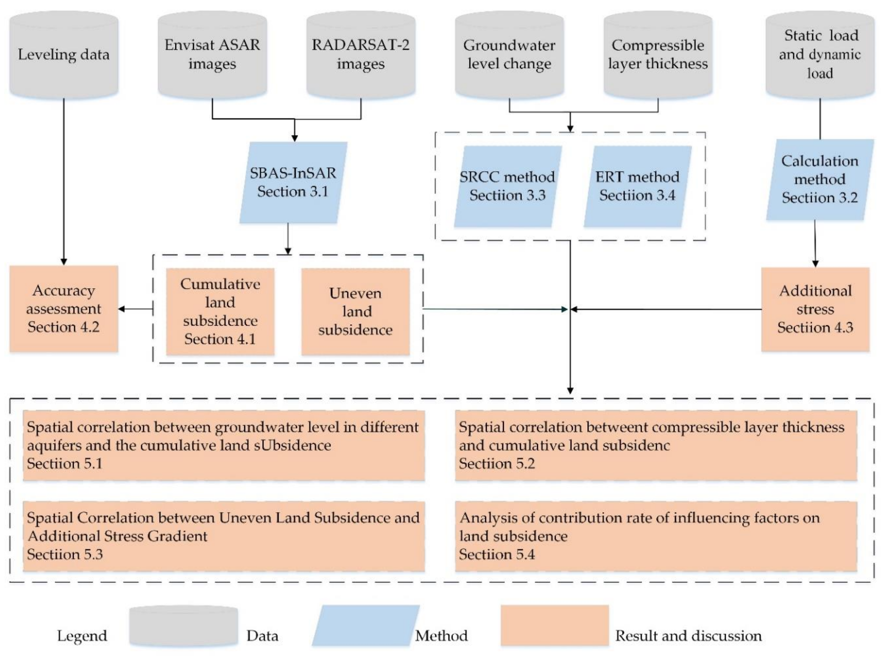
Figure 2 shows the flowchart of this research. First, we adopted the SBAS-InSAR method for the EA and R2 images to obtain land subsidence information and to validate the SBAS-InSAR results using the leveling benchmark monitoring results. Second, the additional stress engendered from the static and dynamic loads was calculated. Third, the contribution rate of the influencing factors to cumulative and uneven land subsidence was analyzed by Spearman’s rank correlation coefficient (SRCC) and extremely randomized trees (ERT) machine learning methods.

3.1. SBAS-InSAR Processing for the EA and R2 Datasests

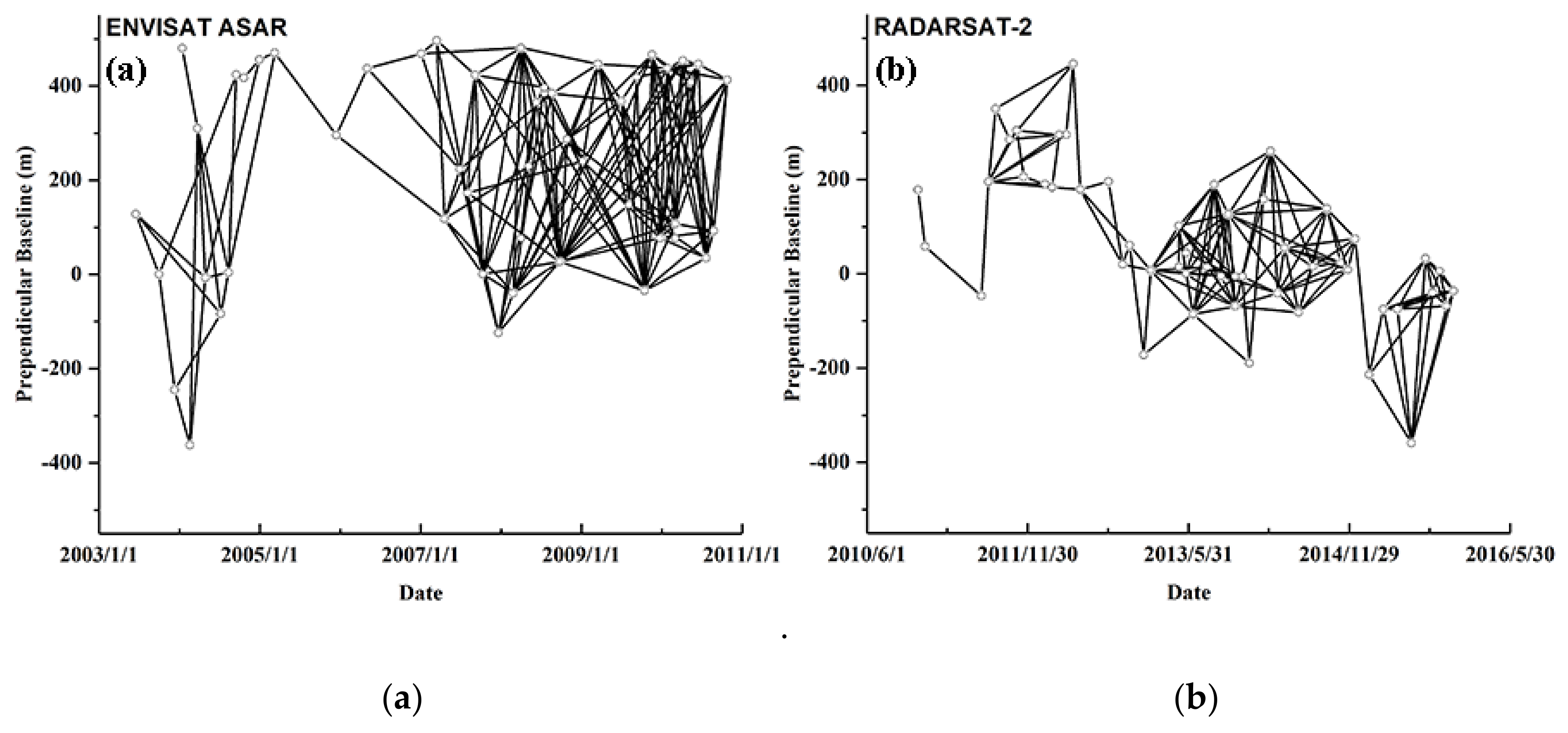
The SBAS-InSAR method has been widely used for deriving slow ground deformation [15,26]. To maximize the correlations between interferograms, the SBAS-InSAR method was used to obtain the minimum value of the separation in the Doppler frequency and in the time intervals of acquisition pairs. The SBAS-InSAR method was also used in the GAMMA software to obtain ground deformation. First, the SAR images were registered to the same master image within each stack. Then, 267 interferograms were generated for the EA data when the temporal and perpendicular baseline thresholds were set as 500 days and 500 m, respectively. For the R2 data, 163 interferograms were created when the temporal and perpendicular baseline thresholds were set as 500 days and 500 m, respectively. Figure 3 shows the network of the spatial and temporal baselines for the SBAS interferograms. The temporal coherence threshold was set as 0.7, which has been widely applied in InSAR applications. The least-squares method was used in the phase unwrapping, and the threshold was set as half of the satellite wavelength. The spatial filters were used to eliminate the phase noise. Finally, the ground deformation information along the line-of-sight (LOS) direction was obtained. Considering that the horizontal deformation in the BP can be neglected [21], the land deformation velocity was estimated by using Equation (1).
V = V l o s c o s φ
where V and V l o s represent the deformation rate in the vertical (i.e., land subsidence) and LOS directions, respectively, and φ is the incidence angle of the radar satellite sensor.

3.2. Additional Stress Engendered from Static and Dynamic Loads

Based on the building information provided by the BIGMAP software, we learned that on average, buildings in Beijing weigh 1300 kg/m2 and bear 200 kg/m2. Furthermore, the soil weighs 2000–2200 kg/m2 in the range of 0–100 m underground, and the depth of the foundations of buildings should not be less than 1/15 the building’s height when buildings are greater than seven stories. The weight of the building was calculated by multiplying the area of the building by 1500 kg and then subtracting the weight of the soil replaced by the foundation. To simplify the calculation process, the dynamic load of subways and expressways was considered as the equivalent static load. According to the data provided by the Beijing Mass Transit Railway Operation Corp (Table 1), the equivalent static load of each metro line crossing the study area was calculated using Equation (2) [27].
P E S = 0.26 P E ( 1 + 0.004 V E )
where P E and V E represent the load and operating speed of metro vehicles, respectively, and P E S is the equivalent static load of metro vehicles.
According to the information provided by the Beijing Traffic Management Bureau (Table 2), the equivalent static load of different cars, buses, and trucks was calculated using Equation (2). Based on the proportion, the average equivalent static load of expressways was calculated using Equation (3).
P V S = i = 1 n M i P i
where n is the number of types of vehicle, M i and P i represent the proportion and equivalent static load of cars, buses and trucks, respectively, and P V S is the average equivalent static load of expressways.
We generated a series of grid points with an interval of 10 m along the longitude, latitude, and vertical dimensions in World Geodetic System 1984 (WGS84). The additional stress of each point in the grid was calculated by summing the additional stress engendered from the static and dynamic loads by using Equation (4). Table 3 shows the meaning of each parameter in Equation (4). Additional stress and stress gradient maps can be obtained by using the IDW interpolation tool.
σ = P b + P t + P v P b = i = 1 n 3 P i 2 π ( Z Z i ) 3 ( X X i ) 2 + ( Y Y i ) 2 + ( Z Z i ) 2 5 / 2 P t = j = 1 m 3 P j 2 π ( Z Z j ) 3 ( X X j ) 2 + ( Y Y j ) 2 + ( Z Z j ) 2 5 / 2 P v = k = 1 e 3 P k 2 π ( Z Z k ) 3 ( X X k ) 2 + ( Y Y k ) 2 + ( Z Z k ) 2 5 / 2

3.3. Spearman’s Rank Correlation Coefficient

SRCC, proposed by Spearman and widely used in the field of statistics, is a statistical index that reflects the correlation between two groups of variables. The value of SRCC ranges from −1 to 1, and the larger the value, the stronger the correlation. Compared to Pearson’s product motion correlation coefficient (PMMCC), it overcomes the disadvantage of variables following normal distribution. In this study, we used SRCC to quantitatively measure the correlations among the ground water level, the thickness of compressible layer, the additional stress engendered from static and dynamic loads, and the land subsidence. SRCC can be calculated using Equation (5).
p = 1 6 i = 1 n d i 2 n ( n 2 1 )
where n represent the number of variables in the first group and d i is the difference of the rank of the corresponding variable in the second group.

3.4. Extremely Randomized Trees

As an extension of the random forest method, the extremely randomized trees (ERT) method is an efficient supervised machine learning algorithm that is widely used in regression and classification problems. The ERT method can obtain more reliable results than the random forest method by using all of the sample sets in the training process. Based on decision tree learning, ERT is a more advanced algorithm that contains many decision trees. As an ensemble machine learning method, the ERT method has the following advantages. (1) This method is unexcelled in accuracy among current algorithms, because its results are determined by voting of the results of the many decision trees included in ERT. (2) ERT can handle thousands of input variables with multi-dimensional characteristics without variable deletion. (3) ERT can evaluate the importance of variables in the process of algorithm implementation. (4) This method is very efficient, especially for large datasets.
In this paper, the ERT algorithm was implemented by using the sklearn.ensemble library in Python. We used the ExtraTreesRegressor regression model in the sklearn.ensemble library to quantitatively measure the contribution rate of changes in the level of groundwater in different aquifers, the thickness of compressible layers, and additional stress engendered from static and dynamic loads to cumulative and uneven land subsidence. The results of the ERT algorithm and the SRCC method were cross-validated.

4. Results

4.1. Surface Deformation Measured by SBAS-InSAR in Two Time Periods

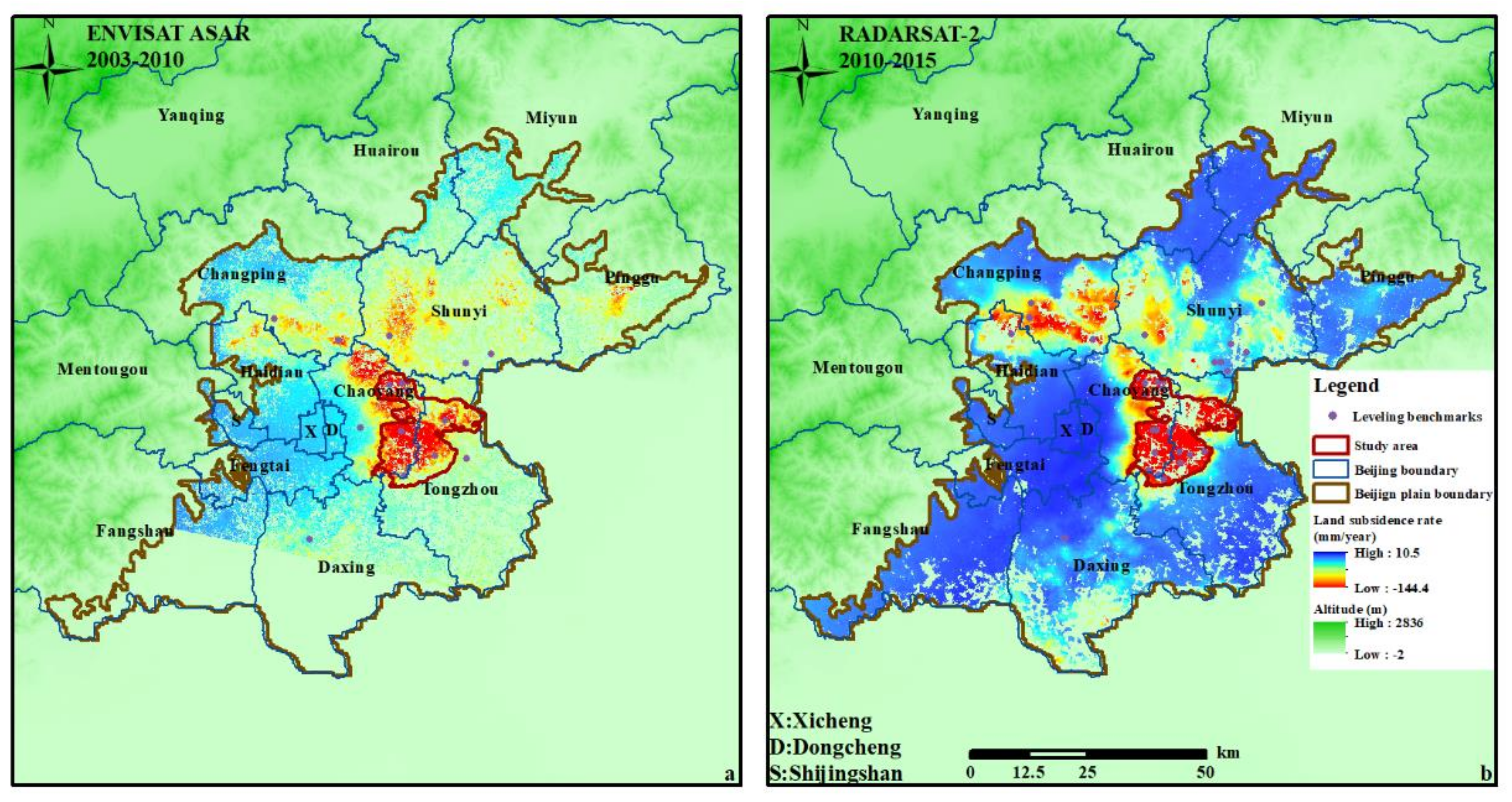
Based on the surface displacement information measured by SBAS-InSAR, a land subsidence rate distribution map during the observation period was obtained for the BP. Figure 4 shows that land subsidence is widely distributed in the BP, and the spatial discrepancy is huge. The areas with serious land subsidence are mainly distributed in the middle and east of the Chaoyang District, the northwest of the Tongzhou District, the middle and south of the Changping District, the west of the Shunyi District, and the south of the Daxing District. From June 2003 to August 2010, 19,090 pixels were detected in the study area based on the EA data, with a density of 181 pixel/km2, and the average land subsidence rate varied from −110.7 to +8.3 mm/year. For the R2 data, we detected 17,605 pixels in the study area from November 2010 to November 2015, with a density of 167 pixel/km2, and the average land subsidence rate varied from −144.4 to +10.5 mm/year.
Figure 5 shows that the discrepancy of the land subsidence is obvious from 2003 to 2015 in the LDD land subsidence funnel. To further study the temporal and spatial evolution patterns of the land subsidence, we obtained the maximum land subsidence rate and area with a land subsidence rate greater than 100 mm/year. Figure 6 shows that land subsidence experienced a rapid expansion period from 2004 to 2007. The maximum land subsidence rate and area with a land subsidence rate greater than 100 mm/year increased from 111.8 to 143.5 mm/year and from 0.1 to 24.9 km2, respectively. From 2007 to 2008, land subsidence showed a decreasing trend, in which the maximum land subsidence rate and area with a land subsidence rate greater than 100 mm/year decreased from 143.5 to 126.4 mm/year and from 24.9 to 8.2 km2, respectively. Land subsidence developed rapidly from 2008 to 2010, with the maximum land subsidence rate and area with a land subsidence rate greater than 100 mm/year increasing to 157.6 mm/year and 68.9 km2, respectively. From 2010 to 2011, the land subsidence showed a decreasing trend, in which the maximum land subsidence rate and area with a land subsidence rate greater than 100 mm/year decreased to 134.7 mm/year and 63.1 km2, respectively. Land subsidence remained in a relatively stable state from 2011 to 2015, during which time the maximum land subsidence rate and area with a land subsidence rate greater than 100 mm/year rarely changed.

4.2. Accuracy Assessment of the SBAS-InSAR Results

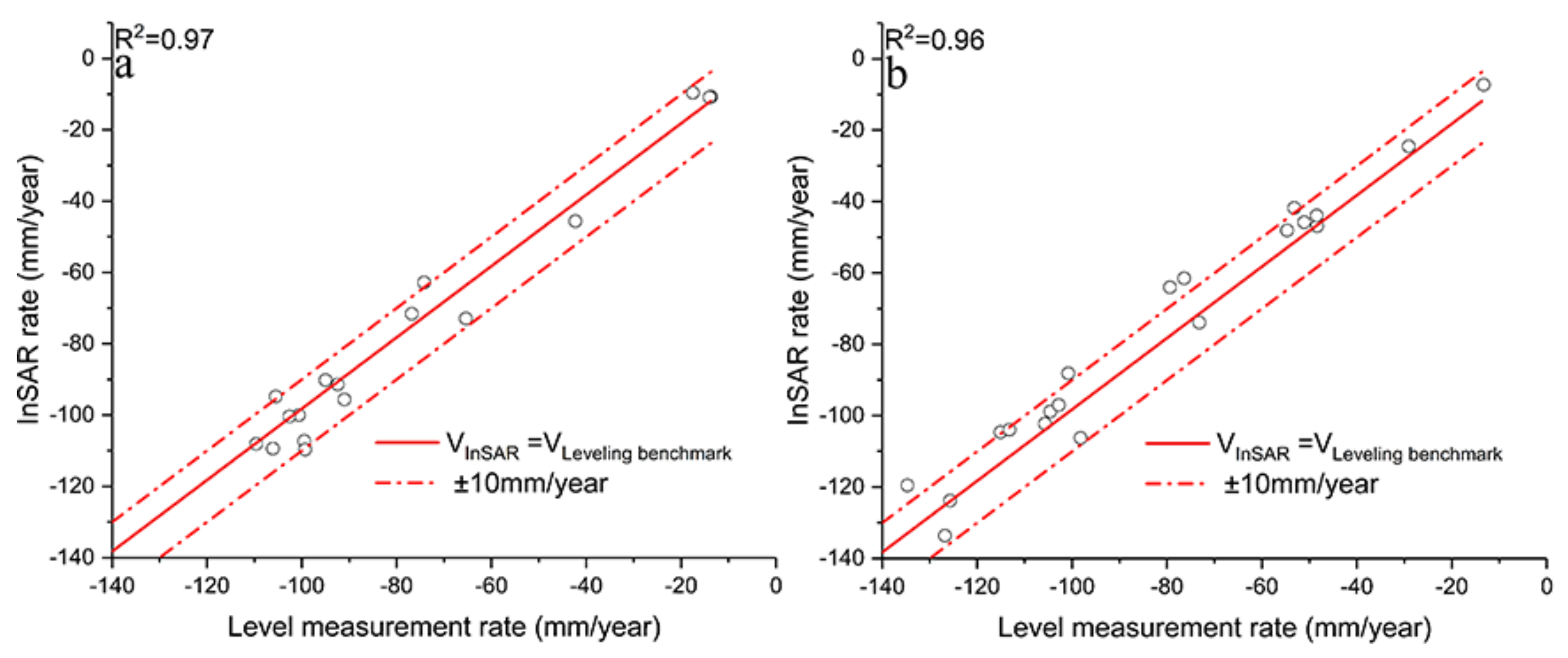
As shown in Figure 4, 37 leveling benchmarks evenly distributed in the BP were selected for accuracy assessment of the SBAS-InSAR results—that is, 17 and 20 leveling benchmarks measuring precise ground deformation data during 2003–2010 and 2013–2015 periods, respectively. The leveling benchmarks were set as datum points, and the monitoring points within 200 m of the leveling benchmarks were extracted. The average deformation rate of each leveling benchmark was compared to the average land subsidence rate of the extracted points around said leveling benchmark from 2003 to 2010 and 2013 to 2015. Figure 7a,b show that the correlation coefficients between the leveling benchmark monitoring results and the SBAS-InSAR results during the 2003–2010 and 2013–2015 periods were 0.97 and 0.96, respectively.

4.3. Acquisition of Additional Stress Engendered from Static and Dynamic Loads

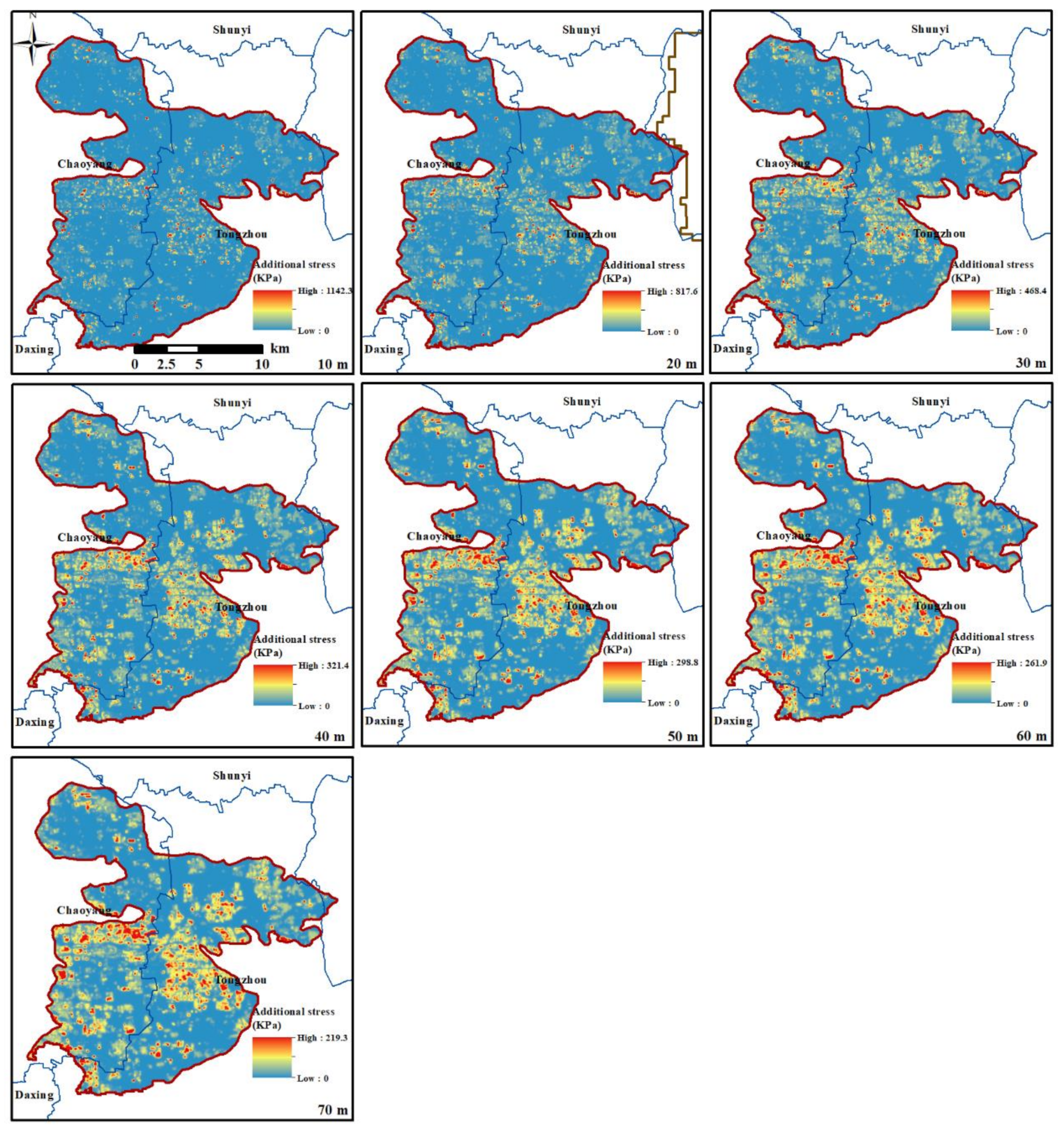
The additional stress information engendered from static and dynamic loads in the LDD land subsidence funnel was obtained by using the method outlined in Section 3.2. This additional stress will not cause significant land subsidence in this stratum when the additional stress is less than 20% of the stress engendered from the gravity of the soil above the depth [28]. Table 4 shows the detailed parameters of the soil in the LDD land subsidence funnel, while Figure 8 shows that the maximum value of the additional stress engendered from the static and dynamic loads is less than 20% of the stress engendered from the gravity of the soil when the depth is greater than 65.1 m by assuming that the density of the soil above this depth is 1930 kg/m3. This result reveals that the influence of the depth of additional stress engendered from the static and dynamic loads was 65.1 m in the LDD land subsidence funnel.
As shown in Figure 9, the superposition of additional stress engendered from the static and dynamic loads in the LDD land subsidence funnel obviously enhanced as the depth increased. Figure 8 and Figure 9 show that the additional stress decreased sharply as the depth increased between 10 and 70 m. These results indicate that the influence of additional stress engendered from static and dynamic loads on land subsidence may decrease as the depth increase, especially for uneven land subsidence.

5. Discussion

5.1. Evaluating the Spatial Correlation between Groundwater Level in Different Aquifers and the Cumulative Land Subsidence

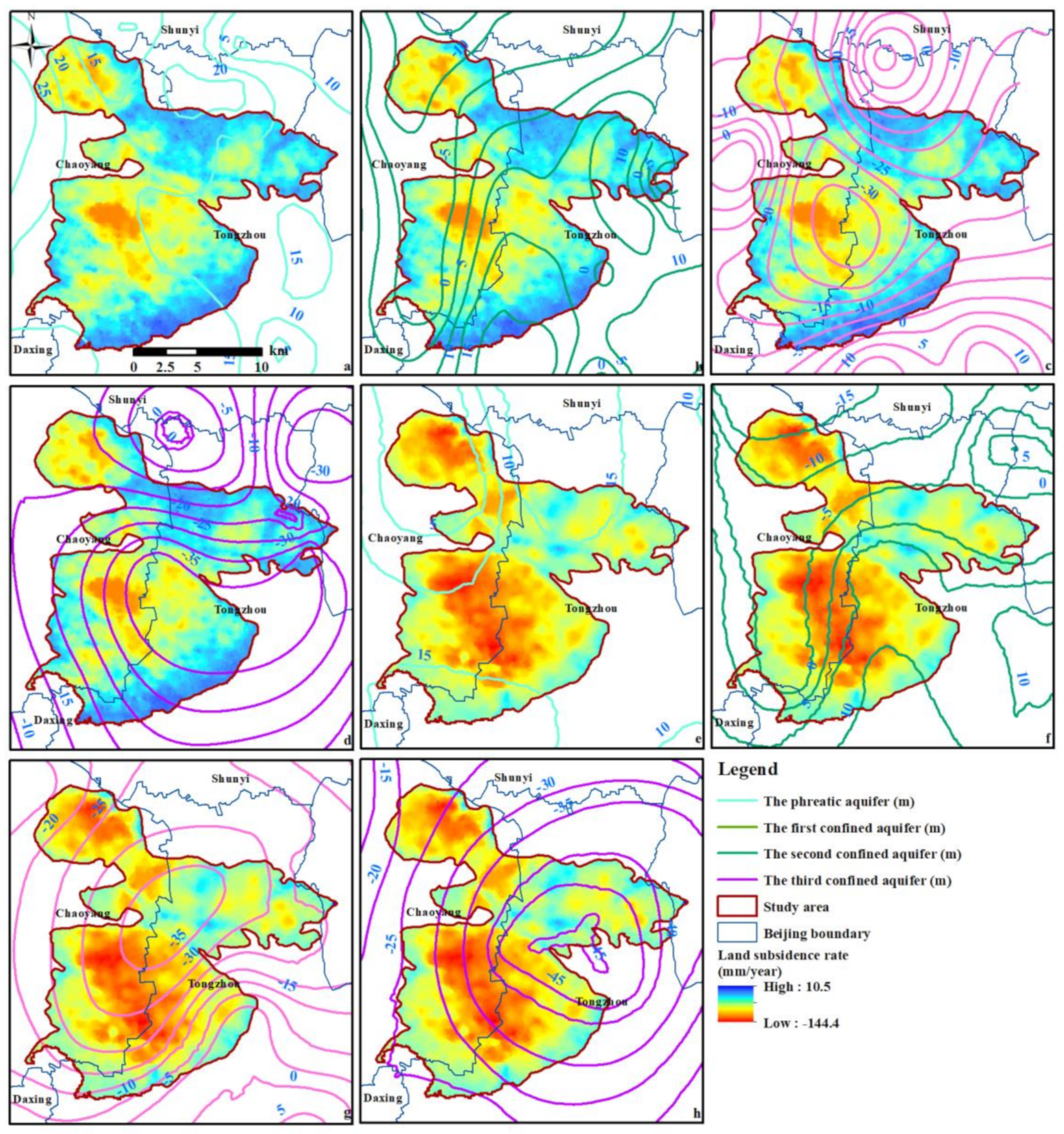
Previous studies have shown that land subsidence in the LDD land subsidence funnel is mainly caused by overexploitation of groundwater [6,24]. Analysis of the spatial correlation between the groundwater level in different aquifers and cumulative land subsidence was implemented in two different time periods.
We used the IDW interpolation method for the surface deformation information measured by SBAS-InSAR technique to obtain land subsidence rate maps during the 2003–2010 and 2010–2015 periods. Overlay analysis was applied to explore the spatial correlation between the groundwater level in different aquifers and the land subsidence rate. The spatial distribution of the second confined aquifer was more consistent with cumulative land subsidence than that of the phreatic aquifer, the first confined aquifer, and the third confined aquifer from 2003 to 2010 (Figure 10). From 2003 to 2010, a large amount of the groundwater from the second confined aquifer was extracted for agricultural irrigation. From 2010 to 2015, groundwater exploitation from the phreatic aquifer increased, while the exploitation of the second confined aquifer decreased; thus, the groundwater level of the phreatic aquifer decreased significantly during this period. This result reveals that the contribution of the phreatic aquifer to cumulative land subsidence may have increased.
In order to further study the spatial correlation between the groundwater level in different aquifers and cumulative land subsidence, the SRCC between the land subsidence rate and the groundwater level in different aquifers was calculated in two different time periods. Table 5 shows that the SRCC between the groundwater level in the second aquifers and the land subsidence rate was 0.67, which was significantly larger than that of the other aquifers from 2003 to 2010. This result indicates that the second confined aquifer was the main layer contributing to cumulative land subsidence from 2003 to 2010. The SRCC between the groundwater level in the phreatic aquifers and the land subsidence rate was 0.5 from 2010 to 2015, which indicates that the phreatic aquifer was the main layer that contributed to cumulative land subsidence during this period.

5.2. Evaluation of the Spatial Correlation betweent Compressible Layers of Different Thicknesses and Cumulative Land Subsidence

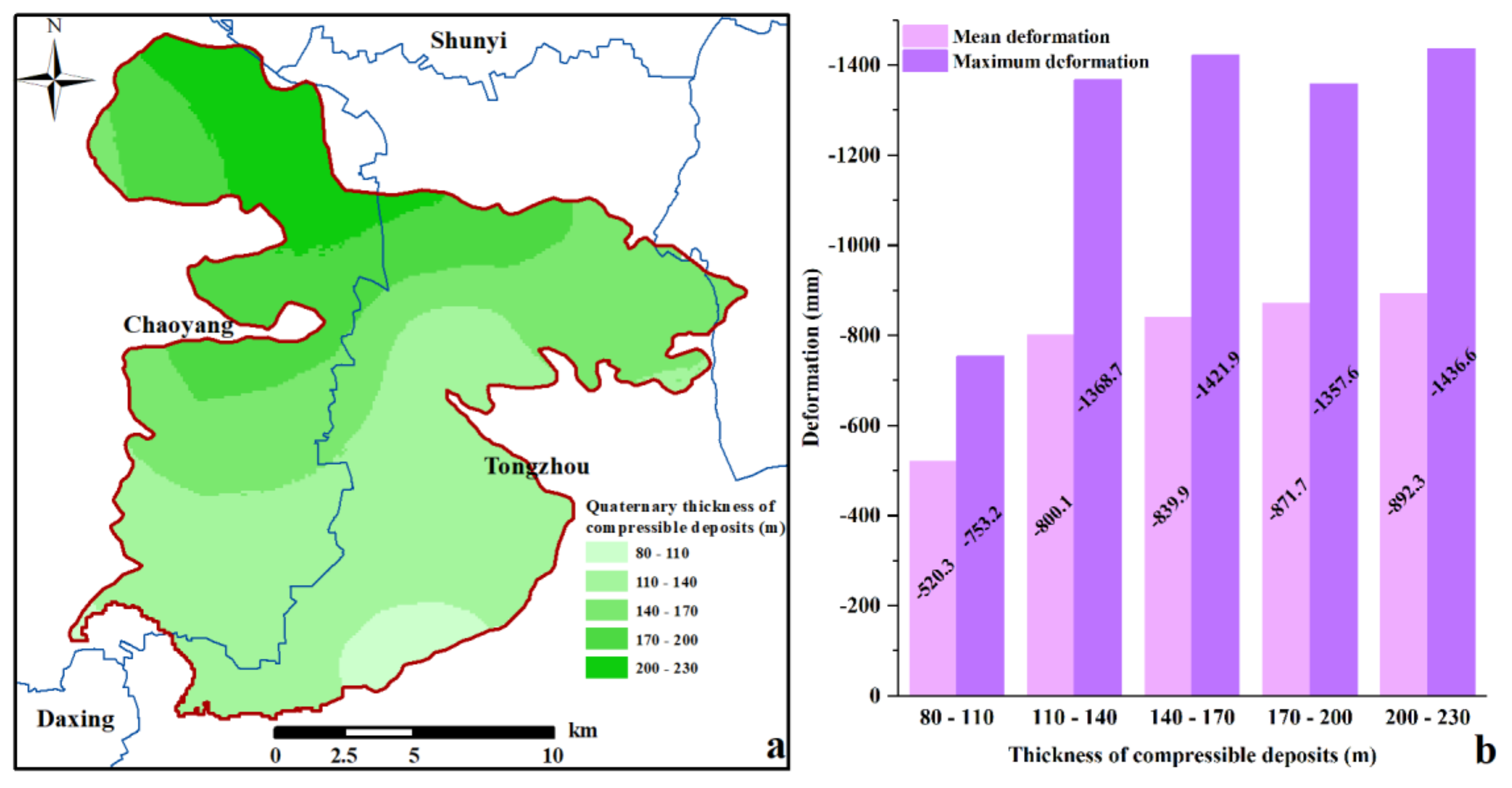
The existence of compressible layers provides basic geological conditions for the occurrence of land subsidence. Figure 11a shows the distribution of compressible layers of different thicknesses. We divided the compressible layers into five categories and obtained the maximum and mean cumulative deformation from 2003 to 2015 in each compressible layer of a different thickness. The results show that the maximum and the mean cumulative deformation increased with the increase in the thickness of the compressible layers, except for the maximum cumulative deformation at 140–170 m, which was greater than the maximum cumulative deformation at 170–200 m.
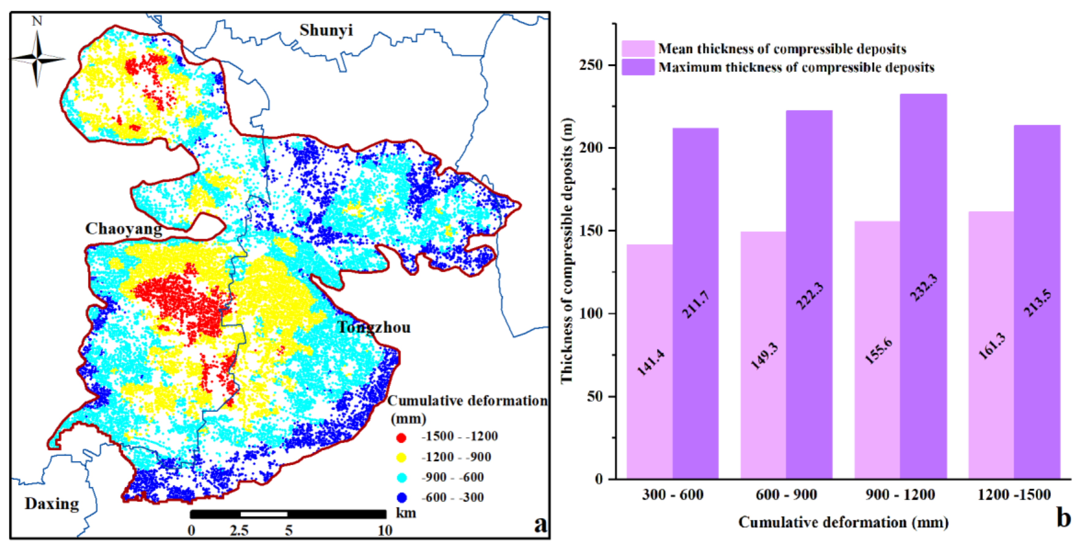
To further study the spatial correlation between compressible layers of different thicknesses and cumulative land subsidence, the cumulative deformation from 2003 to 2015 was divided into four categories, and the maximum and mean thicknesses of the compressible layers in each cumulative deformation were calculated. Figure 12b shows that the maximum and mean thicknesses of the compressible layers increased as the cumulative deformation increased, except for the maximum thickness at 900–1200 mm, which was greater than the maximum thickness at 1200–1500 mm.

5.3. Evaluation of the Spatial Correlation between Uneven Land Subsidence and Additional Stress Gradients

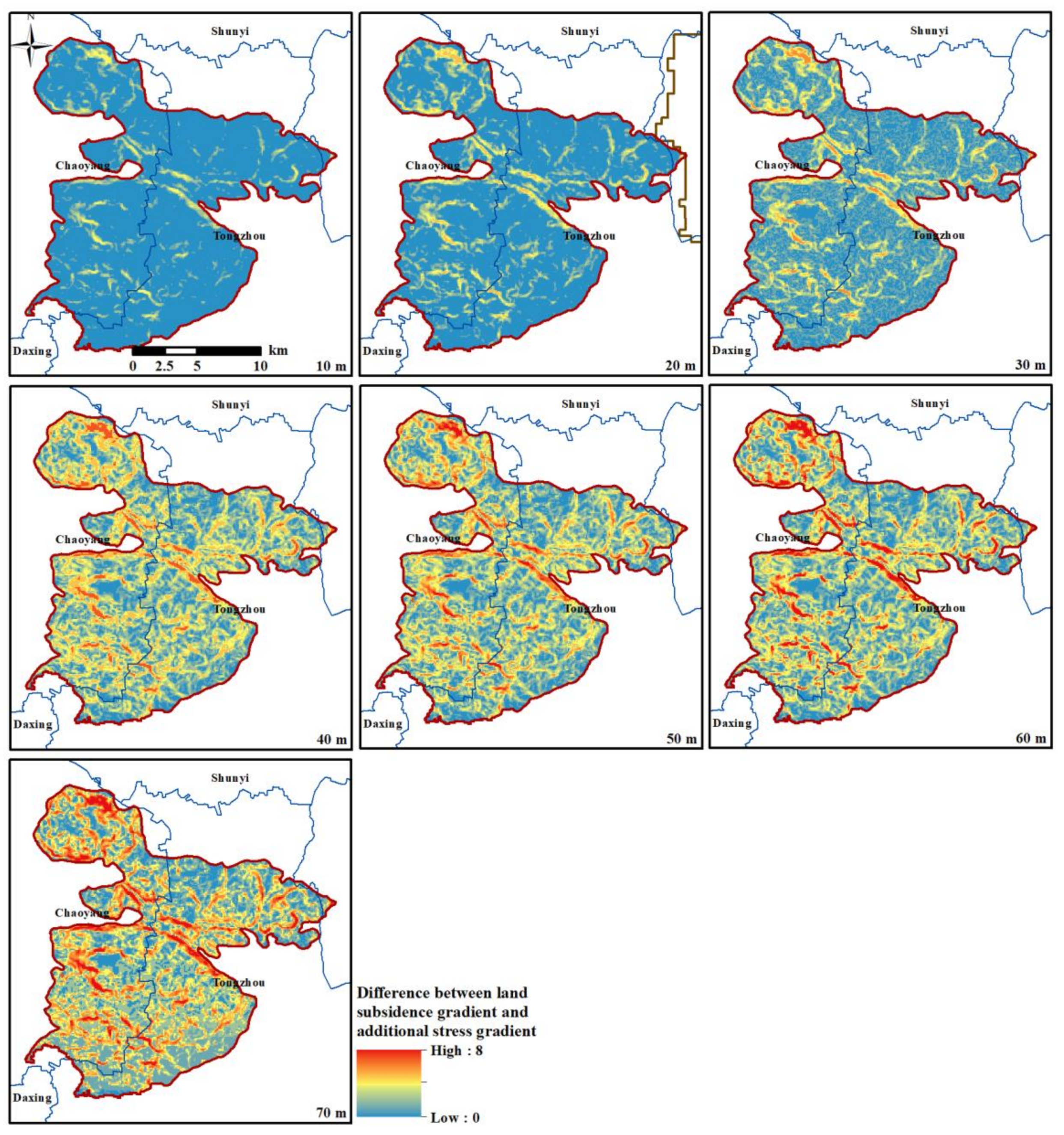
The additional stress gradient at different depths and the land subsidence rate gradient were calculated and both were divided into nine categories. Figure 13 shows the distribution of the differences between the land subsidence rate gradient and the additional stress gradient with depths less than 65.1 m. The results show that the differences increased rapidly as the depth increased, which indicates that the influence of additional stress engendered from static and dynamic loads on uneven land subsidence decreased rapidly as the depth increased. This can be explained by the fact that the superposition of the additional stress enhanced as the depth increased, while the differences between the additional stresses decreased as the depth increased.
We calculated the SRCC between the land subsidence rate gradient and the additional stress gradient, the gradient of compressible layers of different thickness, and the groundwater level gradient in different aquifers from 2003 to 2010 and 2010 to 2015. Table 6 shows that the SRCC between the land subsidence rate gradient and the additional stress gradient was significantly larger than that of the other factors from 2003 to 2010 and 2010 to 2015. This result indicates that additional stress plays an important role in controlling uneven land subsidence. The SRCC between the groundwater level gradient in the phreatic aquifer and the land subsidence rate gradient increased from 2003 and 2015, which indicates that the contribution of the phreatic aquifer to uneven subsidence increased.

5.4. Quantitative Analysis of the Contribution Rate of the Influencing Factors on Land Subsidence Using the ERT Method

In this study, we selected 36,695 pixels detected by the SBAS-InSAR technique as research data to quantify the contribution rate of the influencing factors to land subsidence using the ERT method. To automatically optimize the ERT model parameters, the coordinate descent method was used in this study. Of the research data, 70% were selected as the training data, and the rest were selected as the verification data.

5.4.1. Contribution Rate of the Influencing Factors to Cumulative Land Subsidence

We selected the cumulative deformation from 2003 to 2010 and 2010 to 2015 as the dependent variable, while the groundwater level in the different aquifers, the thickness of compressible layers, and additional stress engendered from static and dynamic loads in same time period were the explanatory variables. Figure 14 shows that the contribution rate of the second confined aquifer was 49.3% from 2003 to 2010, which indicates that the second confined aquifer was the main contribution layer during this period. We found that the influence of the second confined aquifer on cumulative land subsidence dramatically decreased from 2010 to 2015, with a contribution rate of 23.4%. The contribution rate of the phreatic aquifer increased sharply from 2.7% between 2003 and 2010 to 33.9% between 2010 and 2015, indicating that the phreatic aquifer played an important role in the evolution of land subsidence from 2010 to 2015. These results are consistent with those of the SRCC method. The contribution rate of the static and dynamic loads was 2.5% between 2003 and 2010 and 2.6% between 2010 and 2015. These results indicate that the influence of the static and dynamic loads on cumulative land subsidence was slight. We found that the contribution rate of compressible layers of different thicknesses was 12.4% between 2003 and 2010 and 13.6% between 2010 and 2015, and that the contribution rate of the first confined aquifer obviously decreased from 24.5% between 2003 and 2010 to 14.2% between 2010 and 2015; Meanwhile, the contribution rate of the third confined aquifer increased from 8.6% between 2003 and 2010 to 12.3% between 2010 and 2015, which can be explained by the fact that the upper part of the third confined aquifer gradually became the main mining layer. The contribution rate of the third confined aquifer is expected to increase in the future. The verification results revealed that the accuracy of the ERT model reached 97.7% between 2003 and 2010 and 98.8% between 2010 and 2015.

5.4.2. Contribution Rate of the Influencing Factors to Uneven Land Subsidence

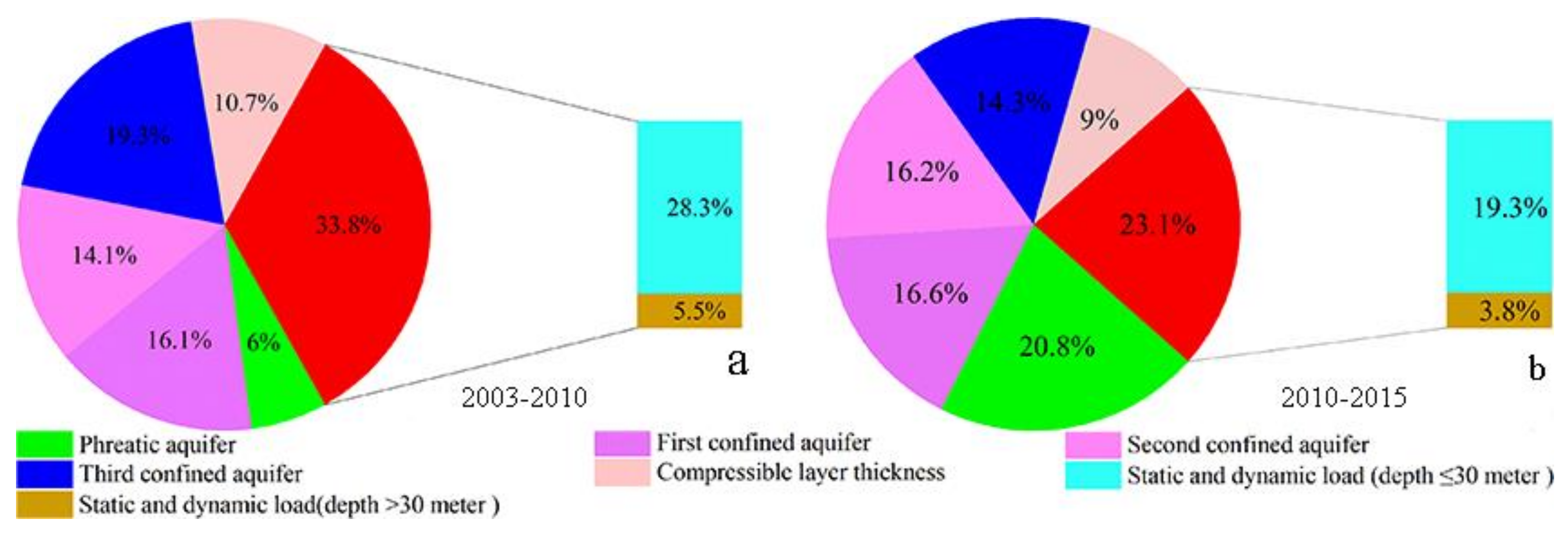
We calculated the gradient of cumulative deformation to represent uneven deformation and explored the relationship between uneven deformation and its influencing factors. The gradient of cumulative deformation from 2003 to 2010 and 2010 to 2015 was selected as the dependent variable and groundwater level gradient in the different aquifers, the gradient of compressible layers of different thicknesses, and the gradient of additional stress engendered from static and dynamic loads were selected as the explanatory variables. Figure 15a shows that the contribution rate of the static and dynamic loads accounted for 33.8% from 2003 to 2010, including 28.3% with a depth of less than 30 m and 5.5% with a depth greater than 30 m. This result indicates that the additional stress engendered from static and dynamic loads plays an important role in controlling uneven land subsidence, especially in the stratum with a depth of less than 30 m. We found that the contribution rates of the phreatic aquifer, the first confined aquifer, the second confined aquifer, the third confined aquifer, and the compressible layers of different thicknesses were 6%, 16.1%, 14.1%, 19.3%, and 10.7%, respectively from 2003 to 2010. The contribution rate of the phreatic aquifer increased sharply from 6% between 2003 and 2010 to 20.8% between 2010 and 2015. This result is consistent with that of SRCC to some extent. We found that the contribution rate of the static and dynamic loads decreased from 33.8% between 2003 and 2010 to 23.1% between 2010 and 2015, but it still accounted for the largest proportion. The accuracy of the ERT model was 82.3% from 2003 to 2010 and 85.4% from 2010 to 2015.

6. Conclusions

In this study, we obtained surface deformation information from June 2003 to November 2015 in the BP by applying the SBAS-InSAR technique to 47 EA images and 48 R2 images, and then we verified the accuracy of the SBAS-InSAR results. Based on the ground deformation monitoring results, we analyzed the evolution pattern of land subsidence in the LDD land subsidence funnel. The spatial correlation between land subsidence and its influencing factors (i.e., the groundwater level in the phreatic aquifer, the first confined aquifer, the second confined aquifer, and the third confined aquifer, the compressible layers of different thicknesses, and the additional stress engendered from static and dynamic loads) were explored using the overlay analysis method, the spatial statistics method, the SRCC method, and the ERT method in machine learning. The following conclusions can be drawn.
(1)
The maximum land subsidence rate reached 110.7 mm/year and 144.4 mm/year during the 2003–2010 and 2010–2015 periods, respectively. Land subsidence experienced rapid expansion from 2003 to 2010. The maximum land subsidence rate and area with a land subsidence rate greater than 100 mm/year increased from 111.8 to 157.6 mm/year and from 0.1 to 68.9 km2, respectively. Land subsidence showed a decreasing trend from 2010 to 2011 and then remained in a relatively stable stage from 2011 to 2015. The SBAS-InSAR results agree well with the leveling benchmark monitoring results, and the correlation coefficient was 0.97 from 2003 to 2010 and 0.96 from 2013 to 2015.
(2)
We found that the greatest contribution to cumulative land subsidence was the second confined aquifer from 2003 to 2010, with a contribution rate of 49.3%. However, its contribution rate decreased to 23.4% from 2010 to 2015. The phreatic aquifer was the main contribution layer from 2010 to 2015, with a contribution rate of 33.9%. The contribution rate of the third confined aquifer increased from 2003 to 2015 due to the upper part of third confined aquifer gradually becoming the main mining layer. We innovatively calculated additional stress to represent static and dynamic load information to show the superposition of additional stress; however, the influence of additional stress engendered from the static and dynamic loads on cumulative land subsidence was slight.
(3)
The contribution rate of the static and dynamic loads to uneven land subsidence was 33.8% from 2003 to 2010 and 23.1% from 2010 to 2015, accounting for the largest proportion. The contribution rate of static and dynamic loads with depths of less than 30 m accounted for more than 80% of the total contribution rate of said static and dynamic loads. This result shows that said additional stress has a significant effect on the distribution of uneven settlement, especially in the stratum with a depth of less than 30 m.
In summary, the spatial distribution of cumulative land subsidence is mainly affected by geological conditions, and the additional stress engendered from static and dynamic loads has a significant impact on the distribution of uneven land subsidence. This research has improved our understanding of the relationship between land subsidence and its influencing factors.

Supplementary Materials

The following are available online at https://www.mdpi.com/2072-4292/12/18/2963/s1.

Author Contributions

F.L. completed the experiments, performed the algorithm, and wrote the original paper. H.G. provided vital guidance and support. B.C. provided data and crucial support. C.Z. and L.G. made critical suggestions on writing this paper. All authors have read and agreed to the published version of the manuscript.

Funding

This research was funded by The National Natural Science Foundation of China (No. 41930109/ D010702, 41771455/ D010702), Beijing Outstanding Young Scientist Program (No. BJJWZYJH01201910028032), Natural Science Foundation of Beijing Municipality (No.8182013), and Beijing Youth Top Talent Project, a program of Beijing Scholars and National “Double-Class” Construction of University Projects.

Acknowledgments

We thank the European Space Agency for providing EA data and the Canadian Space Agency for providing R2 data. We thank the National Aeronautics and Space Administration for proving the SRTM DEM data. We also thank BIGMAP for providing building information.

Conflicts of Interest

The authors declare no conflict of interest.

References

  1. Hu, R.L.; Yue, Z.Q.; Wang, L.U.; Wang, S.J. Review on current status and challenging issues of land subsidence in China. Eng. Geol. 2004, 76, 65–77. [Google Scholar] [CrossRef]
  2. Castellazzi, P.; Garfias, J.; Martel, R.; Brouard, C.; Rivera, A. InSAR to support sustainable urbanization over compacting aquifers: The case of Toluca Valley, Mexico. Int. J. Appl. Earth Obs. Geoinf. 2017, 63, 33–44. [Google Scholar] [CrossRef]
  3. Galloway, D.; Hudnut, K.; Ingebritsen, S.; Ingebritsen, S.; Phillips, S.; Peltzer, S.; Rogez, F.; Rosen, P. Detection of aquifer system compaction and land subsidence using interferometric synthetic aperture radar, Antelope Valley, Mojave Desert, California. Water Resour. Res. 1998, 34, 2573–2585. [Google Scholar] [CrossRef]
  4. Strozzi, T.; Caduff, R.; Wegmüller, U.; Raetzo, H.; Hauser, M. Widespread surface subsidence measured with satellite SAR interferometry in the Swiss alpine range associated with the construction of the Gotthard BaseTunnel. Remote Sens. Environ. 2017, 190, 1–12. [Google Scholar] [CrossRef]
  5. Ng, A.H.M.; Ge, L.; Li, X.; Abidin, H.Z.; Andreas, H.; Zhang, K. Mapping land subsidence in Jakarta, Indonesia using persistent scatterer interferometry (PSI) technique with ALOS PALSAR. Int. J. Appl. Earth Obs. Geoinf. 2012, 18, 232–242. [Google Scholar] [CrossRef]
  6. Gao, M.; Gong, H.; Chen, B.; Li, X.; Zhou, C.; Min, S.; Yuan, S.; Zheng, C.; Duan, G. Regional Land Subsidence Analysis in Eastern Beijing Plain by InSAR Time Series and Wavelet Transforms. Remote Sens. 2018, 10, 365. [Google Scholar] [CrossRef] [Green Version]
  7. Samsonov, S.V.; Oreye, N.; Gonzalez, P.J.; Tiampo, K.F.; Ertolahti, L.; Clague, J.J. Rapidly accelerating subsidence in the Greater Vancouver region from two decades of ERS-ENVISAT-RADARSAT-2 DInSAR measurements. Remote Sens. Environ. 2014, 143, 180–191. [Google Scholar] [CrossRef] [Green Version]
  8. Du, Z.; Ge, L.; Ng, A.; Yang, X.; Liyuan, L. Correlating the subsidence pattern and land use in Bandung, Indonesia with both Sentinel-1/2 and ALOS-2 satellite images. Int. J. Appl. Earth Obs. Geoinf. 2018, 7, 54–68. [Google Scholar] [CrossRef]
  9. Zhou, C.; Gong, H.; Chen, B.; Gao, M.; Cao, Q.; Cao, J.; Duan, L.; Zuo, J.; Shi, M. Land Subsidence Response to Different Land Use Types and Water Resource Utilization in Beijing-Tianjin-Hebei, China. Remote Sens. 2020, 12, 457. [Google Scholar] [CrossRef] [Green Version]
  10. Yu, H.; Gong, H.; Chen, B.; Liu, K.; Gao, M. Analysis of the influence of groundwater on land subsidence in Beijing based on the geographical weighted regression (GWR) model. Sci. Total Environ. 2020, 738, 139405. [Google Scholar] [CrossRef]
  11. Chen, B.; Gong, H.; Chen, Y.; Li, X.; Zhou, C.; Lei, K.; Zhu, L.; Duan, L.; Zhao, X. Land subsidence and its relation with groundwater aquifers in Beijing Plain of China. Sci. Total Environ. 2020, 735, 139111. [Google Scholar] [CrossRef]
  12. Zuo, J.; Gong, H.; Chen, B.; Liu, K.; Zhou, C.; Ke, Y. Time-series evolution patterns of land subsidence in the eastern Beijing Plain, China. Remote Sens. 2019, 11, 539. [Google Scholar] [CrossRef] [Green Version]
  13. Yang, Q.; Ke, Y.; Zhang, D.; Chen, B.; Gong, H.; Lv, M.; Zhu, L.; Li, X. Multi-Scale Analysis of the Relationship between Land Subsidence and Buildings: A Case Study in an Eastern Beijing Urban Area Using the PS-InSAR Technique. Remote Sens. 2018, 10, 1006. [Google Scholar] [CrossRef] [Green Version]
  14. Yan, X.; Gong, S.; Zeng, Z. Relationship between building density and land subsidence in Shanghai urban zone. Hydrogeol. Eng. Geol. 2002, 29, 21–25. [Google Scholar]
  15. Berardino, P.; Fornaro, G.; Lanari, R.; Sansosti, E. A new algorithm for surface deformation monitoring based on small baseline differential SAR interferograms. IEEE Trans. Geosci. Remote Sens. 2002, 40, 2375–2383. [Google Scholar] [CrossRef] [Green Version]
  16. Chaussard, E.; Wdowinski, S.; Cabral-Cano, E.; Amelung, F. Land subsidence in central Mexico detected by ALOS InSAR time-series. Remote Sens. Environ. 2014, 140, 94–106. [Google Scholar] [CrossRef]
  17. Chen, B.; Gong, H.; Lei, K.; Li, J.; Zhou, C.; Gao, M.; Guan, H.; Lv, W. Land subsidence lagging quantification in the main exploration aquifer layers in Beijing plain, China. Int. J. Appl. Earth Obs. Geoinf. 2019, 75, 54–67. [Google Scholar] [CrossRef]
  18. Abdollahi, S.; Pourghasemi, H.; Ghanbarian, G.; Safaeian, R. Prioritization of effective factors in the occurrence of land subsidence and its susceptibility mapping using an SVM model and their different kernel functions. Bull. Eng. Geol. Environ. 2019, 78, 4017–4034. [Google Scholar] [CrossRef]
  19. Rahmati, O.; Falah, F.; Naghibi, S.; Biggs, T.; Soltani, M.; Cerda, A.; Mohammadi, F.; Bui, T. Land subsidence modelling using tree-based machine learning algorithms. Sci. Total Environ. 2019, 672, 239–252. [Google Scholar] [CrossRef]
  20. Zamanirad, M.; Sarraf, A.; Sedghi, H.; Saremi, A.; Rezaee, P. Modeling the Influence of Groundwater Exploitation on Land Subsidence Susceptibility Using Machine Learning Algorithms. Nat. Resour. Res. 2020, 29, 1127–1141. [Google Scholar] [CrossRef]
  21. Zhou, C.; Gong, H.; Chen, B.; Li, X.; Li, J.; Wang, X.; Gao, M.; Si, Y.; Guo, L.; Shi, M.; et al. Quantifying the contribution of multiple factors to land subsidence in the Beijing Plain, China with machine learning technology. Geomorphology 2019, 335, 48–61. [Google Scholar] [CrossRef]
  22. Guo, L.; Gong, H.; Zhu, F.; Zhu, L.; Zhang, Z.; Zhou, C.; Gao, M.; Sun, Y. Analysis of the Spatiotemporal Variation in Land Subsidence on the Beijing Plain, China. Remote Sens. 2019, 11, 1170. [Google Scholar] [CrossRef] [Green Version]
  23. Chen, B.; Gong, H.; Li, X.; Lei, K.; Zhu, L.; Gao, M.; Zhou, C. Characterization and causes of land subsidence in Beijing, China. Int. J. Remote Sens. 2017, 38, 808–826. [Google Scholar] [CrossRef]
  24. Zhou, C.; Gong, H.; Chen, B.; Zhu, F.; Duan, G.; Gao, M.; Lu, W. Land subsidence under different land use in the eastern Beijing plain, China 2005-2013 revealed by InSAR timeseries analysis. GISci. Remote Sens. 2016, 53, 671–688. [Google Scholar] [CrossRef]
  25. Xue, X.; Wei, Y. Boussinesq-Mindlin united solution for pile-net compound foundation additional stress. High. Speed Railw. Technol. 2010, 1, 1–4. [Google Scholar]
  26. Ferretti, A.; Prati, C.; Rocca, F. Nonlinear subsidence rate estimation using permanent scatterers in differential SAR interferometry. IEEE Trans. Geosci. Remote Sens. 2000, 38, 2202–2212. [Google Scholar] [CrossRef] [Green Version]
  27. Liu, M.; Song, H.; Li, J. Long-term Settlement of Saturated Soft Clay under Subway Loading. Chin. J. Under Ground Space Eng. 2006, 2, 813–817. [Google Scholar]
  28. Li, F.; Gong, H.; Chen, B.; Gao, M.; Zhou, C. Subsidence monitoring with TerraSAR-X data in Beijing Central Business District and subway tunnelings, China. IAHS 2020, 382, 125–130. [Google Scholar] [CrossRef] [Green Version]
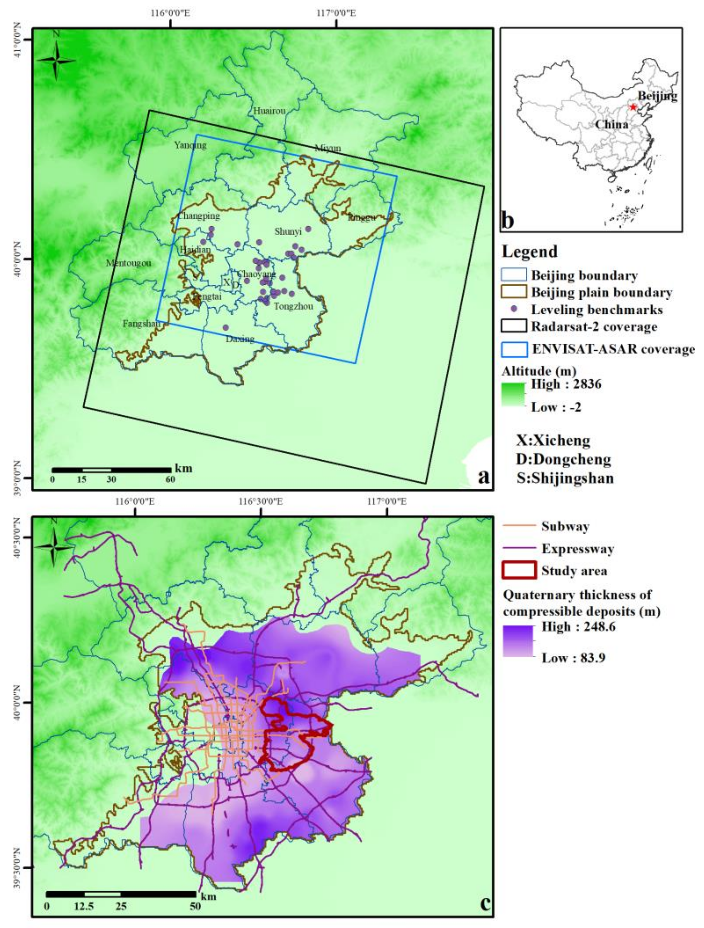
Figure 1. The geographical information of the study area. (a): The black and blue borders show the spatial coverage of RADARSAT-2 and ENVISAT ASAR, respectively. The violet dots represent the leveling benchmarks used to compare the deformation results derived by small baseline subset Interferometric Synthetic Aperture Radar (SBAS-InSAR) technique; (b): Location of Beijing; (c): Location of the study area (i.e., the Laiguangying–Dongbalizhuang–Dajiaoting (LDD) land subsidence funnel), the distribution of the traffic network, and the distribution of the thickness of Quaternary sediments in the Beijing Plain (BP).
Remotesensing 12 02963 g001
Figure 2. The flowchart of method of this research.
Remotesensing 12 02963 g002
Figure 3. The network of spatial and temporal baselines for SBAS interferograms (a): Based on ENVISAT ASAR data; (b): based on RADARSAT-2 data.
Remotesensing 12 02963 g003
Figure 4. Land subsidence rate maps in two time periods. (a): June 2003 to August 2010 based on ENVISAT ASAR (EA) data. (b): November 2010 to November 2015 based on RADARSAT-2 (R2) data.
Remotesensing 12 02963 g004
Figure 5. Annual deformation from June 2003 to November 2015. The black lines represent areas with a deformation rate >100 mm/year.
Remotesensing 12 02963 g005
Figure 6. Changes in the maximum land subsidence rate and areas with a land subsidence rate >100 mm/year from 2003 to 2015 in the LDD land subsidence funnel.
Remotesensing 12 02963 g006
Figure 7. Comparison of the SBAS-InSAR results, projected in the vertical direction, and the leveling measurement rates. (a): The accuracy assessment from 2003 to 2010; (b): The accuracy assessment from 2013 to 2015.
Remotesensing 12 02963 g007
Figure 8. The influence of the depth of additional stress engendered from static and dynamic loads in the LDD land subsidence funnel.
Remotesensing 12 02963 g008
Figure 9. The additional stress engendered from static and dynamic load at different depths in the LDD land subsidence funnel.
Remotesensing 12 02963 g009
Figure 10. Spatial correlation between the groundwater level in different aquifers and cumulative land subsidence in two different periods. (ad): The spatial distribution of the land subsidence rate map and the groundwater level in different aquifers from 2003 to 2010; (eh): The spatial distribution of the land subsidence rate map and the groundwater level in different aquifers from 2010 to 2015.
Remotesensing 12 02963 g010
Figure 11. Spatial correlation between compressible layers of different thickness and cumulative land subsidence. (a): The spatial distribution of the thickness of Quaternary compressible deposits in the LDD land subsidence funnel; (b): The statistics of the cumulative deformation in compressible layers of different thicknesses.
Remotesensing 12 02963 g011
Figure 12. Spatial correlation between compressible layers of different thicknesses and cumulative land subsidence. (a): The spatial distribution of the cumulative deformation in the LDD land subsidence funnel. (b): The statistics of compressible layers of different thicknesses in different cumulative deformations.
Remotesensing 12 02963 g012
Figure 13. The difference between the land subsidence rate gradient and the additional stress gradient at different depths.
Remotesensing 12 02963 g013
Figure 14. Contribution rate of the influencing factors to cumulative deformation from 2003 and 2010 and from 2010 to 2015.
Remotesensing 12 02963 g014
Figure 15. Contribution rate of influencing the factors to uneven deformation (a): From 2003 to 2010; (b): From 2010 to 2015.
Remotesensing 12 02963 g015
Table 1. Parameters of the Beijing Metro Line crossing the study area.
LineOperating Speed (km/h)Load (t)Equivalent Static Load (t)
Line 15526.98.5
Line 65525.68.1
Line 75525.48.1
Line Yizhuang5525.98.2
Table 2. Parameters of expressways.
VehicleProportion (%)Operating Speed (km/h)Load (t)Equivalent Static Load (t)
Car76.3902.81
Bus12.190207.1
Truck11.6909.43.3
Table 3. Parameters in Equation (4).
ParametersMeaning
σAdditional stress engendered from the static and dynamic loads of the grid point
PbAdditional stress engendered from the building load
PtAdditional stress engendered from the subway load
PvAdditional stress engendered from the expressway load
nNumber of buildings
jNumber of equivalent static loads of the subway load
eNumber of average equivalent static loads of the expressway load
PiGravity of building i
PjGravity of the equivalent static load of subway load j
PkGravity of the average equivalent static load of expressway load k
XProjection coordinate of a point in the grid along the longitude in WGS84
YProjection coordinate of a point in the grid along the latitude in WGS84
ZDepth of the point in the grid in WGS84
XiProjection coordinate of building i along the longitude in WGS84
YiProjection coordinate of building i along the latitude in WGS84
ZiFoundation depth of building i in WGS84
XjProjection coordinate of equivalent static load of subway load j along the longitude in WGS84
YjProjection coordinate of the equivalent static load of subway load j along the latitude in WGS84
ZjFoundation height of the equivalent static load of subway load j in WGS84
XkProjection coordinate of the average equivalent static load of expressway load k along the longitude in WGS84
YkProjection coordinate of the average equivalent static load of expressway load k along the latitude in WGS84
ZkFoundation height of the equivalent static load of expressway load k in WGS84
WGS84, World Geodetic System 1984.
Table 4. Parameters of the soil in the LDD land subsidence funnel.
Soil NameDensity (kg/m3)
Silty soil2014
Artificial fill soil1930
Silty clay soil2010
Sandy soil2000
Gravel2200
Table 5. SRCC between the groundwater level in different aquifers and the land subsidence rate.
SRCC2003–20102010–2015
The phreatic aquifer0.020.50
The first confined aquifer0.290.19
The second confined aquifer0.670.20
The third confined aquifer0.130.14
Table 6. Spearman’s rank correlation coefficient (SRCC) between uneven land subsidence and its influencing factors.
Influencing Factors2003–20102010–2015
The phreatic aquifer groundwater level gradient0.030.14
The first confined aquifer groundwater level gradient0.02−0.04
The second confined aquifer groundwater level gradient0.040.01
The third confined aquifer groundwater level gradient0.030.05
The gradient of compressible layers of different thicknesses0.070.07
The additional stress gradient0.420.35