Article

Displacements Monitoring over Czechia by IT4S1 System for Automatised Interferometric Measurements Using Sentinel-1 Data

1
IT4Innovations, VSB-TU Ostrava, 17, Listopadu 15, 70833 Ostrava-Poruba, Czech Republic
2
School of Earth and Environment, University of Leeds, Leeds LS2 9JT, UK
3
Independent Researcher, Leeds LS2 9JT, UK
4
Department of Earth, Ocean and Ecological Sciences, University of Liverpool, Liverpool L69 3BX, UK
5
Volcanology Research Group, Department of Life and Earth Sciences, IPNA-CSIC, 38206 Tenerife, Spain
6
Gisat Corporation, Milady Horákové 57, 17000 Praha, Czech Republic
7
Department of Geoinformatics, VSB-TU Ostrava, 17, Listopadu 15, 70833 Ostrava-Poruba, Czech Republic
8
Institute of Geonics of the Czech Academy of Sciences, Studentska 1768, 70833 Ostrava-Poruba, Czech Republic
9
CESNET, z. s. p. o., Zikova 1903/4, 16000 Prague, Czech Republic
*
Author to whom correspondence should be addressed.
Remote Sens. 2020, 12(18), 2960; https://doi.org/10.3390/rs12182960
Submission received: 31 July 2020 / Revised: 27 August 2020 / Accepted: 9 September 2020 / Published: 11 September 2020
(This article belongs to the Special Issue Scaling-Up Deformation Monitoring and Analysis)

Abstract

:
The Sentinel-1 satellite system continuously observes European countries at a relatively high revisit frequency of six days per orbital track. Given the Sentinel-1 configuration, most areas in Czechia are observed every 1–2 days by different tracks in a moderate resolution. This is attractive for various types of analyses by various research groups. The starting point for interferometric (InSAR) processing is an original data provided in a Single Look Complex (SLC) level. This work represents advantages of storing data augmented to a specifically corrected level of data, SLC-C. The presented database contains Czech nationwide Sentinel-1 data stored in burst units that have been pre-processed to the state of a consistent well-coregistered dataset of SLC-C. These are resampled SLC data with their phase values reduced by a topographic phase signature, ready for fast interferometric analyses (an interferogram is generated by a complex conjugate between two stored SLC-C files). The data can be used directly into multitemporal interferometry techniques, e.g., Persistent Scatterers (PS) or Small Baseline (SB) techniques applied here. A further development of the nationwide system utilising SLC-C data would lead into a dynamic state where every new pre-processed burst triggers a processing update to detect unexpected changes from InSAR time series and therefore provides a signal for early warning against a potential dangerous displacement, e.g., a landslide, instability of an engineering structure or a formation of a sinkhole. An update of the processing chain would also allow use of cross-polarised Sentinel-1 data, needed for polarimetric analyses. The current system is running at a national supercomputing centre IT4Innovations in interconnection to the Czech Copernicus Collaborative Ground Segment (CESNET), providing fast on-demand InSAR results over Czech territories. A full nationwide PS processing using data over Czechia was performed in 2017, discovering several areas of land deformation. Its downsampled version and basic findings are demonstrated within the article.

Graphical Abstract

1. Introduction

Copernicus Sentinel-1 Synthetic Aperture Radar (SAR) satellite constellation offers radar imagery of the European continent every 12 days since October 2014 and every 6 days since autumn 2016. Its technical characteristics are very satisfying for applying SAR interferometry (InSAR) techniques. Several methods of multi-temporal InSAR (MT-InSAR) have been developed since the publication about Permanent/Persistent Scatterers (PS) technique in 2000 [1]. Current PS implementations applied on Sentinel-1 data allow identification of near-vertical displace [2]. However the technique is applicable only on “clean” points, i.e., at least with a minimal presence of vegetation in the observed location. For monitoring of natural areas, specific techniques were developed such as Small Baseline InSAR (SB) [3] or partially coherent PS InSAR [4].
All of these techniques basically start with interferograms generated from focused Single Look Complex (SLC) SAR data (a format containing the radar phase component). Situation with Sentinel-1 images is more complex due to usage of so-called Terrain Observation by Progressive Scans (TOPS) mode [5]. A significant constraint of TOPS mode is the necessity of Enhanced Spectral Diversity (ESD) correction [6] achievable by assessing overlaps of sub-images taken from slightly varying observing angles, called bursts. A size of one burst is in average ~90x20 km. In practice, this means ESD correction must be applied on larger portions of the Sentinel-1 data and therefore complicates processing approaches focusing on local areas, typically to monitor displacements in areas close to or covering an edge of a burst.
We present a specific system that approaches the large-scale InSAR processing on the level of separate Sentinel-1 burst units after their coregistration, ESD correction and other phase corrections as implemented in ISCE/ISCE2 [7]. We introduce a specific type of data produced after ISCE corrections were removed from other than reference data—we named the data corrected/calibrated SLC (SLC-C or SLCC). They differ from a typical coregistered data by not containing phase induced by topography (see Section 2.1). The SLCC data are similar to the “resampled slave bursts” introduced in ISCE TOPS stacking approach [8]; our approach is its simplified version, as we use only one coherent combination instead of a multitemporal inversion of the ESD estimate as in [8].
We produce SLCC for the majority of Sentinel-1 SLC data over Czechia and store them in a database offering fast and effective post-processing, especially InSAR analyses using some of the implemented MT-InSAR techniques. The whole system is based on several open-source software packages and tools, described within the article. It brings its own set of solutions and demonstrates the advantage of SLCC becoming a preferred option for SAR analysis ready data (ARD) that allows direct formation of interferograms. The currently produced nation-wide dataset of such ARD data can be further explored by other, non-InSAR methods where cross-polarised signal is not a prerequisite, such as a flood detection or evaluation of urban growth etc. For the complete Sentinel-1 ARD, the approach should be updated to cover cross-polarisation data as well.
Own past works have proven the efficiency of Sentinel-1 InSAR analysis for identification of mainly vertical displacements, ranging from few millimetres per year such as displacements of bridges in Ostrava and Prague [9] or Plover Cove dam in Hong-Kong [10] to the range of centimetres per year in subsiding Konya city in Turkey [11] or decimetres per month in case of areal subsidence troughs in Karvina region [12,13]. In proper conditions, a motion of a slope can be also identified making the techniques and the satellite itself useful for distinguishing between active and non-active landslides [14]. These works and findings were used as a proof of a unique applicability of Sentinel-1 InSAR analyses and were the base for establishing this nation-wide Sentinel-1 InSAR monitoring system first as Sentineloshka [15], with an improved version as IT4S1 [16] at the Czech national supercomputing center, IT4Innovations. The key improvement is in the use of a modified metadata database structures from a previous version of the LiCSAR system [17].
This article provides an overview on the implemented InSAR processing approaches and presents a nation-wide processing output using PS InSAR method from data covering up to 10/2014-10/2017. It also evaluates quality of monitoring by comparison of results over an undermined CSM Mine area (using a dataset updated till 09/2019) to levelling.

1.1. Goals and Expected Benefits for Society

The IT4S1 system was established with a view of performing automatic or fast on-demand InSAR processing of Sentinel-1 data that would allow generating several types of moderate resolution products, valuable for direct use by national or local structures:
-
Static annual maps of active slope failures (especially creeps or slow landslides). Risk management is often not aware of a landslide threat in inundated areas where floods may activate an existing slope failure. InSAR-based maps of slow active landslides/unstable slopes can give an additional (experimental) information raising the caution of landslide activity in affected areas.
-
Static maps of (vertical) displacements of structures, with a millimetric sensitivity—remotely acquired information about current displacements can play an important role in the identification of potential structure issues. InSAR may be used to monitor transportation objects (motor roads, railroads, bridges), dam constructions, inhabited buildings, electricity towers, etc. To achieve the most complete information, data from opposing satellite passes can be combined into an analysis known as a decomposition of line-of-sight (LOS) vectors into horizontal and vertical directions [18].
-
Static annual maps of terrain development in urban or nonurban areas, such as the development of, e.g., mine-induced subsidence, terrain deformation related to hydrogeological changes (e.g., droughts) or pressure changes due to underground gas storage fluctuations, etc. Provided information about identified terrain changes or a stabilisation of movements in affected areas can be important information for, e.g., municipal urban planning facilities.
Based on the burst SLCC database, a dynamic early warning system can be arranged in a relatively straightforward way that would continuously update displacement values over critical infrastructure or sparsely vegetated slopes and raise attention to end-users for a verification.

1.2. Computational and Storage Resources

The Czech national supercomputing centre, IT4Innovations (http://www.it4i.cz), offers High-Performance Computing (HPC) facilities continuously upgraded to keep in the first 100 world supercomputers listed by TOP500 (https://www.top500.org). The current cluster “Barbora” has not been listed at the time of preparing this article. We used the older “Salomon” cluster (listed 423th in TOP500 in June 2020) for the IT4S1 processing. The “Salomon” cluster consists of 1008 computational nodes, of which 576 are regular computing nodes and 432 accelerated nodes. Each node is a powerful x86-64 computer, equipped with 24 cores (two twelve-core Intel Xeon processors) and 128 GB RAM. The nodes are interlinked by high speed InfiniBand and Ethernet networks. A Lustre-based shared storage system offers a capacity of 1.7 PB.
The storage of all Copernicus data including images from Sentinel-1 constellation is maintained within a Czech Copernicus Collaborative Segment (CollGS) by CESNET organisation (https://collgs.czechspaceportal.cz). CESNET is an association of Czech universities and the Czech Academy of Sciences that operates and develops the national e-infrastructure for science, research and education. CollGS is an open portal to distribute Copernicus data over Czechia. This facility ensures constant availability of storage for past and future Sentinel-1 acquisitions. An established connection with ESA through a Sentinel Data Relay Hub service allows fast ingestion of Sentinel-1 data to the system. Every new SLC image should arrive to the Czech CollGS less than 30 h after image acquisition.
The LiCSAR-based metadata database runs on a dedicated MySQL server, and the generated SLCC data are permanently stored on a dedicated shared disk, both within the CESNET infrastructure. CESNET’s MetaCentrum computing infrastructure was used for an initial preparation of SLC data prior to their main processing towards SLCC (at IT4Innovations HPC).

1.3. Data Coverage

The area of Czechia is fully covered by five descending and four ascending relative orbit tracks of Sentinel-1. Sentinel-1 SLC data are distributed as zip files containing eight bursts per each of three swaths of Sentinel-1 Interferometric Wide (IW) observation mode. Figure 1 shows examples of burst coverage by one zip file and provides an overview of centre lines related to satellite tracks within both ascending and descending passes. Table 1 shows an overview of Sentinel-1 data that cover Czechia. Currently, bursts from relative orbit 22, swath 1 are not included within the system. In total, 177 ascending track bursts and 175 descending track bursts were processed within IT4S1.

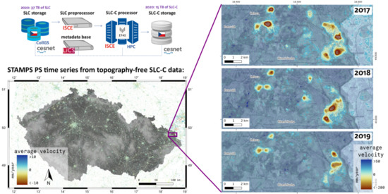
2. InSAR Functionality Implemented within IT4S1

The IT4S1 system architecture consists of three levels, an SLC data pre-processor (see Section 2.1) that generates SLCC data, an InSAR/MT-InSAR processor (see Section 2.2) and a post-processing that includes a basic visualisation part described in Section 2.3, for the purposes of this article. The modules are interrelated as shown in Figure 2.

2.1. Generation of SLC-C Data

The generation of the SLCC ARD is the core part of the IT4S1 system architecture. It connects storage centres of Sentinel-1 SLC data (at CollGS) and of final processed SLCC data. A metadata database system (a metadata base) and SLC preprocessor are two separate servers. An HPC facility was used for the main SLCC processing (and later for their InSAR processing), see Figure 2.
After the ingestion of a new Sentinel-1 SLC acquisition to CollGS, a metadata database system solution transferred from LiCSAR [17] ensures a proper identification of its bursts including information about their geographic coverage. When activated, the SLC preprocessor loads the SLC data with the latest available ephemeris data and splits it into bursts. The SLC preprocessor is using current calibration auxiliary data for Sentinel-1 satellites and the latest ephemeris data for further usage. The high quality Precise Orbit Determination (POD) ephemeris are available 21 days after the Sentinel-1 data acquisition, however ISCE processing routines allow a lower quality on-board ephemeris with no significant loss of performance in further steps. Routines of ISCE [7] open-source InSAR processing package are run at the SLC preprocessor server and the preprocessed burst SLC images are uploaded to the SLCC processor (an IT4Innovations HPC facility).
At the SLCC processor HPC facility, a custom solution prepares coherent burst combinations in order to perform ESD computation and correction. At this stage, a chronologically preceding set of compatible SLCC burst images (already existing in the framework of the same relative orbit track, see Section 2.1.1) are linked to the processing chain as “primary” burst images. The newly arrived SLC image is recognised as a “secondary” image. The interferometric combinations between both primary and secondary bursts are extremely coherent due to the short temporal revisit time of Sentinel-1, therefore well applicable for ESD computation. Algorithms of ISCE are applied, performing the preprocessing of secondary bursts until the stage of generating range fine offset fields for every secondary burst. The fine offset field grids contain estimated non-displacement phase due to a stereoscopic effect of topography observed from two slightly different satellite positions at both primary and secondary bursts. In order to simulate this topographic phase, we apply an SRTM 1 arc-second digital elevation model (DEM) [19] to form a height-per-pixel image fitting the primary bursts during the initial step (Section 2.1.1). The range offset fields are removed from the secondary bursts and these are saved into an SLCC storage for further use. Such produced SLCC data are ready for a direct generation of a topography-free interferogram [20] by a simple operation of complex conjugate.

2.1.1. Establishing Base Dataset

As the first step, a systematic data storage environment is established, aiming for the data storage structure: RELORB/SWATH/BURST_TANX/YEAR, where RELORB is a relative orbital track number of Sentinel-1 satellites, SWATH is a number from 1–3 identifying one of the three Sentinel-1 swaths, BURST_TANX is a burst identifier based on a naming convention established by LiCSInfo approach of the LiCSAR system [17]. In order to avoid large number of files in BURST_TANX folder, we sort them in subfolder YEAR (year of acquisition date). Names of the SLCC files are in the form of YYYYMMDD.slc (e.g., 20200201.slc for an SLCC image from 1st February 2020).
We establish a base dataset for each RELORB/SWATH. Here, we manually select the primary SLC image, with the main condition to have a full burst coverage across the whole region of interest (across Czechia, in this case). The initial processing is performed by the original ISCE approach. Based on the acquisition metadata and automatically downloaded SRTM DEM, ISCE would generate files containing latitude, longitude, height and line of sight (LOS) angle values for every pixel in the reference SLC image. These files are modified and stored per burst, i.e., under the BURST_TANX subfolder, in a geom folder.

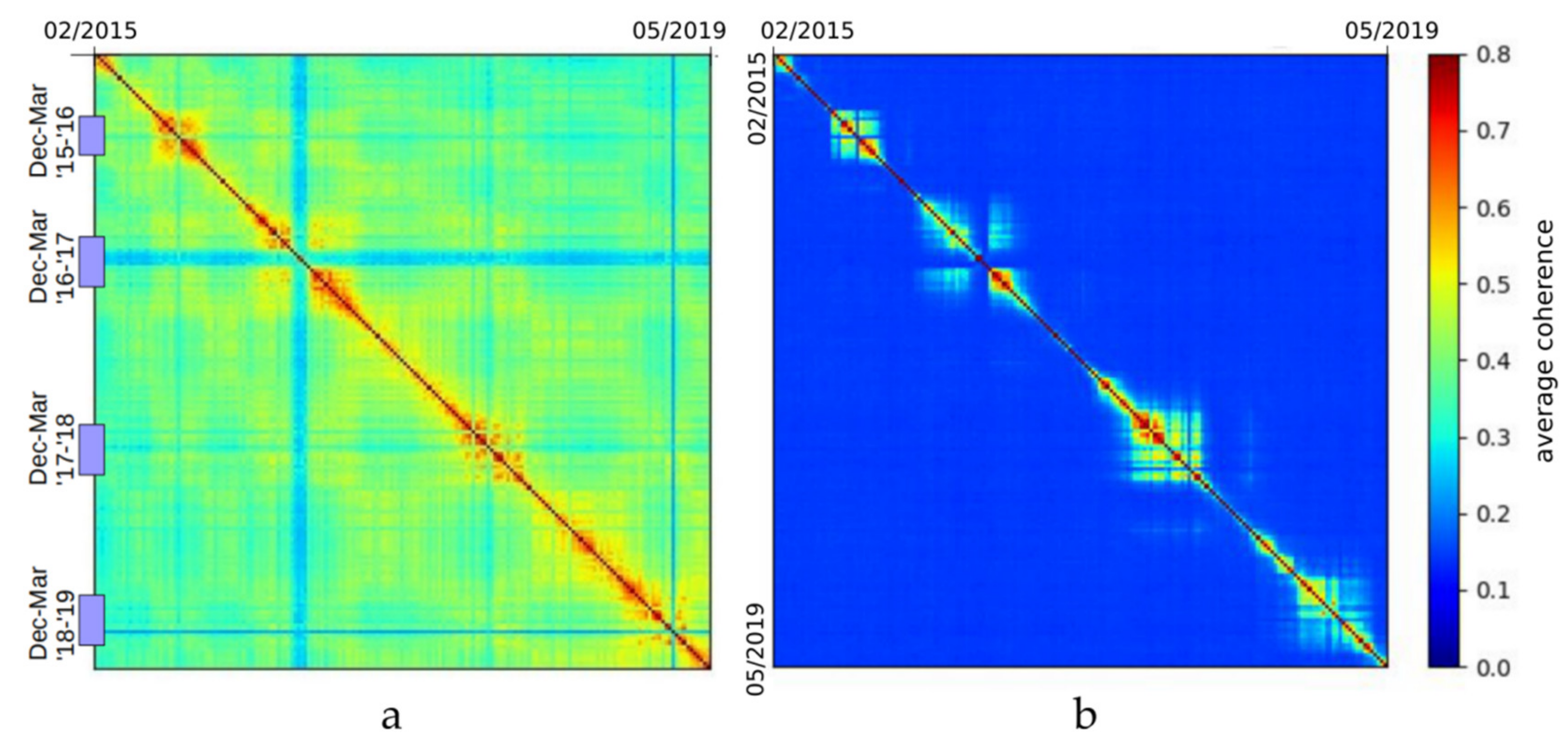
2.1.2. Coregistration Process

The coregistration process of a new acquisition A follows the original procedure as implemented by ISCE topsApp.py script [21], until the fineresamp step.
The existing geom data (containing lookup tables of 3-D geographic coordinates towards primary SLC data) are linked, rather than regenerated. In the case of other existing SLCC files in the database, a check is performed and the burst SLCC images of an acquisition B closest in time to the acquisition A data are linked as secondary reference data. The primary reference SLC data would be used to support the coregistration step by an amplitude cross-correlation, while the ESD estimation is performed towards the secondary reference data, not directly to the SLC data of the primary acquisition. As tested in [20] and shown in the results further on, we did not identify biases in any full resolution interferometric combination caused by this cascade approach, as the coregistration accuracy is anyway kept to the level of 0.001 pixel [22].
The key outputs of the ISCE topsApp.py coregistration approach, used as the basis for SLCC generation, are range and azimuth fine-offset files, correcting for a subpixel misregistration in the range and azimuth directions. These include both DEM-based height correction and the ESD-based correction and other refinements [21]. After the fineresamp step of topsApp.py, leading into a set of bursts resampled to the reference SLC, the resampled burst images I are deramped by a range fine offset file R. The azimuth fine offset file is neglected as (not considered significant). The deramping as the last step leading to burst SLCC files is performed according to Equation (1):
S L C C = I × exp j 4 π r λ R
where r is a pixel resolution in the range direction and λ the SAR carrier wavelength.
Afterwards, a topography-free interferogram can be formed simply by a complex conjugate between any two SLCC files. We have formed coherence matrices from 15,932 interferometric combinations of a selected burst ID 95_1_21244 from a period between February 2015 to May 2019, and plotted in Figure 3. The coherence matrices show a median coherence over small areas (~1000 pixels) representing different types of scattering classes-urban and agricultural land types. The matrices can be used as a quality measure, demonstrating the interferometric signal is coherent also in combinations of SLCC files in very distant temporal baselines, as in case of urban areas (Figure 3a). The effect of a signal decorrelation related probably to the presence of snow in winter months can be observed as drops of coherence. Selected agricultural area decorrelates especially in summer months (Figure 3b), as expected.

2.2. Multitemporal InSAR Processing

The IT4S1 system was primarily designed for an on-demand InSAR analysis to identify ground or structure displacements in a given area of interest (AOI). The system performs a burst-wise multitemporal InSAR (MT-InSAR) processing. If the area of interest is larger than the burst, the separate MT-InSAR results per burst can be merged afterwards, e.g., using points in their overlap area as a common reference (sub-sequent bursts overlap themselves within approx. 1.5 km along their common orbital track or between swaths). Cropping a burst towards AOI before the MT-InSAR processing is allowed—in such case, the system performs a small area processing using optimised parameters, more tolerant to the pixel phase stability. The parameters are optimised in relation to the scale of a selected area to process, but without taking temporal sampling into account. Currently different types of MT-InSAR implementations of PS and SB are available in the system The primary processing is based on STAMPS MT-InSAR algorithms [23] that will be described in more details.
Depending on the number of points to process and the size of the dataset, a typical burst was processed by the STAMPS PS InSAR approach within 24–48 core-hours (in case of 100 interferograms dataset, formed in connection to a common primary SLCC), while it can take 72–96 core-hours for STAMPS SB InSAR approach (in the case of the same SLCC dataset, this would consist of 400 interferograms formed by default for SB approach, combining data in 4 shortest temporal connections). We report that we experienced an increase of processing time when the MATLAB scripts of STAMPS (steps 1–4) were run through the open-source Octave environment.
The IT4S1 architecture allows an advantageous use of an on-demand processing of a selected AOI. A script it4s1_process_all.sh would take latitude, longitude as coordinates for the centre point and radius of interest in kilometres, as basic parameters. Connected to burst metadata database, the script would identify bursts covering the AOI and would select overlapping bursts and generate their interferograms, in combinations set up based on requested processing method. These interferograms are generated in radar coordinates, either within the full burst, or cropped to the selected extents.
As outputs of requested processing methods (STAMPS PS only by default), the system generates comma-separated text (CSV) files per burst ID, containing computed measures such as a mean velocity rate, temporal coherence, estimated deformation value per image date and other parameters (e.g., standard deviation of the estimated velocity). Optional processing parameters include start and end dates, other processing techniques to be applied and a reference area.
Processing parameters for STAMPS algorithms are scaled automatically regarding the size of the selected area. An overview of selected parameters and their use is shown in Table 2, the explanation of the parameters can be found in [24]. The parameters drive several key components of STAMPS during its selection of pixels to be processed, estimation of non-deformation signal and the final inversion to the deformation time series. We keep the parameters oriented to indicate deformation in a small to moderate scale (e.g., we remove long wavelength deformation through a deramping over whole region, using parameter scla_deramp).
The processing chain starts by clipping the dataset to smaller data patches that are processed in parallel (one patch per processing core). Within each patch, we select pixel candidates based on amplitude dispersion index (ADI) [23] computed from interferogram magnitude images. Afterwards, we run STAMPS steps [24] 1, 2 (read data and estimate phase noise for them) and step 4 (dropping pixels based on their noise standard deviation, weed_standard_dev); the step 3 (selection of pixels based on their spatial consistence) is skipped. We report possibility of a direct use of Octave to run the STAMPS scripts for the steps 1–4.
We then merge the patches through STAMPS step 5 (and merge them to a grid of resolution merge_resample_size). Next steps 6 (3-D phase unwrapping) and 7 (estimation of a spatially-correlated look angle error, including correction of phase induced through atmosphere) iterate. In total, 6 iterations are performed, refining the error terms to improve the estimation of unwrapped phases (step 6). Almost every iteration includes a specific optimisation to select the input set of interferograms (based on their noise standard deviation ifg_std computed by ps_calc_ifg_std), perform atmospheric phase correction, (optionally) 2-D deramping of the overall spatial phase ramp, etc. Finally, a custom approach is used to compute the standard deviation and temporal coherence of the output estimates [20,25].
Additionally, the data generated for STAMPS processing were optionally used for reprocessing using other algorithms implemented within the system—an octave-based SALSIT PS software [20] and a python-based LiCSBAS software [26]. These tools were considered complementary at the moment and are not included to the automatic processing chain (they are briefly discussed in the following subsections).

2.2.1. Primary Processing by PS InSAR

The STAMPS PS approach starts from a dataset of wrapped differential interferogram images. Since the phase offsets due to topography were already removed in SLCC images, the generation of a burst-wise differential interferogram without spatial filtering is performed rapidly within 8 s per one computing core. Afterwards, the ADI is calculated using magnitude of formed interferograms, rather than of the backscatter intensity values extracted from original SLC images as used by original STAMPS PS routine [23].
The process of interferogram generation is parallelised using Parallel tool [27], in order to split processing of interferograms to available computing cores. STAMPS MT-InSAR algorithms have been parallelised in a similar manner - the processing splits the whole area into patches that are processed in parallel. The processed data are merged for the last STAMPS steps - the unwrapping and estimation of so-called spatially correlated look angle error (SCLA). These last steps are performed fast. They form an iterative process using different settings per each iterative run - these settings regulate the number (and quality) of interferograms used to estimate SCLA, optionally remove atmospheric phase correlated with DEM and remove an overall 2-D phase ramp if it appears within the whole area.
After processing using STAMPS PS method, the same formed dataset can be assessed by the SALSIT PS InSAR tool [20]. SALSIT is an Octave-based open-source PS processor targeting infrastructure monitoring tasks [9,28], and providing evaluation of a geodetic quality of measurements. Both implementations showed similar outputs [28], but SALSIT parameters were set to include as many PS points as possible, while a reduction of the point density was used within the STAMPS PS approach.

2.2.2. STAMPS SB and Quasi-SB Processing

The full STAMPS processing chain merges results of both PS and SB techniques [23]. We keep outputs of both processing techniques separate in order to allow for comparison of results. For STAMPS SB MT-InSAR, we form the network of SB interferograms in the fashion of combining each SLCC image with four following dates, as described by the authors of [17]. The estimated deformation values are inverted toward the same reference date as used for STAMPS PS. We use a standard processing chain [23], with parameters optimised in a manner described in Section 2.2 that allows for processing of more points than in the case of PS, while avoiding biases that would have been induced by points affected by decorrelation.
As a seasonal snow is common in Czechia, it is often not desirable to use winter acquisitions to form interferograms for the MT-InSAR time series inversion. Similarly, dense vegetation tends to decorrelate SAR signals fast during warm seasons. In order to improve the STAMPS SB results and allow for the identification of more points in the InSAR time series, the IT4S1 includes a custom workaround, named quasi-SB.
Within the quasi-SB approach, the formed SB interferograms are analysed for their overall (a median) spatial coherence values. A threshold for the median coherence is used to select interferograms that should be processed further. In case of losing the consistency of such subset (the dataset should be interconnected), new interferometric connections are generated to provide the necessary link to the STAMPS SB algorithm. The ADI is recalculated from the new subset of quasi-SB interferograms, leading to an increased number of SB candidate pixels for a reprocessing by STAMPS SB routine.
The effect is demonstrated in the area of Sokolov open pit mine [29], in Figure 4. Here, the average coherence threshold of 0.4 has been applied for a quasi-SB approach, leading to an increased number of evaluated SB points. The increased density of points within a subset of interferograms having a reasonable coherence also improves the 3-D phase unwrapping. On the other hand, a signal related to a deformation occurring during the masked temporal periods is not monitored.

2.2.3. LiCSBAS Processing

We have recently implemented LiCSBAS software [26] to IT4S1. This tool uses unwrapped interferograms into a specific NSBAS time series inversion [30]. We use the same interferograms generated in the SB network, filter them spatially using a Goldstein technique as implemented in Doris [31], multilook them in 10/2 pixels ratio (range/azimuth SAR direction, the final resolution of a pixel is ~26.5 m) and perform coherence-weighted unwrapping using snaphu [32]. We have integrated a basic improvement of this unwrapping problem [33], based on masking low coherent pixels (on coherence threshold 0.35) and using a nearest neighbour interpolation between kept pixels [33], in order to prevent unwrapping errors due to propagation of unwrapping window through noisy areas.
At this moment, we use this technique as complementary, since the phase unwrapping of full InSAR scenes are often biased by decorrelating factors, especially due to the dense vegetation cover in Czechia. We provide a brief example output of LiCSBAS processing further in Section 3.2.

2.3. Visualization of Results

In the current version of IT4S1, the results from MT-InSAR are exported into a comma-delimited text file (CSV) in order to import to a GIS interface. The CSV includes estimated LOS displacement values per each date, linear velocity estimate, estimate of a residual height of the pixel, geographic coordinates in WGS-84 system, temporal coherence and a standard deviation of the velocity estimate based on [20].
For the purposes of visualising and demonstrating mean velocity maps, we have used GDAL [34] to rasterise all processed outputs per burst into 0.001° resolution images, recompute their mean velocity values (in mm/year) to vertical direction w.r.t. their average incidence angle (see Table 1) and rounded to the nearest integer, merge and spatially smooth using cubic spline function and export to a simple web map: http://seth4.ics.muni.cz/lazecky.
For plotting of time series figures for a selected point we currently use a custom giSAR toolbox [35] developed for Quantum GIS (currently for version 2.x only). An example of a PS processing result over Ostrava-Karvina undermined region in Figure 5 displays time series of a selected point on top of the downsampled velocity raster, from the Quantum GIS+giSAR toolbox environment. A modified version of open plugin “PS Time Series Viewer” [36] is used within the giSAR tool. The future development counts with updating the structures towards use of NetCDF format for further data sharing and visualisation using modern tools.
The time series plot also demonstrates the ability of the system to capture relatively fast non-linear displacements. This was achieved mainly by specifically optimised parameters for STAMPS PS processing, with the key parameter being unwrap_time that can be established shorter in case of Sentinel-1 data, thanks to its high revisit frequency. In this case, manually selected unwrap_time = 8 resulted in the least number of temporal phase unwrapping errors that would be otherwise present due to fast and non-linear terrain deformation causing phase jumps.

3. Processing over Czech Bursts

The IT4S1 system stores Sentinel-1 SLCC data burst-wise. It is a dataset ready for direct application of time series processing techniques on a burst-wise level, or on burst subsets. This section provides an overview on the full nation-wide PS product created by a simple merge of estimated LOS velocities generated per each burst in the late 2017 (Section 3.1). Section 3.2 provides an example of on-demand processing tasks performed on burst subsets using the current SLCC dataset, over an active mining area.
Further examples of application of the on-demand processing outputs of IT4S1 over Czech areas were documented in our previous works, further works are anticipated as well. In the case of an underground gas storage facility in the Tvrdonice area, seasonal deformations were identified and their correlation to the gas reservoir processes was studied in [37]—there we identify a change of the seasonal deformations behaviour behind a tectonic fault. Earlier, we have attempted to identify slope instabilities around Ostravice [29], concluding about unreliability of both PS and SB outputs in the area of dense vegetation for detection of slow slope instabilities.

3.1. Nationwide Processing Output of Czechia

The nation-wide processing of the whole Czechia has been performed in the end of 2017. The whole SLCC dataset of 352 bursts were processed using STAMPS PS, having each between 90–120 SLCC images per burst (total data of ~10 TB). In total, 8856 core-hours were reserved for the processing, while the real processing time was 3559 core-hours. The processing resulted in around 15 million PS points.
Most of Czech areas are covered by two descending and two ascending tracks. This would allow for an advanced analysis, computing horizontal and vertical motion vectors from the varying LOS observations [18]. However, in this test, only a simple merge was performed - mean velocity estimates were simply averaged and resampled into ~100 × 100 m resolution (0.001° in WGS-84) burst-wise GeoTIFF raster files, and merged to form a global map of (mainly vertical) mean displacement velocity over Czechia, valid for the covered period between 10/2014-09/2017. As the displacements in Czechia are of a local scale, it was not necessary to incorporate correction on varying reference areas - we have used the default STAMPS referencing based on the average overall estimated values (we used a median instead of mean value). We present the output in Figure 6.
As it can be observed from Figure 6, there are only few (urban) areas in Czechia demonstrating a noticeable linear trend of displacements. These are or should be subject to a separate investigation. The areas denoted S and O identify terrain deformation over previously presented locations—the open pit mine area in Sokolov surroundings (Figure 4) and a subsidence related to black coal mining in the Ostrava-Karvina region, covered by Figure 5.
We provide several other examples in Figure 7, by zooming into the map. These are capturing following deformations that can be of a particular interest for further works:
-
Deformations in the surroundings of an open pit mine near Polish Turów (Figure 7b). Subsidence of a German Zittau and the border area between Czechia and Germany was observed as well;
-
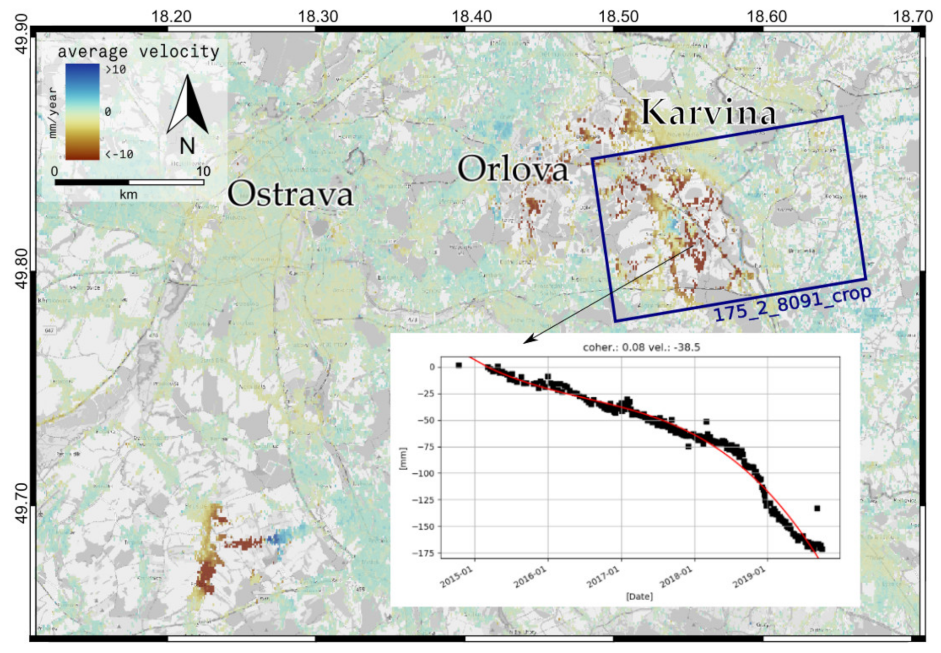
Subsidence and uplift detected over an active black coal mine in the Brusperk vicinity (Figure 7c);
-
Settlement of an industrial area in Prostejov city (Figure 7d);
-
Uplift in the surroundings of Kladno city (Figure 7e);
-
Local subsidence or a building settlement in the surroundings of Hostivice (Figure 7f).

3.2. Small Area On-Demand Processing—CSM Mine Example

As the PS technique is limited for monitoring areas with a lack of objects with a stable radar backscatter over time, we apply also the STAMPS SB technique in order to increase the number and density of measurement points. The use of SLCC data allows a fast generation of interferograms according to any custom defined graph of interferometric connections. In our current standard SB approach, we form four connections per an SLCC epoch into the SB graph. The additional filtering and phase unwrapping operations are performed within STAMPS SB algorithms only on an interconnected selection of points having ADI > 0.52 (see Table 2). This approach avoids biasing by decorrelated pixels, such as of densely vegetated areas, but may lead to phase unwrapping errors in moderately vegetated areas affected by a strong deformation signal. We experience this problem in the case of subsidence monitoring in non-urban areas due to an active underground mining, e.g., in Karvina region, demonstrated on a preliminary study of an active CSM Mine.
We selected an 8 × 8 km area in the Karvina region undermined by an active black coal CSM Mine as an example demonstrating the on-demand processing routine. We ran an automated processing using both STAMPS PS and SB techniques with optimised small area parameters (Table 2) and focused on a crop from a single burst 175_2_8091. For this particular burst, we used the current SLCC dataset of 220 SLCC images covering period of February 2015–September 2019. Both techniques finished the burst crop processing within 2 reserved node-hours (48 core-hours).
Differences in the deformation estimated by the automatic STAMPS PS and SB can be observed in Figure 8a,b. The time series inversion by PS is accurate for stably reflecting objects, already for a small number of temporal samples [1,25]. The increased density of points within coherent areas of SB network interferograms allows the estimation of deformations of a larger magnitude [3,23].
Additionally, we also include a preview of the output by LiCSBAS algorithm [26] applied to the same graph of SB connections, in Figure 8c. Here, we estimate LOS velocity rates over all unwrapped pixels in the area, including densely vegetated areas (covering most of the scene). While the subsiding areas were identified correctly with the estimated velocity rates corresponding to the STAMPS outputs, the vegetated zones (skipped by the STAMPS selective approach) are evaluated as strongly subsiding in less likely rates. As the vegetation-related phase (including moisture changes) can bias the unwrapping process [38] and should be solved in future, we consider the LiCSBAS output preliminary at the moment.
The possibility of significant differences in relation to the selected processing technique demands a careful interpretation of the results. Further investigation (outside the scope of this article) should include combination of other bursts overlapping the AOI from different tracks [18]. In this example, we compared STAMPS PS, STAMPS SB and LiCSBAS NSBAS outputs of the 175_2_8091 burst to levelling measurements available in the area. The original precise levelling of points over the subsiding area was connected to a reference point outside the area (in >4 km distance). The measurement instrument DNA 03 Leica has mean kilometric error of 0.3 mm/km. Mean kilometric errors of measured and corrected height from the precise levelling ranged between 0.6–1.6 mm/km. The accuracy of differences of the measurements was evaluated in the principle of the law of accumulation of errors. The mean error of the height differences within each levelling measurement ranged between 0.8–2.3 mm. For the double-difference using one of the levelling points as reference (depicted in Figure 8) toward the levelling point of interest (POI), the mean levelling errors were calculated as 1.9–2.8 mm.
All STAMPS and LiCSBAS results were referenced to a pixel closest to a selected levelling point and to a similar starting date (beginning of April 2015). Their output LOS estimates dLOS were recomputed to the vertical direction dU in a simplified manner (see Equation (2)), and plotted in Figure 8d as (STAMPS) PS-U, SB-U and LiCSBAS-U, together with corresponding differences of levelling measurements.
d U = d L O S c o s θ i n c
where θinc is the mean LOS incidence angle of the SAR measurement.
The general deformation trends estimated by MT-InSAR correspond to the levelling, yet we observe significant differences within each temporal epoch of up to a centimetre (see Figure 8d). This can be related to continuous local changes (rectification of rails and an embankment between rails) that affect objects in the close neighbourhood of the stabilised reference levelling point. We should note that the STAMPS PS and SB reference points differ from the exact levelling point. Instead, they represent an object having a dominant and stable radar response (in case of PS), or a cluster of scatterers contributing to the merged phase signal within a spatially filtered SB pixel (downsampled to 50 × 50 m, see Table 2).

4. Discussion

Using the framework of continuously updating SLCC images ready for advanced processing, the system leads not only to generate annual maps of terrain and urban displacements over the whole Czech country but also towards an innovative system for an early identification of risks due to identified displacements, e.g., in cases of critical infrastructure. Data from newly arrived images can be extracted directly for the selected PS or SB points where the system would perform an additional update analysis. Innovative static or dynamic InSAR-based outputs can be included to risk management systems but can be used also by local authorities, or scientific communities (e.g., in the field of geology or geodesy). Further major development of the system would allow for a more reliable detection of a slope motion under a vegetation cover, once long-wavelength SAR data become available, as expected from upcoming NISAR mission [39].
The modified/simplified ISCE-based coregistration into the form of SLCC images may be still affected by various biases, including variation in atmospheric delays on pixel level per image. We were notified that a slight misalignment, especially in slant range direction, may cause a shift in a subpixel level that may result in a decreased accuracy of full-resolution PS InSAR estimations performed afterward (email communication with Dr. P. Agram, May 2018). It is recommended to follow the original TOPS stacking approach [8]. We did not, however, experience significant noise in the SLCC dataset. Comparison of IT4S1 system with another existing solution, SARPROZ [4], proved its comparable accuracy in case of a Spanish Costa del Sol area [40]. Similarly, we demonstrated the quality of the processing outputs in the search of topographic residuals in a mountainous area in Spain, and within a coherence analysis of SARPROZ and IT4S1 (STAMPS and SALSIT) in [20]. With the confidence on the phase signal quality in SLCC data, we demonstrated the applicability of the system on infrastructure monitoring outside of Czechia, in the case of the La Vinuela dam in Spain [28] and a deforming terrain in El Salvador [41]. This also demonstrates a possibility of the application of deployed IT4S1 system to areas outside of designated region of interest, though it is not the primary objective of the system (technical issues should be expected in case of extended areas covering the same relative orbit/swath configuration).
The IT4S1 system currently works only with copolarised Sentinel-1 data. Once the coregistering equations are solved, they can be applied to coregister also cross-polarised SLC data. The cross-polarised signal would be used for intensity/amplitude-based applications, as a detection of deforestation [42] or other forest/vegetation changes [43], etc. The amplitude exploitation would allow for other change detection applications of SAR data, such as monitoring soil moisture changes, identification of flooded areas, studying urban growth and other topics [44]. The system should include cross-polarisation data structures in its future version, aiming toward preparation for ingesting data from future satellite SAR missions, e.g. aforementioned NISAR. Though IT4S1 was prepared specifically for a systematic processing of Sentinel-1 data, it can be further developed to ingest also data from other SAR satellites.

4.1. Computational Load

In order to perform the ESD correction in the SLCC generation phase, the system extracts all available bursts in a related swath overlapping Czechia within a current date, and registers them to already preprocessed reference bursts. The generation of one SLCC epoch is performed for approx. 18–20 bursts (per swath) at once. We use a 24-core computing node for this generation of SLCC data and we report an average rate of 2.2 min per burst (this includes some non-parallelised parts of the processing chain).
The whole Czechia is segmented by 370 burst units. Currently, we generate and store SLCC data for 352 bursts. We report the current and expected computational load for generation of SLCC burst images over Czechia as:
-
until October 2017: 62,900 burst images; approximately 53,000 core-hours,
-
October 2017 to December 2020: approximately 136,000 burst images; approximately 61,000 core-hours.
The IT4S1 approach expects monthly allocation of 1700 core-hours for keeping the SLCC database over Czechia to date.
Thanks to the pre-processed data, the MT-InSAR processing itself is a lower computational burden. We currently reach a PS output of a full burst within 24–48 core-hours using the adapted STAMPS PS MT-InSAR. The generation of STAMPS SB results can take a larger amount of time, e.g., 48–72 core-hours per burst or more. In theory, time series approaches that consider only temporal signature of the data stack would compute the solution in a couple of minutes from such dataset, e.g., PS solution as implemented in SARPROZ, or other tools.
A spatially unfiltered interferogram of one burst (combination of two SLCC images) is generated within 8 s. A monthly update of the MT-InSAR results (using up to five new images for the six-day revisit time of Sentinel-1) is expected to take around 5 min per burst, meaning up to approximately 1400 core-hours monthly for the update of Czechia displacements in the case of a potential nationwide monitoring system.

4.2. Current and Future Storage Needs for Czechia

Sentinel-1 data cover the whole Czechia from 9 tracks, yielding approximately 180 new images per month. One image contains 24 bursts (8 bursts per 3 swath units), covering approximately 90 × 20 km area each with its LOS direction pixel spacing of approximately 3 × 14 m [45], and is distributed in files of a size around 4.5 GB in its compressed form, i.e., approx. 200 MB/burst in the compressed form and around 550 MB uncompressed (including both copolarised and cross-polarised image). For InSAR, only copolarised images are needed. We stored our generated SLCC burst images compressed to approximately 200 MB/burst.
In October 2017, 3580 unique Sentinel-1 SLC zip files covering Czechia were stored in CollGS (~15.7 TB), while the expected number of images in December 2020 is 7740 SLC files (~34 TB). The full dataset of SLCC images consisted of ~8 TB in October 2017, the expected amount in December 2020 is less than 21 TB. The current monthly data size increment for Czech bursts is ~360 GB/month.

5. Conclusions

The IT4S1 system is an HPC-deployable solution based on open-source technologies. Whereas common HPC approaches of utilising Sentinel-1 images for InSAR start their processing chain from either original SLC data or raw non-coregistered data [46], the IT4S1 system allowed a faster and more flexible multitemporal processing thanks to availability of specifically pre-processed SLCC ARD images, based on ISCE/ISCE2 [7,8]. As these ARD already do not contain most of the phase induced by topography, Earth curvature, etc., there is no need to simulate and remove the topography and orbital ramp components per each generated interferogram, as typically done in other InSAR-oriented systems, e.g., LiCSAR [17]. The SLCC ARD proved its quality and effectivity to be used for a typical InSAR processing toward deformation monitoring. Yet we recommend using the original stacking approach [8] in order to keep high precision of the corrections.
The presented IT4S1 solution is available at https://code.it4i.cz/laz048/it4s1, and can be deployed in an HPC environment, given the pre-existing database of burst definitions [17] over a region of interest. It allows for an easy and effective inclusion of various MT-InSAR algorithms. The system is already capable of PS and SB through STAMPS [23] and SALSIT [20], as well as (experimentally) NSBAS time series through LiCSBAS [26]. A working MATLAB software is a prerequisite for IT4S1, as only a part of STAMPS scripts can be run through Octave directly. The IT4S1 system was designed to use a PBS job scheduler (qsub command). The job running commands can be modified prior to deployment to a system using another scheduler or, e.g., a cloud environment. The SLCC approach is suitable for inclusion of other advanced techniques, such as PS implementation of SARPROZ [4,47], experimental SqueeSAR [48] or a phase triangulation stacking [49]. It demonstrates a great advantage of ARD data generated in this form [8] for multitemporal analyses.
The SLCC ARD data can be generated using SAR processing tools that allow the computation of range pixel offsets. A further investigation may confirm whether the complex ESD operation can be substituted by a simple burst-based removal of an overall 2-D polynomial interferometric ramp. The ESD correction may be also fully skipped for the burst-wise processing, as the high accuracy of Sentinel-1 precise orbital data should satisfy needs of a purely geometric registration by simulating antenna steering to model the azimuthal ramp [50,51].
We presented the processing outputs of our customised STAMPS PS approach on all pre-processed bursts covering Czechia until autumn 2017. The large spatial coverage of Sentinel-1 InSAR brings advantages over in situ technologies, such as GNSS or other geodetic instruments, yet the character of MT-InSAR processing demands a careful interpretation of its output estimations.
The system and its results can find application for national geologic, urban planning, forestry or risk management applications, as, e.g., Floreon+ developed by IT4Innovations to support local risk management [52]. The IT4S1 could be further developed in this framework in a direction toward an automatic InSAR-based system that would make it possible to provide an early warning by detecting displacements around critical AOIs based on change analyses in interferometric time series. Although the Floreon+ system offers a web GIS environment, we kept the current outputs publicly available only in its simplified web map: http://seth4.ics.muni.cz/lazecky. A part of the processing is to be included to the Floreon+ webmap: https://floreon.eu/mapa.

Author Contributions

Writing—original draft preparation, conceptualization, methodology and software M.L.; software M.L., I.H., P.J.G., E.H., F.D.; Investigation, M.L., E.J.; funding acquisition and resources, J.M., Z.Š. All authors have read and agreed to the published version of the manuscript.

Funding

This work was supported by The Ministry of Education, Youth and Sports from the National Programme of Sustainability (NPU II) project “IT4Innovations excellence in science—LQ1602” and from the Large Infrastructures for Research, Experimental Development and Innovations project “IT4Innovations National Supercomputing Center—LM2015070”.

Acknowledgments

Access to computing and storage facilities owned by parties and projects contributing to the National Grid Infrastructure MetaCentrum, provided under the programme “Projects of Large Infrastructure for Research, Development, and Innovations” (LM2010005), is greatly appreciated. The author wishes to thank supportive colleagues from IT4Innovations and CESNET. The work is based on open-source technologies, the main processors being ISCE/ISCE2 by NASA/JPL and STAMPS-MTI. The LiCSInfo metadata database of Sentinel-1 images has been kindly offered by University of Leeds team in 2016.

Conflicts of Interest

The authors declare no conflict of interest.

References

  1. Ferretti, A.; Prati, C.; Rocca, F. Nonlinear subsidence rate estimation using Permanent Scatterers in differential SAR interferometry. IEEE Trans. Geosci. Remote Sens. 2000, 38, 2202–2212. [Google Scholar] [CrossRef] [Green Version]
  2. Ferretti, A.; Savio, G.; Barzaghi, R.; Borghi, A.; Musazzi, S.; Novali, F.; Prati, C.; Rocca, F. Submillimeter Accuracy of InSAR Time Series: Experimental Validation. IEEE Trans. Geosci. Remote Sens. 2007, 45, 1142–1153. [Google Scholar] [CrossRef]
  3. Berardino, P.; Fornaro, G.; Lanari, R.; Sansosti, E. A new algorithm for surface deformation monitoring based on small baseline differential SAR interferograms. IEEE Trans. Geosci. Remote Sens. 2002, 40, 2375–2383. [Google Scholar] [CrossRef] [Green Version]
  4. Perissin, D.; Wang, T. Repeat-pass SAR Interferometry with Partially Coherent Targets. IEEE Trans. Geosci. Remote Sens. 2012, 50, 271–280. [Google Scholar] [CrossRef]
  5. De Zan, F.; Guarnieri, A.M. TOPSAR: Terrain observation by progressive scans. IEEE Trans. Geosci. Remote Sens. 2006, 44, 2352–2360. [Google Scholar] [CrossRef]
  6. Yague-Martinez, N.; Prats-Iraola, P.; Gonzalez, F.; Brcic, R.; Shau, R.; Geudtner, D.; Eineder, M.; Bamler, R. Interferometric Processing of Sentinel-1 TOPS Data. IEEE Trans. Geos. Remote Sens. 2016, 54, 2220–2234. [Google Scholar] [CrossRef] [Green Version]
  7. Zebker, H.A.; Hensley, S.; Shanker, P.; Wortham, C. Geodetically Accurate InSAR Data Processor. IEEE Trans. Geosci. Remote Sens. 2010, 48, 4309–4321. [Google Scholar] [CrossRef]
  8. Fattahi, H.; Agram, P.; Simons, M. A network-based enhanced spectral diversity approach for TOPS time-series analysis. IEEE Trans. Geosci. Remote Sens. 2017, 55, 777–786. [Google Scholar] [CrossRef] [Green Version]
  9. Lazecky, M.; Bakon, M.; Hlavacova, I.; Sousa, J.J.; Real, N.; Perissin, D.; Patricio, G. Bridge Displacements Monitoring using Space-Borne SAR Interferometry. IEEE J. Sel. Top. Appl. Earth Obs. Rem. Sens. (J-STARS) 2016, 10, 205–210. [Google Scholar] [CrossRef] [Green Version]
  10. Lazecky, M.; Bakon, M.; Perissin, D.; Papco, J.; Gamse, S. Analysis of dam displacements by spaceborne SAR interferometry. In Proceedings of the ICOLD 2017, Prague, Czech Republic, 3–7 July 2017. [Google Scholar]
  11. Comut, F.C.; Ustun, A.; Lazecky, M.; Perissin, D. Capability of detecting rapid subsidence with Cosmo SkyMed and Sentinel-1 dataset over Konya city. In Proceedings of the ESA Living Planet Symposium, ESA SP740, Prague, Czech Republic, 9–13 May 2016. [Google Scholar]
  12. Jiránková, E.; Lazecký, M. Specifics in the formation of substituence through in the Karvina part of the Ostrava-Karvina coalfield with the use radar interferometry. Acta Geodyn. Geomater. 2016, 13, 263–269. [Google Scholar] [CrossRef]
  13. Lazecky, M.; Jirankova, E.; Kadlecik, P. Multitemporal monitoring of Karvina subsidence trough using Sentinel-1 and TerraSAR-X interferometry. Acta Geodyn. Geomater. 2017, 14, 53–59. [Google Scholar] [CrossRef] [Green Version]
  14. Lazecky, M.; Comut, F.C.; Nikolaeva, E.; Bakon, M.; Papco, J.; Ruiz-Armenteros, A.M.; Qin, Y.; Sousa, J.J.; Ondrejka, P. Potential of Sentinel-1A for nation-wide routine updates of active landslide maps. Int. Arch. Photogramm. Remote Sens. Spatial Inf. Sci. 2016, XLI, 775–781. [Google Scholar] [CrossRef]
  15. Lazecky, M.; Hlavacova, I.; Kocich, D. Czech System for exploitation of land dynamics using Copernicus Sentinel-1 data. In Proceedings of the GIS Ostrava 2017, Ostrava, Czech Republic, 22–24 March 2017. [Google Scholar] [CrossRef]
  16. Lazecky, M. System for Automatized Sentinel–1 Interferometric Monitoring. In Proceedings of the 2017 conference on Big Data from Space, Toulouse, France, 28–30 November 2017; pp. 161–165. [Google Scholar]
  17. Lazecký, M.; Spaans, K.; González, P.J.; Maghsoudi, Y.; Morishita, Y.; Albino, F.; Elliott, J.; Greenall, N.; Hatton, E.; Hooper, A.; et al. LiCSAR: An Automatic InSAR Tool for Measuring and Monitoring Tectonic and Volcanic Activity. Remote Sens. 2020, 12, 2430. [Google Scholar] [CrossRef]
  18. Wright, T.J.; Parsons, B.E.; Lu, Z. Toward mapping surface deformation in three dimensions using InSAR. Geophys. Res. Lett. 2004, 31, 1–5. [Google Scholar] [CrossRef] [Green Version]
  19. Farr, T.G.; Rosen, P.A.; Caro, E.; Crippen, R.; Duren, R.; Hensley, S.; Kobrick, M.; Paller, M.; Rodriguez, E.; Roth, L.; et al. The shuttle radar topography mission. Rev. Geophys. 2007, 45, 1–33. [Google Scholar] [CrossRef] [Green Version]
  20. Lazecky, M.; Hlavacova, I.; Martinovic, J.; Ruiz-Armenteros, A.M. Accuracy of Sentinel-1 interferometry monitoring system based on topography-free phase images. Procedia Comput. Sci. 2018, 138, 310–317. [Google Scholar] [CrossRef]
  21. ISCE Team, Overview of S1A TOPS Processing with ISCE –topsApp.py. Available online: http://etdedata.gein.noa.gr/ISCE_UNAVCO/topsApp_ISCE_20160418.pdf (accessed on 31 July 2020).
  22. Qin, Y.; Perissin, D.; Bai, J. Investigations on the coregistration of Sentinel-1 TOPS with the conventional cross-correlation technique. Remote Sens. 2018, 10, 1405. [Google Scholar] [CrossRef] [Green Version]
  23. Hooper, A. A multi-temporal InSAR method incorporating both persistent scatterer and small baseline approaches. Geophys. Res. Lett. 2008, 35, L16302. [Google Scholar] [CrossRef] [Green Version]
  24. Hooper, A.; Bekaert, D.; Hussain, E.; Spaans, K.; Arikaan, M. StaMPS/MTI Manual. Available online: https://github.com/dbekaert/StaMPS/blob/master/Manual/StaMPS_Manual.pdf (accessed on 20 February 2020).
  25. Colesanti, C.; Ferretti, A.; Novali, F.; Prati, C.; Rocca, F. SAR Monitoring of Progressive And Seasonal Ground Deformation Using the Permanent Scatterers Technique. IEEE Trans. Geosci. Remote Sens. 2003, 41, 1685–1701. [Google Scholar] [CrossRef] [Green Version]
  26. Morishita, Y.; Lazecky, M.; Wright, T.J.; Weiss, J.R.; Elliott, J.R.; Hooper, A. LiCSBAS: An Open-Source InSAR Time Series Analysis Package Integrated with the LiCSAR Automated Sentinel-1 InSAR Processor. Remote Sens. 2020, 12, 424. [Google Scholar] [CrossRef] [Green Version]
  27. Tange, O. GNU Parallel-The Command-Line Power Tool. USENIX Mag. 2011, 36, 42–47. [Google Scholar]
  28. Ruiz-Armenteros, A.M.; Lazecky, M.; Hlavacova, I.; Bakon, M.; Delgado, J.M.; Sousa, J.J.; Lamas-Fernández, F.; Marchamalo, M.; Caro-Cuenca, M.; Papco, J.; et al. Deformation monitoring of dam infrastructures via spaceborne MT-InSAR: The case of La Viñuela (Málaga, southern Spain). Procedia Comput. Sci. 2018, 138, 346–353. [Google Scholar] [CrossRef]
  29. Lazecky, M. Identification of active slope motion in Czech environment using Sentinel-1 interferometry. Springer Lect. Notes Geoinf. Cartogr. 2018, 1, 21–23. [Google Scholar]
  30. Schmidt, D.A.; Bürgmann, R. Time-dependent land uplift and subsidence in the Santa Clara valley, California, from a large interferometric synthetic aperture radar data set. J. Geophys. Res. Solid Earth 2003, 108, 2267. [Google Scholar] [CrossRef] [Green Version]
  31. Kampes, B.; Hanssen, R.F.; Perski, Z. Radar Interferometry with Public Domain Tools. In Proceedings of the Fringe 2003, Frascati, Italy, 1–5 December 2003. [Google Scholar]
  32. Chen, C.W.; Zebker, H.A. Phase unwrapping for large SAR interferograms: Statistical segmentation and generalized network models. IEEE Trans. Geosci. Remote Sens. 2002, 40, 1709–1719. [Google Scholar] [CrossRef] [Green Version]
  33. Chen, C.W.; Zebker, H.A. Network approaches to two-dimensional phase unwrapping: Intractability and two new algorithms. J. Opt. Soc. Am. 2000, 17, 401–414. [Google Scholar] [CrossRef]
  34. GDAL/OGR Geospatial Data Abstraction Software Library. Available online: https://gdal.org (accessed on 31 July 2020).
  35. giSAR (Quantum GIS Toolbox). Available online: https://github.com/espiritocz/giSAR (accessed on 20 February 2020).
  36. Sucameli, G. PS Time Series Viewer. Available online: https://gitlab.com/faunalia/ps-speed (accessed on 25 August 2020).
  37. Rapant, P.; Struhar, J.; Lazecky, M. Radar Interferometry as a Comprehensive Tool for Monitoring the Fault Activity in the Vicinity of Underground Gas Storage Facilities. Remote Sens. 2020, 12, 271. [Google Scholar] [CrossRef] [Green Version]
  38. Ansari, H.; De Zan, F.; Parizzi, A. Study of Systematic Bias in Measuring Surface Deformation with SAR Interferometry. IEEE Trans. Geosci. Remote Sens. 2020, 27, 10061. [Google Scholar] [CrossRef]
  39. Overview of NISAR Mission and Airborne L & S SAR. Available online: https://vedas.sac.gov.in/vedas/downloads/ertd/SAR/L_1.pdf (accessed on 25 May 2020).
  40. Ruiz-Armenteros, A.M.; Lazecky, M.; Ruiz-Constán, A.; Bakon, M.; Delgado, J.M.; Sousa, J.J.; Galindo-Zaldívar, J.; de Galdeano, C.S.; Caro-Cuenca, M.; Martos-Rosillo, S.; et al. Monitoring continuous subsidence in the Costa del Sol (Málaga province, southern Spanish coast) using ERS-1/2, Envisat, and Sentinel-1A/B SAR interferometry. Procedia Comput. Sci. 2018, 138, 354–361. [Google Scholar] [CrossRef]
  41. Chavez Hernandez, J.A.; Lazecky, M.; Sebesta, J.; Bakon, M. Relation between surface dynamics and remote sensor InSAR results over the Metropolitan Area of San Salvador. Nat. Hazards 2020, 103, 3661–3682. [Google Scholar] [CrossRef]
  42. Lazecky, M.; Lhota, S.; Wenglarzyova, P.; Joshi, N. Evaluation of forest loss in Balikpapan Bay in the end of 2015 based on Sentinel-1A polarimetric analysis. In Proceedings of the IGRSM 2018, Kuala Lumpur, Malaysia, 24–25 April 2018. [Google Scholar] [CrossRef] [Green Version]
  43. Lazecky, M.; Wadhwa, S.; Mlcousek, M. Simple method for identification of forest windthrows from Sentinel-1 SAR data incorporating PCA. In Proceedings of the CENTERIS SARWatch 2020, Vilamoura, Portugal, 21–23 October 2020. accepted for publication. [Google Scholar]
  44. Nielsen, A.A.; Canty, M.J.; Skriver, H.; Conradsen, K. Change detection in multi-temporal dual polarization Sentinel-1 data. In Proceedings of the 2017 IEEE International Geoscience and Remote Sensing Symposium (IGARSS), Fort Worth, TX, USA, 23–28 July 2017. [Google Scholar] [CrossRef]
  45. Bourbigot, M.; Johnsen, H.; Piantanida, R.; Hajduch, G.; Poullaouec, J. Sentinel-1 Product Definition, Technical Report Ref. S1-RS-MDA-52-7440. Available online: https://sentinel.esa.int/documents/247904/1877131/Sentinel-1-Product-Definition (accessed on 20 February 2020).
  46. De Luca, C.; Zinno, I.; Manunta, M.; Lanari, R.; Casu, F. Large areas surface deformation analysis through a cloud computing P-SBAS approach for massive processing of DInSAR time series. Remote Sens. Environ. 2017, 202, 3–17. [Google Scholar] [CrossRef]
  47. Bakon, M.; Czikhardt, R.; Papco, J.; Barlak, J.; Rovnak, M.; Adamisin, P.; Perissin, D. remotIO: A Sentinel-1 Multi-Temporal InSAR Infrastructure Monitoring Service with Automatic Updates and Data Mining Capabilities. Remote Sens. 2020, 12, 1892. [Google Scholar] [CrossRef]
  48. Ferretti, A.; Fumagalli, A.; Novali, F.; Prati, C.; Rocca, F.; Rucci, A. A New Algorithm for Processing Interferometric Data-Stacks: SqueeSAR. IEEE Trans. Geosci. Remote Sens. 2011, 49, 3460–3470. [Google Scholar] [CrossRef]
  49. Samiei-Esfahany, S.; Hanssen, R.F. New algorithm for InSAR stack phase triangulation using integer least squares estimation. In Proceedings of the 2013 IEEE International Geoscience and Remote Sensing Symposium-IGARSS, Melbourne, VIC, Australia, 21–26 July 2013; pp. 884–887. [Google Scholar] [CrossRef]
  50. Sandwell, D.; Mellors, R.; Tong, X.; Xu, X.; Wei, M.; Wessel, P. GMTSAR An InSAR Processing System Based on Generic Mapping Tools. Available online: https://topex.ucsd.edu/gmtsar/tar/GMTSAR_2ND_TEX.pdf (accessed on 31 July 2020).
  51. Miranda, N. Definition of the TOPS SLC Deramping Function for Products Generated by the S-1 IPF. Tech. Rep. Available online: https://earth.esa.int/documents/247904/1653442/Sentinel-1-TOPS-SLC_Deramping (accessed on 31 July 2020).
  52. Podhoranyi, M.; Veteska, P.; Szturcova, D.; Vojacek, L.; Portero, A. A web-based modelling and monitoring system based on coupling environmental models and hydrological-related data. J. Commun. 2017, 12, 340–346. [Google Scholar] [CrossRef]
Figure 1. Projected Sentinel-1 centre lines for IW2 swaths of (a) ascending pass and (b) descending pass relative orbital tracks covering Czechia. Arrows depict direction of the satellite during each pass. Rectangles are projected burst units distributed within one Single Look Complex (SLC) data file from relative orbit 146 (a) and 124 (b).
Remotesensing 12 02960 g001
Figure 2. Architecture of IT4S1 system modules generating Sentinel-1 burst SLC-corrected (SLC-C) data and their interferometric processing.
Remotesensing 12 02960 g002
Figure 3. Interferometric coherence matrices of burst ID 95_1_21244 (February 2015—May 2019) over (a) urban area and (b) agricultural area.
Remotesensing 12 02960 g003
Figure 4. Sokolov open pit mine area processed by IT4S1 approaches (burst ID 44_2_8161): (a) STAMPS Persistent Scatterers (PS), (b) standard STAMPS Small Baseline (SB) and (c) optimised STAMPS quasi-SB using coherence threshold of 0.4. Top subfigures show plot of applied interferometric combinations, the bottom subfigures show estimated mean line-of-sight (LOS) displacement velocity.
Remotesensing 12 02960 g004
Figure 5. Example of a time series of a selected PS point, visualised using giSAR Quantum GIS toolbox. The area marked as 175_2_8091_crop defines a reprocessed crop of interest described in Section 3.2.
Remotesensing 12 02960 g005
Figure 6. Nation-wide STAMPS PS processing output over Czechia, using IT4S1 system. Letters S, O indicate areas of Sokolov (Figure 4) and Ostrava (Figure 5).
Remotesensing 12 02960 g006
Figure 7. Examples of detected terrain deformations within the full-scale nationwide PS processing (Sentinel-1 data from October 2014–September 2017, processed by STAMPS PS through IT4S1 system): (a) Map overview localising zoomed-in areas in this figure, (b) subsidence in the surroundings of Turów, (c) subsidence and uplift due to mining activities in the Brusperk area, (d) settlement in the industrial zone of Prostejov, (e) uplift in the surroundings of Kladno, (f) local subsidence near Hostivice.
Remotesensing 12 02960 g007
Figure 8. Mean LOS velocity estimated from burst ID 175_2_8091 (220 SLCC images, February 2015–September 2019) using (a) STAMPS PS, (b) STAMPS SB, (c) LiCSBAS NSBAS; (d) comparison of measurements of point of interest (POI) from (ac) recomputed to vertical direction (U) and levelling measurements.
Remotesensing 12 02960 g008
Table 1. Coverage of Sentinel-1 data over Czechia (all except marked * are active within the processing by IT4S1).
Relative OrbitSwathNo. of BurstsIncidence Angle
descending tracks
22 *1 *18 *33.5°
2221839.0°
2231743.6°
5131743.7°
9511833.6°
9521839.0°
9531843.7°
12411833.5°
12421839.0°
12431743.7°
16811833.7°
ascending tracks
4421539.2°
4431843.8°
7311833.7°
7321839.1°
7331843.7°
14611833.7°
14621839.0°
14631743.7°
17511833.6°
17521739.1°
Table 2. Selected STAMPS multitemporal InSAR (MT-InSAR) parameters used within IT4S1 automatised processing chain.
ParameterBurst-Wise PSSmall Area PSSmall Area SB
ADI threshold0.40.40.52
gamma_max_iterations355
gamma_change_convergence0.010.010.04
clap_win328–64
(size dependent)
8–64
(size dependent)
clap_low_pass_wavelength800 m800 m600 m
max_topo_err25 m30 m15 m
weed_standard_dev1.41.51.0
merge_resample_size50 m-50 m
unwrap_time_win90 days30 days730 days
unwrap_gold_alpha0.750.40.8
unwrap_gold_n_win1688–32
(size dependent)
unwrap_grid_size320200200
ifg_std threshold (first iteration)554545
scla_derampyesonly areas > 10 kmonly areas > 7 km

