Article

Spatiotemporal Variations of City-Level Carbon Emissions in China during 2000–2017 Using Nighttime Light Data

1
Department of Land Management, Zhejiang University, Hangzhou 310058, China
2
Collaborative Innovation Center of Atmospheric Environment and Equipment Technology, Jiangsu Key Laboratory of Atmospheric Environment Monitoring and Pollution Control (AEMPC), Nanjing University of Information Science & Technology, Nanjing 210044, China
3
Shanghai Key Laboratory of Atmospheric Particle Pollution and Prevention (LAP3), Department of Environmental Science and Engineering, Fudan University, Shanghai 200433, China
4
Department of Urban and Environmental Sociology, Helmholtz Centre for Environmental Research-UFZ, Permoserstraße 15, D-04318 Leipzig, Germany
5
School of Life and Environmental Sciences, Schmid College of Science and Technology, Chapman University, One University Drive, Orange, CA 92866, USA
*
Author to whom correspondence should be addressed.
Remote Sens. 2020, 12(18), 2916; https://doi.org/10.3390/rs12182916
Submission received: 26 August 2020 / Revised: 4 September 2020 / Accepted: 7 September 2020 / Published: 8 September 2020

Abstract

:
China is one of the largest carbon emitting countries in the world. Numerous strategies have been considered by the Chinese government to mitigate carbon emissions in recent years. Accurate and timely estimation of spatiotemporal variations of city-level carbon emissions is of vital importance for planning of low-carbon strategies. For an assessment of the spatiotemporal variations of city-level carbon emissions in China during the periods 2000–2017, we used nighttime light data as a proxy from two sources: Defense Meteorological Satellite Program’s Operational Linescan System (DMSP-OLS) data and the Suomi National Polar-orbiting Partnership satellite’s Visible Infrared Imaging Radiometer Suite (NPP-VIIRS). The results show that cities with low carbon emissions are located in the western and central parts of China. In contrast, cities with high carbon emissions are mainly located in the Beijing-Tianjin-Hebei region (BTH) and Yangtze River Delta (YRD). Half of the cities of China have been making efforts to reduce carbon emissions since 2012, and regional disparities among cities are steadily decreasing. Two clusters of high-emission cities located in the BTH and YRD followed two different paths of carbon emissions owing to the diverse political status and pillar industries. We conclude that carbon emissions in China have undergone a transformation to decline, but a very slow balancing between the spatial pattern of high-emission versus low-emission regions in China can be presumed.

Graphical Abstract

1. Introduction

China is the largest carbon emitter in the world, contributing 30% of global carbon emissions [1], and is one of the most polluted countries. To address the climate change crisis, China submitted the Intended Nationally Determined Contributions (INDCs) to the United Nations, announcing that China will reach its peak carbon emissions and reduce its carbon intensity by 60% to 65% from 2005 levels in 2030 [2]. Under the pressure of achieving its carbon emissions reduction goals, China has put forward clear strategies for energy-saving and sustainable energy development. However, before instituting these strategies, accurate and timely analysis of spatiotemporal variations of carbon emissions is of great importance. Our detailed spatiotemporal analysis provides a basis for developing strategies for low-carbon emissions in different regions in China.
In recent years, there has been an ever-increasing interest in utilizing various methods to evaluate spatiotemporal variations in carbon emissions, such as atmospheric modeling, the geographically weighted regression (GWR), kernel density estimation, the center of gravity method, etc. Liu et al. [3] used an atmospheric model to investigate the spatial pattern of fossil-fuel CO2 over central Europe. Sather et al. [4] introduced four kinds of inequality measures to investigate variations in provincial level carbon emissions in China from 1997 to 2007. Lv et al. [5] combined the GWR and the STIRPAT (stochastic impacts by regression on population, affluence, and technology) models to reveal the space heterogeneity of freight transport carbon emissions among provinces in China. Wang and Liu [6] plotted the kernel density evolution path, indicating that the gap in per capita carbon emissions between cities has been continuously narrowing from 1992 through 2013. Zheng et al. [7] introduced the center of gravity method to trace the spatiotemporal evolution of the carbon footprint in Zhejiang province and found an overall southeast moving trend during 2005–2015. However, the above studies regarded carbon emission units as homogeneous and independent, ignoring the correlation between the geographical units. According to Tobler’s first law of geography, everything is related to everything else, but near things are more related than distant things [8]. Thus, spatial autocorrelation analysis has become an important part of spatiotemporal analysis since inter-regional industrial transfer and economy driven effects also play a crucial role in the distribution of carbon emissions. Spatial autocorrelations of carbon emissions are significantly positive in China [6,9], while the degrees of spatial autocorrelation of carbon emissions are different on different scales of analysis [10,11].
Earlier, studies have mostly focused on the national or provincial scale. Grunewald et al. [12] found that the spatiotemporal distribution of CO2 emissions among countries have equalized from 1971 to 2008. Wang et al. [13] investigated province-level dispersion of carbon emissions in China, demonstrating that carbon emissions of eastern provinces have always been much higher than those of the central and the western provinces, which has also been shown by others [5,14]. Some studies analyzed the spatiotemporal variations in specific regions in China such as the North China Plain [15], or in a certain province like Guangdong province [16] and Zhejiang province [7]. The local government is the most important manager and executor in a carbon emission reduction work, carrying out analysis to reduce carbon emission at the city-level is important to get accurate information about the regional carbon emissions considering the spatiotemporal variations of carbon emissions are different at different scales [10,11]. The analysis of spatiotemporal variations of carbon emissions will provide valuable information if carbon emissions have improved with the recent development of low-carbon city policies [17] in China.
The energy statistics system in China is not very consistent and accurate. As a result, city-level carbon emissions are not available [18]. For timely city-level carbon emissions estimation, efforts are made to carry out modeling using parameters obtained from the atmospheric-inversion to get an estimate at fine-scale spatial structure [19]. Reflecting human activity dynamics directly, nighttime light data is considered as an effective proxy variable to estimate many socio-economic indicators. Nighttime light data from the Defense Meteorological Satellite Program’s Operational Linescan System (DMSP-OLS) indirectly provide information about urbanization [20], electricity consumption [21,22,23], population density [24,25], and gross domestic products (GDP) [26]. In 2012, National Oceanic and Atmospheric Administration’s National Centers for Environmental Information (NOAA/NCEI) of the USA launched a new generation sensor of nighttime light data: Visible Infrared Imaging Radiometer Suite carried by the Suomi National Polar-Orbiting Partnership (NPP-VIIRS). Compared to OLS sensors, VIIRS sensors have higher detection ability and spatial resolution, which is considered to be more reliable in estimating socio-economic parameters [27,28]. The NPP-VIIRS data provide information about the distribution of some finer scale variables which cannot be detected by OLS sensors, e.g., emissions from the heavy industries [29], aircraft operations [30], and goods transport [31]. Nighttime light images have advantages in providing unified, spatial continuous, timely data, which are of great help in monitoring spatiotemporal variations of carbon emissions at finer scales [11,32,33,34]. The NOAA/NCEI ceased releasing the DMSP-OLS data after 2013 and only started releasing the NPP-VIIRS data in 2012, we have combined nighttime data from these two sources during the study periods 2000 to 2017. In recent years, many studies [35,36,37,38] have shown the high feasibility and validity of combining DMSP-OLS and NPP-VIIRS nighttime light data and their association with the estimation of carbon emissions [5,10].
We carried out the integration of nighttime artificial light combining DMSP-OLS and NPP-VIIRS for long time periods 2000–2017 to provide a direct trend and spatial pattern of carbon emissions. Our detailed analysis provides overall characteristics of the spatial distribution of carbon emissions that will be of great importance to understand the regional disparities and correlations of carbon emissions.

2. Study Area and Data

This study is based on cities at and above the prefectural level in the mainland of China excluding Tibet. A prefectural level city does not refer to an urban settlement in the usual sense, it is the second administrative division of the China-ranking system below the provincial level. Provinces consist of prefectural cities, which contain both urban area (“city” in the usual sense) and surrounding rural area (e.g., countries, towns, and villages). The shape of these prefectural cities means that they cover the land surface tightly, making them excellent spatial units for the analysis of nation-wide remote sensing data. The China Energy Statistical Yearbook is the source of terminal energy consumption data during 2000–2017 used for provincial carbon emission estimation. The satellite data include two main types of nighttime light data, the DMSP-OLS nighttime stable light considered from the NOAA/NCEI website [39] and also NPP-VIIRS data. The NOAA/NCEI provides cloud-free annual nighttime light data composites, involving six DMSP satellites (F10, F12, F14, F15, F16, and F18). The annual NPP-VIIRS nighttime light data were derived from the “Flint” version Beta 1 [40], by the Chinese Academy of Science (CAS). These annual data products are converted from the original monthly data products provided by NOAA/NCEI. The Flint data were available after statistical data cleaning, average noise reduction, and inter-annual smooth processing; the difference between the products of different years is basically equivalent to the difference between the surface light [29].
Table 1 provides various parameters of DMSP-OLS and NPP-VIIRS nighttime light data, these parameters differ due to two different data sources. The spatial and radiometric resolution of DMSP-OLS data are lower compared to the NPP-VIIRS data [41]. The DMSP-OLS data do not have onboard calibration system, while the NPP-VIIRS data are calibrated [35]. The digital pixel numbers (DN) of DMSP-OLS data range from 0 to 63, and NPP-VIIRS data varies in the range 0–255. The different conditions of the data retrieval demand for a careful integration procedure. The available temporal sequence of DMSP-OLS data is from 1992 to 2013, while the NPP-VIIRS data are available from 2012 to present. Considering the time limit of statistics (2000–2017), we used annual DMSP-OLS composite data from 2000 to 2013 and annual NPP-VIIRS composite data from 2012 to 2017. The two data sets DMSP-OLS and NPP-VIIRS were preprocessed in the same way. Before retrieval of the nighttime light image of China, we have used the Asia Lambert Conic Projection and resampled spatial resolution of them into 1000 m × 1000 m.

3. Methods

3.1. Integration of Two Nighttime Light Data

The DMSP-OLS data were acquired by different sensors without onboard radiometric calibration; therefore, it is necessary to intercalibrate between various OLS sensors [42]. Additionally, since the VIIRS sensors are more sensitive to low light compared to the OLS sensors, the first step of NPP-VIIRS data correction was to remove the VIIRS low light signal that cannot be detected by OLS sensors. The second step was to correct outliers of NPP-VIIRS data caused by oil and gas fires [27,28,36]. At last, we performed continuous correction of DMSP-OLS and NPP-VIIRS data under the assumption that the brightness of night light is in a state of continuous diffusion and enhancement [5]. Details of these two steps are discussed in Supplementary Materials.
In addition to comprehensive corrections of the remote sensing data, a new integration method is required. There are only few studies developing methods of integration between two types of nighttime light data. Those studies conducted at the pixel level were limited to specific regions (Syria, Hangzhou, Shanghai, and Beijing, China), making it feasible to handle a large number of pixel points [35,36,37]. However, in order to do the integration covering the whole China, we aggregated the total DN values (TDN) of the DMSP-OLS and NPP-VIIRS data at the city level in the overlapping years for regression fitting (2012–2013). Compared with the linear regression model and the quadratic polynomial model, the power function (Equation (1)) is an optimal regression model with the highest coefficient of determination (R2 = 0.950).
T D   =   a T N b
where T D and T N refer to the TDN of DMSP-OLS and NPP-VIIRS data in 2012 and 2013 at the city level, respectively. The coefficients of this model are a = 0.1155 and b = 1.0413.
Earlier studies [5,42] directly used the optimal regression as intercalibration model to simulate DMSP-OLS data after 2013. However, the relationship between the TDN of DMSP-OLS and NPP-VIIRS nighttime light data of some cities deviated greatly from the regression function, shown as red triangle frames in Figure 1. Ignoring these deviations, there would be a large difference between the simulated and actual DMSP-OLS data in some cities (like Beijing, Shanghai, Tianjin, etc.; shown in Table 2). As a remedy, we made a novel attempt to establish a new formula based on Equation (1), which can be used to construct consistent time-series of nighttime light data in every city.
The linear relations between the TDN in 2013 and subsequent years at the city level are shown in Figure 2 (for comparison see Zhao et al. [10]). The linear corresponding slopes illustrate the growth rates of city-level NPP-VIIRS data using the base year of 2013. The high values of R2 show that almost all cities had the same growth rate, which prompted us to use Equation (2) for representing the TDN of NPP-VIIRS data of the cities after 2013. This method ensures that the growth rates of the simulated DMSP-OLS data for each city were consistent with the actual growth rates.
T N t = r t T N 0
where T N t refers to the city-level TDN of NPP-VIIRS data after 2013. t = 1, 2, 3, and 4, which refers to the year 2014, 2015, 2016, and 2017, respectively. T N 0 refers to the city-level TDN of NPP-VIIRS data in 2013. r t is the linear corresponding slopes between the city-level TDN of NPP-VIIRS data in 2013 and subsequent years.
Another functional form can be obtained by substituting Equation (2) into Equation (1):
T D t = a   ( r t T N 0 ) b
In Equation (3), T D t refers to the TDN of the simulated DMSP-OLS data at the city level after 2013. a T N 0 b is equal to the TDN of the simulated DMSP-OLS in 2013 at the city level. To increase the accuracy of the estimation, we used the actual city-level TDN of DMSP-OLS data in 2013 to correct the simulated values as
T D t = r b T N c
where T N c is the actual TDN of DMSP-OLS data in 2013.
Finally, obtaining the integrated nighttime light data (2000–2017) at the city level from this model (Figure S1, Supplementary Materials), we observe that the TDN of integrated nighttime light data gradually increased year by year.
Comparing to the earlier intercalibration methods, our proposed method effectively avoids the large deviation between the simulated and actual values. To demonstrate the superiority of the proposed intercalibration model in this study, we used DMSP-OLS data in 2012 as the validation set to compare the accuracy of the two models. The mean absolute relative errors (MARE) of all cities and the relative errors (RE) [43] were considered to evaluate the performance of the proposed versus the earlier intercalibration model. The proposed model greatly reduces RE values of 12 typical cities (Table 2), for example, the absolute RE values of Shenzhen are 51.56% and 2.01% for the earlier model and proposed model, respectively. Furthermore, the proposed intercalibration model results in a lower MARE (4.95%) compared to that of the earlier model (16%), clearly showing the improvement of the proposed intercalibration model.

3.2. Estimation of Carbon Emission

The basic assumption of this study is that nighttime light data has a constant linear relationship with carbon emissions within a specific province. Although with some random uncertainty, this is an appropriate model [9,15,33,44,45,46]. Panel data analysis is superior to simple time-series and cross-section data analysis in avoiding spurious regression, controlling individual heterogeneity as well as detecting potential effects [14]. Therefore, we considered the panel data model to recognize those relationships. As consistent statistical data of carbon emissions at the provincial level are only available from the National Bureau of Statistics, we developed a panel model linking provincial carbon emissions and integrated nighttime light data (aggregating cities). The calculation of the statistical carbon emission data at the provincial level followed the approach given by the Intergovernmental Panel on Climate Change (IPCC) Guidelines, the calculation results are consistent with the that of Liu et al. [9]. Figure 3 displays the bar diagram of statistical carbon emissions at the provincial level.
Firstly, we aggregated the city-level integrated nighttime light data to the provincial level to ensure that all data are at the same scale. To avoid spurious regression, this study employed the unit root test [47,48] and co-integration test before the construction of the carbon emission estimation model. Both of these tests rejected the null hypothesis of non-stationarity at the 1% significance level, indicating that province-level statistical carbon emission and the integrated time-series nighttime light data for the periods 2000–2017 were stationary and had a long-term equilibrium relationship [45]. Based on the Hausman test, we considered a cross-section fixed effect model [49] in the present study. In accordance with the F-test [50], we considered the variable intercepts and variable coefficients model as the estimation model having individual effects on cross-section and structural differentiation. Our estimation model is
N C p t = α p + β p T D p t + μ p t
where N C p t , and T D p t   are the estimated carbon emissions (104 t) and nighttime light data for province p and year t , respectively. α p is the intercept for province p as fixed effect. β p stands for the coefficient on province p as fixed effect, and µ p t is the error term.
Estimated parameters using the panel data model are given in Table S2 (Supplementary Materials). The adjusted R2 (0.9652), the p-value of F-statistics (<0.0001) and Akaike Info Criterion (−0.77) for the fitted model confirmed that nighttime light data is a valid proxy variable to estimate carbon emissions [5,9,10,41,45]. To test the accuracy of model results, MARE of the estimated carbon emissions in 30 provinces for the periods 2000–2017 are shown in Table S3 (Supplementary Materials). The results show that the MAREs of most provinces were less than 15%, suggesting reasonable estimation accuracy that was better compared with the studies carried out by Lv et al. [5] and Zhang et al. [51].
Applying a top-down method [44,52], we downscaled provincial carbon emissions into the city level on the basis that coefficient (αp) and intercept (βp) given in Table S2 (Supplementary Materials) are stable within a province. Using the zero-error correction method [5] to limit the error within the province, the carbon emissions are estimated at the city level for the periods 2000–2017. To assess the accuracy of the proposed top-down model, we collected statistical carbon emission data of 50 cities in 2010 [53] for a comparison. The R2, root mean square error (RMSE), and mean average percentage error (MAPE) are 0.8346, 486.701, and 24.83%, respectively. The three values given in Table S3 (Supplementary Materials) show that the proposed top-down model is an appropriate method to estimate city-level carbon emissions using nighttime light data.

3.3. Evaluation of Spatiotemporal Variations of Carbon Emissions

The disparity between regions was investigated using the coefficient of variation (CV) for carbon emissions between cities. CV is one of the inequality indices, and the CV value increases with the degree of regional disparity [4]. Since the kernel density estimation model is smoother and more continuous compared to a traditional histogram [54], we analyzed the characteristics of carbon emission distribution as well as the evolution of the distribution shape, applying a kernel density estimation model.
To quantify spatial autocorrelation (correlation of geographic units with different spatial locations and attribute values), we calculated Global and Local Moran’s I. Global Moran’s I is an index to assess the average degree of overall spatial agglomeration phenomenon, which ranges from −1 to 1 [55], a value of zero indicates a random distribution [56]. Local Moran’s I can explore the spatial heterogeneity and dependence inside geographical units so as to recognize the location and characteristics of spatial agglomerations. The essence of Local Moran’s I index is to decompose the Global Moran’s I index into the interior of each geographical phenomenon [57].

4. Results and Discussion

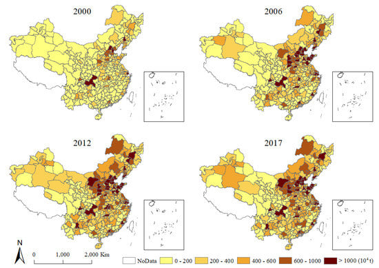
4.1. Spatial Distribution of Carbon Emissions

To analyze the spatiotemporal evolution of carbon emissions over 17 years, we extracted four spatial distribution maps of city-level carbon emissions for the periods 2000 and 2017 (Figure 4). The spatial distribution pattern of carbon emission is found to be similar to previous studies [5,6,11,38]. However, this study additionally detected a pronounced phenomenon that carbon emissions of most cities in China declined during the periods 2012 to 2017.
The high carbon emission regions show an expansive trend and obvious agglomerative characteristics over the past decades. Cities with high carbon emissions mostly agglomerated in the Beijing-Tianjin-Hebei region (BTH) and Yangtze River Delta (YRD). Conversely, cities with low carbon emissions mostly concentrated in the western and central regions. Specifically, there were only three municipalities (Beijing, Shanghai, and Chongqing) whose carbon emissions exceeded 10 million tons in 2000. The number increased to 20 cities in 2006, 30 cities in 2012, but decreased to 21 cities in 2017, indicating that numerous policies on carbon reduction issued by the Chinese government have gained positive response in recent years.
The growth rate analysis of city-level carbon emissions can intuitively present the spatiotemporal trend of carbon emissions. However, earlier studies [5,10,58] focused on contemporaneous comparisons of growth rates of carbon emissions in different cities, ignoring the temporal variations of growth rates of carbon emissions. Thus, we plotted the annual growth type of carbon emissions at each stage (Figure 5). To make the figure clear, we classified the growth rate of city-level carbon emissions into five types: high-negative-growth (−∞, −10%), relatively-high-negative-growth (−10%, 0%), no-obvious-growth (0%, 10%), relatively-high-growth (10%, 20%), high-growth (20%, +∞). From 2000 to 2006, most cities in China were in the phase of rapid growth in carbon emissions during 2006–2012. Cities belonged to relatively-high-growth and high-growth types concentrated in western and central China, where the economic level is relatively low. It is worth noting that few cities have seen significant increases in carbon emissions and almost half of the cites of China have entered the phase of carbon reduction from 2012 on. Compared to the overall country (Figure S2, Supplementary Materials) and provincial level (Figure 3), we see that there is an overall decline in carbon emissions rather than just being evening away from the largest cities. Such a decline in carbon emissions clearly shows that new policy is working effectively, which is followed by one and all in China. However, a very slow balancing between the spatial pattern of high-emission versus low-emission regions in China can be presumed.

4.2. Regional Disparity of Carbon Emissions

Carbon inequality at city-level, indicated by CV (Figure 6), suggests a decreasing trend during the study period, from 1.38 in 2000 to 1.06 in 2017, which is consistent with results of Shi et al. [11] and Wang and Liu [6], and can be interpreted from two opposite aspects: one is from the perspective of high carbon emission areas, and the other is from the perspective of low carbon emission areas. In high carbon emission areas, a series of carbon emissions policies have been implemented, such as improving energy structure and technology, transferring energy-intensive industries to low carbon emissions areas, which facilitate narrowing the gap between high and low carbon emissions regions. On the contrary, low carbon emission areas have scaled up production and emitted more carbon in the course of their economic development. Both development strategies and regional mechanisms have notably reduced carbon inequality [6]. The other reason is that the eastern region has been outsourcing their carbon emissions to western and central regions, which could bear the additional burden of carbon emissions from trading [59,60,61]. For instance, Beijing and Shanghai outsource 50 million tons and 38 million tons of carbon emissions, respectively, for around 70% and 33% of their electricity transmitted from other regions [62].
The Kernel density estimated distributions of carbon emissions over the study period 2012–2017 in China (Figure 7) suggest a significantly skewed shape that demonstrates the existence of carbon inequality at the city level in China. In 2000, the majority of cities show carbon emissions around 600,000 t, and emissions mainly dispersed between 500,000 and 900,000 t. In 2017, carbon emissions mostly concentrated at about 2,000,000 t, and most dispersed between 1,500,000 and 3,000,000 t. The density curve shape (Figure 7) is gradually flattening from 2000 to 2017, indicating that carbon emissions become more evenly distributed between cities, confirming the results measured by CV index. Additionally, the shape of carbon emission density in 2017 is found to be similar to those of 2012, and the CV index shows a slowly decreasing trend from 2010. The dispersion pattern of carbon emissions at the city level in China has stepped into a slow change state.

4.3. Spatial Autocorrelation of Carbon Emissions

Although inequality indicators identify the regional disparity of carbon emissions, the spatial effects are not taken into account. Thus, we introduced Global and Local Moran’s I to evaluate spatial autocorrelation of China’s city-level carbon emissions, and the results were similar to that of earlier studies [6,10]. From Figure 6, we observe that the value of Global Moran’s I has a rising trend, followed by a decline after 2006, while CV shows a sustained downward trend. The CV index reflects only the regional disparity at the quantitative level, but the Global Moran’s I further takes geographic variations into consideration.
The Local Moran’s I can recognize spatial agglomerations and classify them into four types (Figure 8): High-High cluster, Low-Low cluster, Low-High cluster, and High-Low cluster. The two main High-High clusters are mainly located in BTH and YRD. The coverage of High-High cluster located in BTH had been expanding towards west from 2000 to 2017, covering parts around Bohai Gulf area, Shanxi province, Shaanxi province, and Inner Mongolia autonomous region in 2017. The coverage of the High-High cluster concentrated in the YRD remained roughly unchanged during the study period.
The top two city agglomerations in China, BTH, and YRD, followed different development paths of carbon emissions because Beijing is the capital of China and the concentration of national resources, which has been outsourcing its carbon emissions to surrounding cities [61]. Beijing mainly outsourced its carbon emissions to Hebei (22%), Inner Mongolia (7%), and Shanxi (6%) in 2007 [63]. The energy-extensive industry dominated economy in BTH is unrealistic to change in the short term [64], resulting in an expansion of the coverage area of the High-High cluster located here. Thus, energy structure optimization and energy efficiency improvement are the core carbon reduction strategies in the BTH. In contrast, regions in north China account for a larger share of Shanghai’s carbon emissions exports (e.g., Hebei, 9%) than regions around Shanghai (e.g., Jiangsu, 6%) [63]. The pillar industries in the YRD are light industries, such as medium and low-end manufacturing; it is easy to transform them and develop low-carbon “information technology” and high-tech industries. So, industrial structure optimization is the core carbon reduction strategies in the YRD. In addition, most cities belonged the Low-Low cluster distributed in western China, indicating that the carbon emissions of the cities in these backward regions are still in a long-term low emission state. Remarkably, Chengdu, Chongqing, and Wuhan have been the High-Low cluster cities during 2000–2017, for these cities are the central city of the Chengdu-Chongqing and Wuhan Metropolitan Areas, the development of which started late, and the development gap between the central city and surrounding cities is still large. To avoid excessive carbon outsourcing and promote the harmonious development of the whole region, sustainable and coordinated development of cities is the core carbon reduction strategy in these regions. Considering them as a whole, the distribution pattern of carbon emission spatial agglomeration remained unchanged in the periods 2000–2017.

4.4. Uncertainties in the Results

In the present study, city-level carbon emissions for the periods 2000–2017 were calculated through a top-down method by using nighttime light data as a proxy variable. While nighttime light data provide valid information for China, where subnational statistics are limited [44] that could raise some uncertainties:
Firstly, we developed an intercalibration model to integrate the DMSP-OLS data and NPP-VIIRS data to obtain an extended temporal coverage nighttime light data. However, the integration can only be processed with reduced accuracy, resulting in the loss of detailed information detected by VIIRS sensors.
Secondly, point sources like power plants may be ignored by using nighttime light data as a proxy. Nighttime light data is closely related to human activities, while point sources are usually weakly correlated with human activities [65]. For instance, the migration of point sources within the province did not cause drastic changes in DN values but still have an impact on local carbon emissions. This might have resulted in biased estimation of carbon emissions at the city level. However, the limited availability of statistical carbon emissions at the city level makes it unrealistic to calculate the error terms of every city. Earlier studies [5,10] have observed uncertainties as well, and expected that data scarcity may be solved by the National Bureau of Statistics as soon as possible.
Thirdly, the link between nighttime light data and carbon emissions is not strictly linear, which is greatly affected by the way of power generation: reduced emissions with similar to increasing light emissions would be a product of a shift from high (e.g., coal) to low carbon emissions source (e.g., solar). Decreasing carbon emissions accompanied by rising DN values has been observed recently. Although we have shown that our proposed approach is valid so that this phenomenon will not cause many deviations, this non-linear association can provide direct and indirect information about the energy transformation and might become more important in the future. Thus, integration of multiple data and exploration of new methods are required in further studies.
Fourthly, we estimated city-level carbon emissions with city-level nighttime light data. In this step the model coefficients (αp and βp) are kept constant for all cities in a province, just the light data depend on the city. That means, the evaluation indexes of spatiotemporal (CV, Global, and Local Moran’s I) of the estimated emission data actually depend on the covariance structure of the model coefficients (αp and βp) as well as the city light data. However, such problem is inevitable under the data lacking situation.

5. Conclusions

This study introduced nighttime light data as a proxy variable to estimate city-level carbon emissions based on the assumption that nighttime light data has a constant linear relationship with carbon emissions within a specific province. As both DMSP-OLS and NPP-VIIRS time-series nighttime light data have time limits, this study developed a novel method to integrate the data of both sources, extending the temporal coverage during the study period and obtained consistent nighttime light data during the periods 2000–2017. To get the utmost out of the information contained in all samples and improve the estimation accuracy, we built a panel data model linking the integrated nighttime light data and statistical carbon emissions data at the provincial level to recognize their relationships. A top-down method was proposed to estimate city-level carbon emissions by using the coefficient (αp) and intercept (βp) calculated by the panel data model. Such downscaling method of carbon emissions will be useful in monitoring spatiotemporal variations of carbon emissions at other finer scales. These fine scales and timely data provided a basis for assessing the spatiotemporal variations of carbon emissions at the city level.
From the detailed analysis in this study, we found that the cities with low carbon emissions mostly agglomerated in the western and central regions, while cities with high carbon emissions mainly concentrated in the BTH and YRD. In addition, High-High clusters located in the BTH and YRD followed different development paths of carbon emissions during the study period owing to the diverse political status and pillar industries. Indeed, carbon emissions in China have undergone a transformation to decline, while the spatial pattern of carbon emissions in China will not change at a short time. Although, we have found that the effectiveness of our approach may be further enhanced after minimizing some uncertainties in our results. Further improvements need to be made in data scarcity problems, the integration of multiple data, and the exploration of new methods.

Supplementary Materials

The following are available online at https://www.mdpi.com/2072-4292/12/18/2916/s1.

Author Contributions

Conceptualization, Y.S. and S.Z.; methodology, Y.S., S.Z., and U.S.; validation, S.Z. and U.S.; formal analysis, Y.S. and Y.W.; writing—original draft preparation, Y.S.; writing—review and editing, S.Z., R.P.S., and U.S.; visualization, Y.S.; supervision, S.Z. and Y.W.; and funding acquisition, S.Z. All authors have read and agreed to the published version of the manuscript.

Funding

This research was funded by the MOE (Ministry of Education in China) Project of Humanities and Social Sciences (Grant No. 17YJCZH264); the Research Fund for Teaching and Research Development of Liberal Arts Teachers in Zhejiang University; the open fund by Jiangsu Key Laboratory of Atmospheric Environment Monitoring and Pollution Control (KHK1907); and the Opening Project of Shanghai Key Laboratory of Atmospheric Particle Pollution and Prevention (LAP3) (Grant No. FDLAP19003).

Acknowledgments

The authors appreciate NOAA/NCEI for providing annual DMSP-OLS nighttime light data, and CAS for providing annual NPP-VIIRS nighttime light data.

Conflicts of Interest

The authors declare no conflict of interest.

References

  1. Zheng, X.; Lu, Y.; Yuan, J.; Baninla, Y.; Zhang, S.; Stenseth, N.C.; Hessen, D.O.; Tian, H.; Obersteiner, M.; Chen, D. Drivers of change in China’s energy-related CO2 emissions. Proc. Natl. Acad. Sci. USA 2019, 117, 29–36. [Google Scholar] [CrossRef] [PubMed] [Green Version]
  2. Wang, Y.; Luo, X.; Chen, W.; Zhao, M.; Wang, B. Exploring the spatial effect of urbanization on multi-sectoral CO2 emissions in China. Atmos. Pollut. Res. 2019, 10, 1610–1620. [Google Scholar] [CrossRef]
  3. Liu, Y.; Gruber, N.; Brunner, D. Spatiotemporal patterns of the fossil-fuel CO2 signal in central Europe: Results from a high-resolution atmospheric transport model. Atmos. Chem. Phys. Discuss. 2017, 17, 14145–14169. [Google Scholar] [CrossRef] [Green Version]
  4. Clarke-Sather, A.; Qu, J.; Wang, Q.; Zeng, J.; Li, Y. Carbon inequality at the sub-national scale: A case study of provincial-level inequality in CO2 emissions in China 1997–2007. Energy Policy 2011, 39, 5420–5428. [Google Scholar] [CrossRef]
  5. Lv, Q.; Liu, H.; Wang, J.; Liu, H.; Shang, Y. Multiscale analysis on spatiotemporal dynamics of energy consumption CO2 emissions in China: Utilizing the integrated of DMSP-OLS and NPP-VIIRS nighttime light datasets. Sci. Total. Environ. 2020, 703, 134394. [Google Scholar] [CrossRef] [PubMed]
  6. Wang, S.; Liu, X. China’s city-level energy-related CO2 emissions: Spatiotemporal patterns and driving forces. Appl. Energy 2017, 200, 204–214. [Google Scholar] [CrossRef]
  7. Zheng, S.; Shan, J.; Singh, R.P.; Wu, Y.; Pan, J.; Wang, Y.; Lichtfouse, E. High spatio-temporal heterogeneity of carbon footprints in the Zhejiang Province, China, from 2005 to 2015: Implications for climate change policies. Environ. Chem. Lett. 2020, 18, 931–939. [Google Scholar] [CrossRef]
  8. Tobler, W.R. A Computer Movie Simulating Urban Growth in the Detroit Region. Econ. Geogr. 1970, 46, 234. [Google Scholar] [CrossRef]
  9. Liu, X.; Ou, J.; Wang, S.; Li, X.; Yan, Y.; Jiao, L.; Liu, Y. Estimating spatiotemporal variations of city-level energy-related CO2 emissions: An improved disaggregating model based on vegetation adjusted nighttime light data. J. Clean. Prod. 2018, 177, 101–114. [Google Scholar] [CrossRef]
  10. Zhao, J.; Ji, G.; Yue, Y.; Lai, Z.; Chen, Y.; Yang, D.; Yang, X.; Zheng, W. Spatio-temporal dynamics of urban residential CO2 emissions and their driving forces in China using the integrated two nighttime light datasets. Appl. Energy 2019, 235, 612–624. [Google Scholar] [CrossRef]
  11. Shi, K.; Yu, B.; Zhou, Y.; Chen, Y.; Yang, C.; Chen, Z.; Wu, J. Spatiotemporal variations of CO2 emissions and their impact factors in China: A comparative analysis between the provincial and prefectural levels. Appl. Energy 2019, 170–181. [Google Scholar] [CrossRef]
  12. Grunewald, N.; Jakob, M.; Mouratiadou, I. Decomposing inequality in CO2 emissions: The role of primary energy carriers and economic sectors. Ecol. Econ. 2014, 100, 183–194. [Google Scholar] [CrossRef] [Green Version]
  13. Wang, S.; Zhou, C.; Li, G.; Feng, K. CO2, economic growth, and energy consumption in China’s provinces: Investigating the spatiotemporal and econometric characteristics of China’s CO2 emissions. Ecol. Indic. 2016, 69, 184–195. [Google Scholar] [CrossRef]
  14. Wang, S.; Fang, C.; Guan, X.; Pang, B.; Ma, H. Urbanisation, energy consumption, and carbon dioxide emissions in China: A panel data analysis of China’s provinces. Appl. Energy 2014, 136, 738–749. [Google Scholar] [CrossRef]
  15. Cui, Y.; Zhang, W.; Wang, C.; Streets, D.G.; Xu, Y.; Du, M.; Lin, J. Spatiotemporal dynamics of CO2 emissions from central heating supply in the North China Plain over 2012–2016 due to natural gas usage. Appl. Energy 2019, 241, 245–256. [Google Scholar] [CrossRef]
  16. Cui, X.; Lei, Y.; Zhang, F.; Zhang, X.; Wu, F. Mapping spatiotemporal variations of CO2 (carbon dioxide) emissions using nighttime light data in Guangdong Province. Phys. Chem. Earth Parts A B C 2019, 110, 89–98. [Google Scholar] [CrossRef]
  17. Zhao, Z.-Y.; Gao, L.; Zuo, J. How national policies facilitate low carbon city development: A China study. J. Clean. Prod. 2019, 234, 743–754. [Google Scholar] [CrossRef]
  18. Cai, B.; Wang, J.; Yang, S.; Mao, X.; Cao, L. Carbon dioxide emissions from cities in China based on high resolution emission gridded data. Chin. J. Popul. Resour. Environ. 2017, 15, 58–70. [Google Scholar] [CrossRef]
  19. Raupach, M.R.; Rayner, P.J.; Paget, M. Regional variations in spatial structure of nightlights, population density and fossil-fuel CO2 emissions. Energy Policy 2010, 38, 4756–4764. [Google Scholar] [CrossRef]
  20. Yu, B.; Shu, S.; Liu, H.; Song, W.; Wu, J.; Wang, L.; Chen, Z. Object-based spatial cluster analysis of urban landscape pattern using nighttime light satellite images: A case study of China. Int. J. Geogr. Inf. Sci. 2014, 28, 2328–2355. [Google Scholar] [CrossRef]
  21. Cao, X.; Wang, J.; Chen, J.; Shi, F. Spatialization of electricity consumption of China using saturation-corrected DMSP-OLS data. Int. J. Appl. Earth Obs. Geoinf. 2014, 28, 193–200. [Google Scholar] [CrossRef]
  22. Tripathy, B.R.; Sajjad, H.; Elvidge, C.D.; Ting, Y.; Pandey, P.C.; Rani, M.; Kumar, P. Modeling of Electric Demand for Sustainable Energy and Management in India Using Spatio-Temporal DMSP-OLS Night-Time Data. Environ. Manag. 2017, 61, 615–623. [Google Scholar] [CrossRef] [PubMed]
  23. Jasiński, T. Modeling electricity consumption using nighttime light images and artificial neural networks. Energy 2019, 179, 831–842. [Google Scholar] [CrossRef]
  24. Elvidge, C.D.; Baugh, K.E.; Kihn, E.A.; Kroehl, H.W.; Davis, E.R.; Davis, C.W. Relation between satellite observed visible-near infrared emissions, population, economic activity and electric power consumption. Int. J. Remote Sens. 1997, 18, 1373–1379. [Google Scholar] [CrossRef]
  25. Tan, M.; Li, X.; Li, S.; Xin, L.; Wang, X.; Li, Q.; Li, W.; Li, Y.; Xiang, W. Modeling population density based on nighttime light images and land use data in China. Appl. Geogr. 2018, 90, 239–247. [Google Scholar] [CrossRef]
  26. Keola, S.; Andersson, M.; Hall, O. Monitoring Economic Development from Space: Using Nighttime Light and Land Cover Data to Measure Economic Growth. World Dev. 2015, 66, 322–334. [Google Scholar] [CrossRef]
  27. Jing, X.; Shao, X.; Cao, C.; Fu, X.; Yan, L. Comparison between the Suomi-NPP Day-Night Band and DMSP-OLS for Correlating Socio-Economic Variables at the Provincial Level in China. Remote Sens. 2015, 8, 17. [Google Scholar] [CrossRef] [Green Version]
  28. Shi, K.; Yu, B.; Huang, Y.; Hu, Y.; Yin, B.; Chen, Z.; Chen, L.; Wu, J. Evaluating the Ability of NPP-VIIRS Nighttime Light Data to Estimate the Gross Domestic Product and the Electric Power Consumption of China at Multiple Scales: A Comparison with DMSP-OLS Data. Remote Sens. 2014, 6, 1705–1724. [Google Scholar] [CrossRef] [Green Version]
  29. Ma, C.; Niu, Z.; Ma, Y.; Chen, F.; Yang, J.; Liu, J. Assessing the Distribution of Heavy Industrial Heat Sources in India between 2012 and 2018. ISPRS Int. J. Geo-Inf. 2019, 8, 568. [Google Scholar] [CrossRef] [Green Version]
  30. Ma, T.; Zhou, C.; Pei, T.; Haynie, S.; Fan, J. Responses of Suomi-NPP VIIRS-derived nighttime lights to socioeconomic activity in China’s cities. Remote Sens. Lett. 2014, 5, 165–174. [Google Scholar] [CrossRef]
  31. Shi, K.; Yu, B.; Hu, Y.; Huang, C.; Chen, Y.; Huang, Y.; Chen, Z.; Wu, J. Modeling and mapping total freight traffic in China using NPP-VIIRS nighttime light composite data. GIScience Remote Sens. 2015, 52, 274–289. [Google Scholar] [CrossRef]
  32. Xie, Y.; Weng, Q. Spatiotemporally enhancing time-series DMSP/OLS nighttime light imagery for assessing large-scale urban dynamics. ISPRS J. Photogramm. Remote Sens. 2017, 128, 1–15. [Google Scholar] [CrossRef]
  33. Doll, C.; Muller, J.-P.; Elvidge, C.D. Night-time Imagery as a Tool for Global Mapping of Socioeconomic Parameters and Greenhouse Gas Emissions. Ambio 2000, 29, 157–162. [Google Scholar] [CrossRef]
  34. Rayner, P.J.; Raupach, M.R.; Paget, M.; Peylin, P.; Koffi, E. A new global gridded data set of CO2 emissions from fossil fuel combustion: Methodology and evaluation. J. Geophys. Res. Space Phys. 2010, 115, 1–11. [Google Scholar] [CrossRef]
  35. Wu, K.; Wang, X. Aligning Pixel Values of DMSP and VIIRS Nighttime Light Images to Evaluate Urban Dynamics. Remote Sens. 2019, 11, 1463. [Google Scholar] [CrossRef] [Green Version]
  36. Li, X.; Li, D.; Xu, H.; Wu, C. Intercalibration between DMSP/OLS and VIIRS night-time light images to evaluate city light dynamics of Syria’s major human settlement during Syrian Civil War. Int. J. Remote Sens. 2017, 38, 5934–5951. [Google Scholar] [CrossRef]
  37. Zheng, Q.; Weng, Q.; Wang, K. Developing a new cross-sensor calibration model for DMSP-OLS and Suomi-NPP VIIRS night-light imageries. ISPRS J. Photogramm. Remote Sens. 2019, 153, 36–47. [Google Scholar] [CrossRef]
  38. Wang, Z.; Ye, X. Re-examining environmental Kuznets curve for China’s city-level carbon dioxide (CO2) emissions. Spat. Stat. 2017, 21, 377–389. [Google Scholar] [CrossRef]
  39. Version 4 DMSP-OLS Nighttime Lights Time Series. Available online: https://www.ngdc.noaa.gov/eog/dmsp/downloadV4composites.html (accessed on 9 November 2019).
  40. The Chinese Academy of Sciences. Version of the Earth Luminous Data Set (codenamed “Flint”) Provides Annual Data Download Service. Available online: https://www.jianshu.com/p/5fde55a4d267 (accessed on 9 November 2019).
  41. Zhang, X.; Wu, J.; Peng, J.; Cao, Q. The Uncertainty of Nighttime Light Data in Estimating Carbon Dioxide Emissions in China: A Comparison between DMSP-OLS and NPP-VIIRS. Remote Sens. 2017, 9, 797. [Google Scholar] [CrossRef] [Green Version]
  42. Zhu, X.; Ma, M.; Yang, H.; Ge, W. Modeling the Spatiotemporal Dynamics of Gross Domestic Product in China Using Extended Temporal Coverage Nighttime Light Data. Remote Sens. 2017, 9, 626. [Google Scholar] [CrossRef] [Green Version]
  43. Cao, J.; Chen, Y.; Wilson, J.P.; Tan, H.; Yang, J.; Xu, Z. Modeling China’s prefecture-level economy using VIIRS imagery and spatial methods. Remote Sens. 2020, 12, 1–19. [Google Scholar] [CrossRef]
  44. Meng, L.; Graus, W.; Worrell, E.; Huang, B. Estimating CO2 (carbon dioxide) emissions at urban scales by DMSP/OLS (Defense Meteorological Satellite Program’s Operational Linescan System) nighttime light imagery: Methodological challenges and a case study for China. Energy 2014, 71, 468–478. [Google Scholar] [CrossRef]
  45. Shi, K.; Chen, Y.; Yu, B.; Xu, T.; Chen, Z.; Liu, R.; Li, L.; Wu, J. Modeling spatiotemporal CO2 (carbon dioxide) emission dynamics in China from DMSP-OLS nighttime stable light data using panel data analysis. Appl. Energy 2016, 168, 523–533. [Google Scholar] [CrossRef]
  46. Ghosh, T.; Anderson, S.J.; Elvidge, C.D.; Sutton, P.C. Using Nighttime Satellite Imagery as a Proxy Measure of Human Well-Being. Sustainbility 2013, 5, 4988–5019. [Google Scholar] [CrossRef] [Green Version]
  47. Dickey, D.A.; Fuller, W.A. Distribution of the Estimators for Autoregressive Time Series with a Unit Root. J. Am. Stat. Assoc. 1979, 74, 427–431. [Google Scholar] [CrossRef]
  48. Levin, A.; Lin, C.-F.; Chu, C.-S.J. Unit root tests in panel data: Asymptotic and finite-sample properties. J. Econ. 2002, 108, 1–24. [Google Scholar] [CrossRef]
  49. Baltagi, B.H.; Chang, Y.-J. Testing for random individual effects using recursive residuals. Econ. Rev. 1996, 15, 331–338. [Google Scholar] [CrossRef]
  50. Mazor, T.; Levin, N.; Possingham, H.P.; Levy, Y.; Rocchini, D.; Richardson, A.J.; Kark, S. Can satellite-based night lights be used for conservation? The case of nesting sea turtles in the Mediterranean. Biol. Conserv. 2013, 159, 63–72. [Google Scholar] [CrossRef] [Green Version]
  51. Zhang, Q.; Yang, J.; Sun, Z.; Wu, F. Analyzing the impact factors of energy-related CO2 emissions in China: What can spatial panel regressions tell us. J. Clean. Prod. 2017, 161, 1085–1093. [Google Scholar] [CrossRef]
  52. Dhakal, S. Urban energy use and carbon emissions from cities in China and policy implications. Energy Policy 2009, 37, 4208–4219. [Google Scholar] [CrossRef]
  53. Shan, Y.; Liu, J.; Liu, Z.; Shao, S.; Guan, D. An emissions-socioeconomic inventory of Chinese cities. Sci. Data 2019, 6, 1–10. [Google Scholar] [CrossRef] [PubMed] [Green Version]
  54. Paez, A.; Wheeler, D. Geographically Weighted Regression. Int. Encycl. Hum. Geogr. 2009, 28, 407–414. [Google Scholar] [CrossRef]
  55. Lanorte, A.; Danese, M.; Lasaponara, R.; Murgante, B. Multiscale mapping of burn area and severity using multisensor satellite data and spatial autocorrelation analysis. Int. J. Appl. Earth Obs. Geo-Inf. 2013, 20, 42–51. [Google Scholar] [CrossRef]
  56. Moran, P.A.P. The Interpretation of Statistical Maps. J. R. Stat. Soc. 1948, 10, 243–251. [Google Scholar] [CrossRef]
  57. Anselin, L. Local Indicators of Spatial Association-LISA. Geogr. Anal. 2010, 27, 93–115. [Google Scholar] [CrossRef]
  58. Yang, X.; Wang, S.; Zhang, W.; Yu, J. Are the temporal variation and spatial variation of ambient SO2 concentrations determined by different factors. J. Clean. Prod. 2017, 167, 824–836. [Google Scholar] [CrossRef]
  59. Feng, K.; Davis, S.; Sun, L.; Li, X.; Guan, D.; Liu, W.; Liu, Z.; Hubacek, K. Outsourcing CO2 within China. Proc. Natl. Acad. Sci. USA 2013, 110, 11654–11659. [Google Scholar] [CrossRef] [Green Version]
  60. Feng, T.; Du, H.; Zhang, Z.; Mi, Z.; Guan, D.; Zuo, J. Carbon transfer within China: Insights from production fragmentation. Energy Econ. 2020, 86, 104647. [Google Scholar] [CrossRef]
  61. Wang, Z.; Li, Y.; Cai, H.; Wang, B. Comparative analysis of regional carbon emissions accounting methods in China: Production-based versus consumption-based principles. J. Clean. Prod. 2018, 194, 12–22. [Google Scholar] [CrossRef]
  62. Liu, Z.; Guan, D.; Crawford-Brown, D.; Zhang, Q.; He, K.; Liu, J. A low-carbon road map for China. Nature 2013, 500, 143–145. [Google Scholar] [CrossRef]
  63. Feng, K.; Hubacek, K.; Sun, L.; Liu, Z. Consumption-based CO2 accounting of China’s megacities: The case of Beijing, Tianjin, Shanghai and Chongqing. Ecol. Indic. 2014, 47, 26–31. [Google Scholar] [CrossRef]
  64. Xu, L.; Chen, G.; Wiedmann, T.; Wang, Y.; Geschke, A.; Shi, L. Supply-side carbon accounting and mitigation analysis for Beijing-Tianjin-Hebei urban agglomeration in China. J. Environ. Manag. 2019, 248, 109243. [Google Scholar] [CrossRef] [PubMed]
  65. Oda, T.; Maksyutov, S. A very high-resolution (1 km × 1 km) global fossil fuel CO2 emission inventory derived using a point source database and satellite observations of nighttime lights. Atmos. Chem. Phys. Discuss. 2011, 11, 543–556. [Google Scholar] [CrossRef] [Green Version]
Figure 1. Relationship between the total digital pixel numbers (TDN) of the DMSP-OLS and NPP-VIIRS data in 2012 and 2013. The red triangle frames in the picture represent the cities that deviated greatly from the regression line.
Remotesensing 12 02916 g001
Figure 2. Liner relations between the two NPP-VIIRS data at the city level for (a) 2013 and 2014; (b) 2013 and 2015; (c) 2013 and 2016; and (d) 2013 and 2017.
Remotesensing 12 02916 g002
Figure 3. Bar diagram of statistical carbon emissions at the provincial level for the periods 2000–2017.
Remotesensing 12 02916 g003
Figure 4. Spatial distribution of carbon emissions at the city level for the periods 2000–2017.
Remotesensing 12 02916 g004
Figure 5. Growth types of carbon emissions at the city level for the periods 2000–2017.
Remotesensing 12 02916 g005
Figure 6. CV and Global Moran’s I of carbon emissions at the city level for the periods 2000–2017.
Remotesensing 12 02916 g006
Figure 7. Kernel densities of carbon emissions at the city level for the periods 2000–2017.
Remotesensing 12 02916 g007
Figure 8. Spatial autocorrelation of carbon emissions at the city level for the periods 2000–2017.
Remotesensing 12 02916 g008
Table 1. The differences between raw Defense Meteorological Satellite Program’s Operational Linescan System (DMSP-OLS) and Visible Infrared Imaging Radiometer Suite carried by the Suomi National Polar-Orbiting Partnership (NPP-VIIRS) data.
Data SourceDMSP-OLSNPP-VIIRS
Spatial resolution0.008333° (30 arc-seconds)0.004167° (15 arc-seconds)
Radiometric resolution6-bit14-bit
Overpass time19:3001:30
On-board calibrationNoYes
DN range0–630–255
Temporal sequence2000–2013 annual composites2012–2017 annual composites
Table 2. Accuracy assessment comparison of two intercalibration models in 2012.
CityActual DMSP-OLSEarlier ModelProposed Model
Simulated DMSP-OLSRE (%)Simulated DMSP-OLSRE (%)
Beijing295,151182,634−38.62291,495−1.24
Tianjin263,157197,382−26.15261,843−0.50
Shanghai252,233144,852−42.61247,273−1.97
Chongqing208,011249,34814.98212,4612.14
Suzhou272,465181,829−33.81269,128−1.22
Fuyang54,57277,28736.6155,4291.57
Xiamen51,25031,666−38.5950,521−1.42
Heze91,337122,30131.2691,286−0.06
Shangqiu71,604102,93438.1173,0171.97
Zhoukou65,96494,69734.7768,8414.36
Shenzhen113,70255,092−51.56111,414−2.01
Yaan942513,79540.2296382.26
MARE--16-4.95

