Article

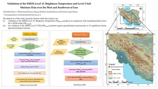
Validation of the SMOS Level 1C Brightness Temperature and Level 2 Soil Moisture Data over the West and Southwest of Iran

by
Mozhdeh Jamei
1,2,*,
Mohammad Mousavi Baygi
1,
Ebrahim Asadi Oskouei
3 and
Ernesto Lopez-Baeza
4
1
Water Science and Engineering Department, Ferdowsi University of Mashhad, Mashhad 9177948974, Iran
2
Khuzestan Water and Power Authority, Ahvaz 61335137, Iran
3
Atmospheric Science and Meteorological Research Center, Tehran 14965114, Iran
4
Climatology from Satellites Group, Earth Physics & Thermodynamics Department, Faculty of Physics, University of Valencia, 46100 Valencia, Spain
*
Author to whom correspondence should be addressed.
Remote Sens. 2020, 12(17), 2819; https://doi.org/10.3390/rs12172819
Submission received: 28 July 2020 / Revised: 28 August 2020 / Accepted: 28 August 2020 / Published: 31 August 2020
(This article belongs to the Special Issue Earth Observation in Support of Sustainable Soils Development)

Abstract

:
The European Space Agency (ESA) Soil Moisture and Ocean Salinity (SMOS) mission with the MIRAS (Microwave Imaging Radiometer using Aperture Synthesis) L-band radiometer provides global soil moisture (SM) data. SM data and products from remote sensing are relatively new, but they are providing significant observations for weather forecasting, water resources management, agriculture, land surface, and climate models assessment, etc. However, the accuracy of satellite measurements is still subject to error from the retrieval algorithms and vegetation cover. Therefore, the validation of satellite measurements is crucial to understand the quality of retrieval products. The objectives of this study, precisely framed within this mission, are (i) validation of the SMOS Level 1C Brightness Temperature (TBSMOS) products in comparison with simulated products from the L-MEB model (TBL-MEB) and (ii) validation of the SMOS Level 2 SM (SMSMOS) products against ground-based measurements at 10 significant Iranian agrometeorological stations. The validations were performed for the period of January 2012 to May 2015 over the Southwest and West of Iran. The results of the validation analysis showed an RMSE ranging between 9 to 13 K and a strong correlation (R = 0.61–0.84) between TBSMOS and TBL-MEB at all stations. The bias values (0.1 to 7.5 K) showed a slight overestimation for TBSMOS at most of the stations. The results of SMSMOS validation indicated a high agreement (RMSE = 0.046–0.079 m3 m−3 and R = 0.65–0.84) between the satellite SM and in situ measurements over all the stations. The findings of this research indicated that SMSMOS shows high accuracy and agreement with in situ measurements which validate its potential. Due to the limitation of SM measurements in Iran, the SMOS products can be used in different scientific and practical applications at different Iranian study areas.

Graphical Abstract

1. Introduction

Surface soil moisture is one of the most significant quantities in the hydrological cycle [1]. It plays a key role in scientific and practical applications such as hydrological modeling [2], numerical weather forecasting [3], flood forecasting [4], drought monitoring [5], water resources management [6], land surface, and climate models assessment, etc. [7] at the local and regional scales. Surface soil moisture is highly variable in space and time [8] due to the spatial heterogeneity of soil properties, topography, rainfall, evapotranspiration [9], and vegetation characteristics. However, direct measurements of ground-based soil moisture are only available at point scale, and measuring this parameter at large scales is significantly costly, time-consuming and, consequently, sparse in most regions. Therefore, these measurements are not practicable for long periods and over wide areas [10].
In recent years, this issue has been overcome using microwave satellite sensors, both active and passive, onboard operational satellites, for measuring soil moisture in different environmental conditions under various vegetation covers [11,12]. L-band (1–2 GHz) microwave radiometry is the most suitable approach to retrieve surface soil moisture [1,13] because it is very sensitive to soil moisture sensing. L-band has a lower atmospheric attenuation and an increased transmissivity in vegetation than higher microwave frequencies (C and X-band) [13,14,15]. Another important advantage of soil moisture retrievals at L-band is that the microwave emission originates from deeper in the soil (~5 cm). In contrast, C-band and X-band emission originates from the top 1 cm or less of the soil [13]. The Advanced Microwave Scanning Radiometer 2 (AMSR2) onboard the Global Change Observation Mission (GCOM)-W1 satellite was launched in May 2012 by the Japan Aerospace Exploration Agency (JAXA) to provide soil moisture at C-band and X-band with grid resolutions of 10 km and 25 km [16,17]. The Advanced Scatterometer (ASCAT) is a C-band (5.255 GHz) active microwave remote sensing instrument onboard the Meteorological Operational (METOP) satellite series to provide global soil moisture data sets with a spatial resolution of 25 or 50 km [18]. Synthetic aperture radar (SAR) provides medium to high resolution mapping of soil moisture in all weather conditions. Sentinel-1 mission provides SAR data at C-band that can be used to retrieve and map temporal changes of soil moisture underneath vegetation cover [12,19,20].
The European Space Agency (ESA) and the National Aeronautics and Space Administration (NASA) have developed respective L-band spaceborne missions to monitor global surface soil moisture over land surfaces that are now operational. NASA launched the Soil Moisture Active Passive (SMAP) satellite in January 2015 carrying an L-band radar (1.26 GHz) and a passive radiometer (1.41 GHz) to provide global monitoring of soil moisture and freeze/thaw [13]. However, the radar instrument stopped working on 7 July 2015 and the SMAP mission continues with its radiometer instrument [21]. Sentinel-1A/Sentinel-1B SAR data was found most suitable for combining with the SMAP radiometer data thanks to its nearly similar orbit configuration, thus allowing overlapping of their swaths with a minimal time difference, a key feature/requirement for the SMAP active-passive algorithm, and being able to obtaining disaggregated brightness temperature, and thus soil moisture at a much finer spatial resolution of 3 km and 1 km at global extent [22]. Previously, in November 2009, ESA had launched the Soil Moisture and Ocean Salinity (SMOS) satellite carrying the first L-band (1.4 GHz) radiometer to provide global soil moisture data over land surfaces and ocean salinity over the oceans [15]. A new innovation of SMOS is the Microwave Imaging Radiometer by Aperture Synthesis (MIRAS) sensor—that is, an L-band 2-D passive microwave interferometry radiometer to provide multi-angular and full polarization brightness temperature measurements with an average ground resolution of 43 km over the field of view (35 km at center of field of view) [23]. The SMOS Level 2 soil moisture algorithm was developed to retrieve soil moisture values (Level 2 SM products) from multi-angular brightness temperature (Level 1C products) with an accuracy of 0.04 m3 m−3 every three days [15,23]. Thus, the validation of SMOS products is very important to determine the accuracy and the quality of retrievals before being used for different applications. Several recent studies have validated SMOS products in comparison to ground-based in situ observations at a global scale [24,25,26,27,28,29] and over local and regional scales such as Canada [30,31], the United States [32,33,34,35,36,37], Europe [37,38,39,40,41,42,43,44], Africa [42,45], and Australia [17,46], and some research has been carried out in Asia such as over the Tibetan Plateau [47,48], Pakistan [49], and China [50,51] that represents the accuracy and the quality of SMOS products. However, very few calibration and validation activities have been done for SMOS products in Iran.
Due to the limited water resources in Iran, there is always a problem of agricultural water supply in most regions. Therefore, availability of regional soil moisture data is essential for the purpose of water resources management, hydrological modeling, and monitoring of droughts. However, in situ soil moisture measurements are currently and operationally taken at only a few agrometeorological stations over Iran, and only for short and discontinuous periods. Due to the scarcity of ground-based soil moisture measurements and scattered agrometeorological stations, the SMOS soil moisture products can be used for different applications. Therefore, the objectives of this research are:
(i)
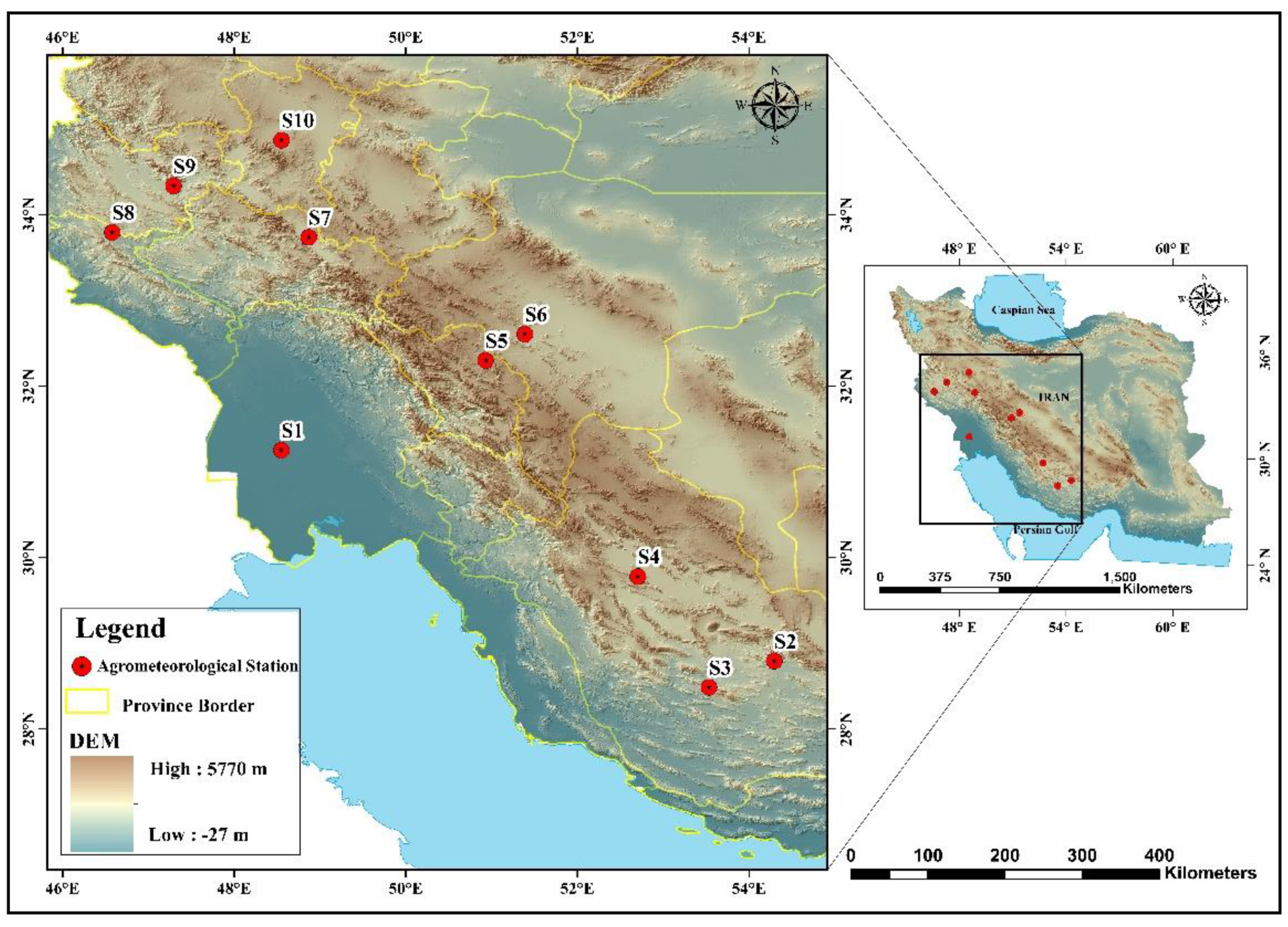
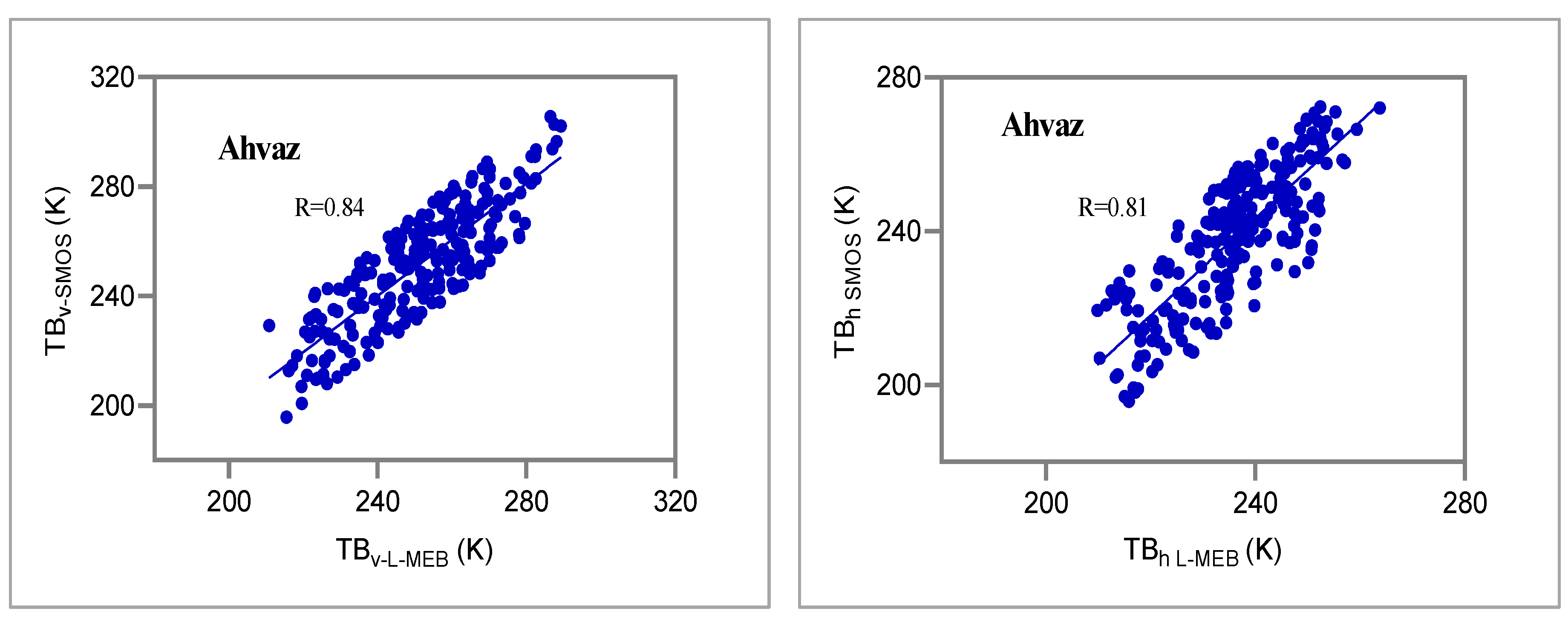
Validation of the SMOS Level 1C Brightness Temperature data products in comparison with the simulated brightness temperature data using of a radiative transfer model (L-MEB model) [52].
(ii)
Validation of the SMOS Level 2 Soil Moisture data products through a comparison with ground-based in situ soil moisture measurements at agrometeorological stations.
These validations were carried out for the period from January 2012 to May 2015 over the Southwest and West of Iran.

2. Materials and Methods
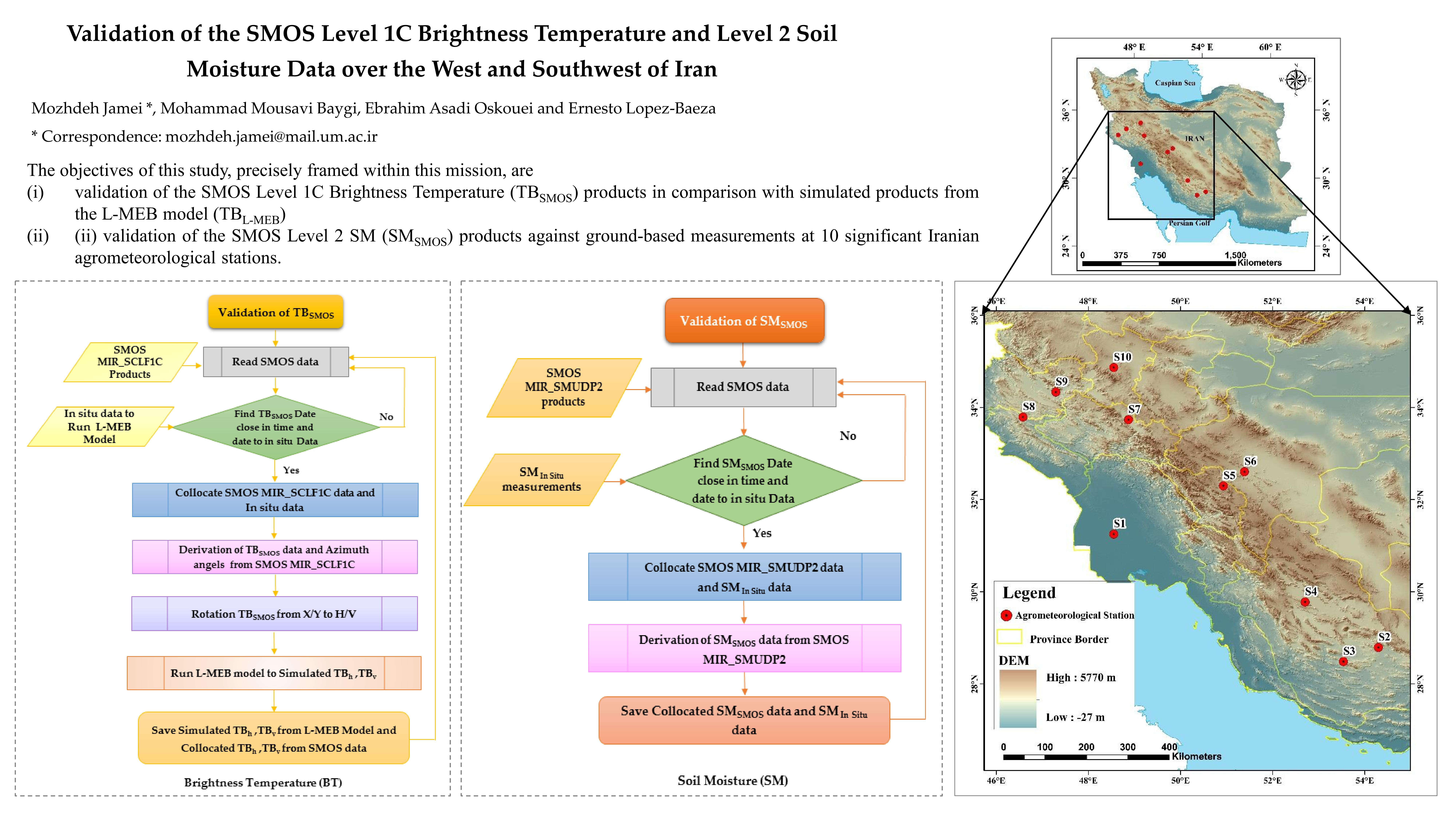
2.1. Study Area

The study area is located in the West and Southwest of Iran within latitude from 28°20′ to 35°15′ N, and longitude from 46°20′ to 54°30′ E. The West and Southwest of Iran is one of the most important agricultural areas of the country, through which Iran’s longest river, the Karun River, flows and in which the largest storage dams and numerous modern irrigation networks are located [53].
The study area can be basically divided into two regions: plane lands and mountainous regions. This region includes 10 agrometeorological stations from the Islamic Republic of Iran Meteorological Organization (IRIMO) which monitors soil moisture data and other climate parameters. In the whole study area, the elevation ranges from about sea level (27 m) to the highest point at about 5770 m. The mean elevation of the selected stations is 1314 m above sea level (m.a.s.l.). In most climate classifications, Iran is generally considered as a semidry or even as a dry country. So, although different stations are located in different climatic areas, the general climate could be considered as semiarid. The geographic coordinates and location of these stations are shown in Figure 1 and Table 1, respectively.

2.2. Ground-Based In Situ Measurements

The International Soil Moisture Network (ISMN) is a centralized data hosting facility that collects and harmonizes in situ soil moisture measurements from various operational networks around the world. The ISMN is an important data base to validate and develop satellite-based soil moisture retrievals [54]. Unfortunately, a significant problem is the limited in situ soil moisture measurements and the absence of ISMN stations in Iran. In this research, to validate the SMOS brightness temperatures and soil moisture observations against ground-based observations, 10 IRIMO agrometeorological stations were used that included measurements of the following parameters: effective soil and vegetation temperatures (air temperature or canopy temperature measured at 5 cm above soil surface level (°C), soil temperature at depths 5 and 50 cm (°C), soil moisture at depth 5 cm (m3 m−3), soil texture, soil bulk density (g cm−3), etc.
IRIMO is under the direction of the World Meteorological Organization (WMO) and subject to its rules and standards. The implementation of the WMO Integrated Global Observing System (WIGOS) relies on the standardization of meteorological and related observations, aiming at uniformity in the practices and procedures employed worldwide and at better accuracy of the observations. WMO prescribes that certain quality control procedures must be applied to all meteorological data and at all stations. Based on WMO standards, IRIMO has applied the data quality control procedures for all agrometeorological stations. All instrumental errors are reported, and related observations have been omitted from the specific station report. Therefore, we used the ground-based in situ observations after IRIMO’s quality control protocol and procedures.
IRIMO has two types of agrometeorological stations including automatic and traditional stations. Time domain reflectometry (TDR) sensors are used to measure soil moisture (at depths 5, 10, 20, 30, 50, 70, and 100 cm) on a daily scale at the agrometeorological automatic stations with an accuracy of 1% volume. Gravimetric techniques are used to measure soil moisture (at depths 5, 10, 20, 30, 50, 70, and 100 cm) on a weekly basis (two or three times) at the traditional agrometeorological stations with an accuracy of 1 mg in weight; the SM sample unit was then transformed from gravimetric (mg mg−1) to volumetric (m3 m−3). In situ measurements from traditional and automatic stations were used to validate the SMOS product. The difference between in situ observations from traditional and automatic stations depends on the accuracy of the measurement method and of the instruments. The characteristics and land cover of the selected stations are shown in Table 2.

2.3. SMOS Satellite and Products

SMOS is the ESA second Earth Explorer opportunity mission developed as part of ESA’s Living Planet Program and it is the first space mission specifically dedicated to measuring global soil moisture over land surfaces [1,23]. The SMOS radiometer measures the radiation emitted from the earth’s surface at the L-band frequency (1.4 GHz). The emissivity at L-band is related to the moisture content in the first few centimeters of soil (typically 5 cm). The 2-D interferometric radiometer is a Y-shaped instrument with three 4.5 m arms which consist of 69 elementary antennas along the arms to measure brightness temperature (TB) at incidence angles between 0° to 60° and for dual or full polarization. The SMOS satellite has a polar sun-synchronous orbit with ascending overpass time at 06:00 and descending overpass time at 18:00 local solar time at the equator, and a mean altitude of 758 km from the Earth [1,15,23].
SMOS satellite data products are generated in several levels: ESA produces data products Level 0 to Level 2, and data products from Level 3 to Level 4 are generated by CNES (Centre National d’Etudes Spatiales, France) and CDTI (Centro para el Desarrollo Tecnológico Industrial, Spain) [1,23,55]. SMOS Level 1C and Level 2 SM products are organized in the Discrete Global Grid (DGG) system which is the ISEA 4H9 grid (quasi equal-area cells all around the globe) with equally spaced nodes at 14.989 km [23].
The SMOS Level 1C Full Polarization Land Science measurements product (MIR_SCLF1C) is organized in the DGG system and each point contains several TBs at the top of the atmosphere (in the reference frame of the SMOS antenna) and associated geophysical parameters for each grid points [56]. The SMOS Level 2 Soil Moisture User Data Product (MIR_SMUDP2) contains retrieved soil moisture, optical thickness, physical temperature, TB computed at 42.5°, and dielectric constants [57]. In this research, we evaluated the SMOS Level 1C Brightness Temperature (TBSMOS) and Level 2 Soil Moisture (SMSMOS) from SMOS MIR_SCLF1C and SMOS MIR_SMUDP2 products, respectively. The version of products used in this study is V620, in Earth Explorer format, with an oversampled resolution of about 15 km.

2.4. The SMOS Level 2 SM Algorithm

The SMOS Level 2 SM algorithm is an operational algorithm to produce soil moisture maps. This algorithm is based on an iterative approach which minimizes a cost function computed from the root mean square difference between SMOS observed TBs (Level 1C products) data at the antenna level and modeled TBs data by L-MEB radiative transfer model over a range of incidence angles. The soil moisture (Level 2 SM products), vegetation optical thickness and other geophysical variables are iteratively retrieved by using the algorithm for each node of DGG [23,52,58].
Validation of satellite remote sensing products is very important, specifically for the SMOS mission due to the unique features of this satellite [33]. So, in the present study, two algorithms were used for the validation of TB SMOS and SM SMOS from MIR_SCLF1C and MIR_SMUDP2 data products, respectively. In the following, the methodology used in these algorithms is explained in detail.

2.4.1. L-MEB Radiative Transfer Model Formulation

The L-MEB (L-band Microwave Emission of the Biosphere) model is a forward model in the SMOS L2 algorithm which has been specifically developed to simulate L-band microwave emission over land surfaces. The L-MEB is the result of comprehensive studies of modeling approaches of passive microwave emission from different land cover types, which is accurate and simple enough for operational use at global scale; therefore, L-MEB is the main reference model to simulate brightness temperature. The L-MEB model is based on a zero-order radiative transfer equation (τ-ω model) in which the main equation of L-MEB is as follows [59,60]:
  T B ( θ , P ) = e s T s γ + ( 1 ω ) ( 1 γ ) T c +   ( 1 ω ) ( 1 γ ) T c ( 1 e s ) γ
where TB is the total TB that depends on the incidence angle (θ) and polarization (P). TB is obtained from the sum of three terms: (1) the soil emission, (2) the direct canopy emission, and (3) the canopy emission reflected by the soil back through the canopy. In this equation, the subscript ‘s’ refers to soil and ‘c’ indicates the canopy. The variable T is the thermodynamic temperature, e is the emissivity, ω is the single scattering albedo of the canopy and γ represents the canopy transmissivity [60].
A pixel of SMOS with the spatial resolution of 43 km over the field of view contains different surface types and so the TB in the L-MEB model is the sum of various classes of emitters [55,56]. In this research, the cover type of selected stations is mainly low vegetation (grassland) and bare soil (desert); in the following, the details of emission from low vegetation and bare soil are presented.

2.4.2. Bare Soil Radiometric Modeling

The brightness temperature of bare soils (TBGP) is a function of soil emissivity (eGP) and of effective soil temperature (TG) as [57]:
TB GP ( θ ) = e GP ( θ ) . T G
where the subscript ‘P’ represents polarization (vertical or horizontal), ‘G’ represents Ground and ‘θ’ is the incidence angle relative to the nadir. eGP is obtained from soil reflectivity (ΓGP) [57]:
e GP ( θ ) = 1 Γ GP ( θ )
ΓGP can be calculated from the Fresnel coefficients as a function of the incidence angle (θ) and the effective soil dielectric constant for smooth soil surfaces. The effective soil dielectric constant is computed by dielectric mixing models with main input parameters such as soil moisture (m3m−3), effective soil temperature (TG, K) and soil properties. More details about dielectric models are described in [52,57]. TG is generally assumed to be independent of polarization and is computed by the following formulation [23,58]:
  T G = T soil _ depth +   C t   ( T soil surf T soil _ depth )
where Tsoil_depth is the deep soil temperature (50 to 100 cm), Tsoil_surf is the surface soil temperature (0 to 5 cm), and the Ct parameter which depends on the frequency band and soil moisture (Ct = 0.246 at L band).

2.4.3. Low Vegetation Radiometric Modeling

The SMOS mission uses the τ−ω model to account for the effects of vegetation which attenuate soil emission and contribute to the emitted radiation. This model uses vegetation optical depth (τP) and single scattering albedo (ωP) to parameterize vegetation attenuation properties and scattering effects within the canopy layer, respectively [23,25,57]. In the τ−ω model, Wigneron et al. [52] assumed that ωP is equal to zero and the effective soil and vegetation temperatures are equal (TG = Tc = TGC) and they presented a simple model to compute the radiative effects of vegetation at L-band as [57]:
TB P = ( 1 γ p 2   Γ GP )   T GC
where TGC is the effective ground–canopy temperature, ΓGP is soil reflectivity, and γP is the vegetation transmissivity which can be computed from τp and the incidence angle (θ) as [57]:
γ P = exp ( τ p   / cos θ )

2.5. Validation of SMOS Brightness Temperature and Soil Moisture Data

In this study, we developed two algorithms based on the L-MEB model to validate TBSMOS and SMSMOS data. The details are as follows.

2.5.1. Validation of TBSMOS Data

Validation of TBSMOS data from MIR_SCLF1C products in the horizontal (H) and vertical (V) polarizations was done through a comparison with simulated TBs data obtained from the L-MEB model [52]. The flow chart of the TBSMOS data validation procedure is shown in Figure 2 and, in the following, details of modeling TBs and validation steps are described. The TBSMOS data was filtered and data with RFI was removed from the analysis. We used SMOS data quality information from ESA Earth Online webpage https://earth.esa.int/web/guest/-/data-quality-7059. To collocate satellite data with ground-based measurements, collocation between the SMOS MIR_SCLF1C data and implied stations was done in space and time. In this study, the time difference between in situ ground-based data and satellite data was considered less than 2 h, and the distance difference between satellite data and stations was considered less than 10 km. For that, the TBSMOS data was selected being nearest to the geographic location of the corresponding stations.
The L-MEB model simulates TBs for various incidence angles using geophysical variables (such as soil moisture, soil temperature, and canopy temperature), soil texture properties, and the radiative transfer parameters. L-MEB simulates L-band surface TBs at the top of atmosphere (TOA) in the Earth reference frame [61]. In this context, Wigneron et al. [52] have developed various terms of the L-MEB equation (Equation (1)) as an algorithm (L-MEB functions) for practical application of modeling TBs in H and V polarizations at incidence angles 0° to 60°, and being Dobson’s, the dielectric mixing model which was used in this work.
Generally, the signal of the microwave sensors is affected by the incidence angle; the sensitivity to soil moisture decreases as incidence angle increases. In addition, the attenuation of vegetation and the effect of surface roughness are minimized at lower incidence angles. Therefore, lower incidence angles are optimal for sensing soil moisture [56,62]. In this study, based on the principle described above and in order to increase the accuracy of modeling brightness temperature, the L-MEB functions were particularized to simulate TBs only at lowest incidence angles. The ground-based in situ measurements (such as air temperature or canopy temperature measured at 5 cm above soil surface level (K); soil temperature at depths 5 and 50 cm (K); soil moisture at depth 5 cm (m3 m−3); soil properties collected from IRIMO stations; and the lowest incidence angles extracted from MIR_SCLF1C products were used as input values for modeling brightness temperature.
In this study, the main limitations in the current application of L-MEB model were related to the assumptions for the vegetation structural parameters related to vegetation optical depth and to soil roughness. For both sets of parameters, we accepted the default values assumed in the L-MEB model.
As mentioned above, the L-MEB model provides TB simulations at the TOA in the Earth reference frame (H/V polarization) whereas the SMOS MIR_SCLF1C products contain TB observations at the TOA in the antenna polarization reference frame (X/Y polarization). In order to compare the satellite TBs and simulated TBs data sets, TBSMOS data sets were transformed from the antenna reference frame (TBx SMOS, TBy SMOS) to the Earth’s surface reference frame (TBH SMOS, TBV SMOS) by using an algorithm (XY2HV) [63] developed by CESBIO (Centre d’Etudes Spatiales de la BIOsphére) team and geometric and Faraday rotations data from SMOS MIR_SCLF1C products.

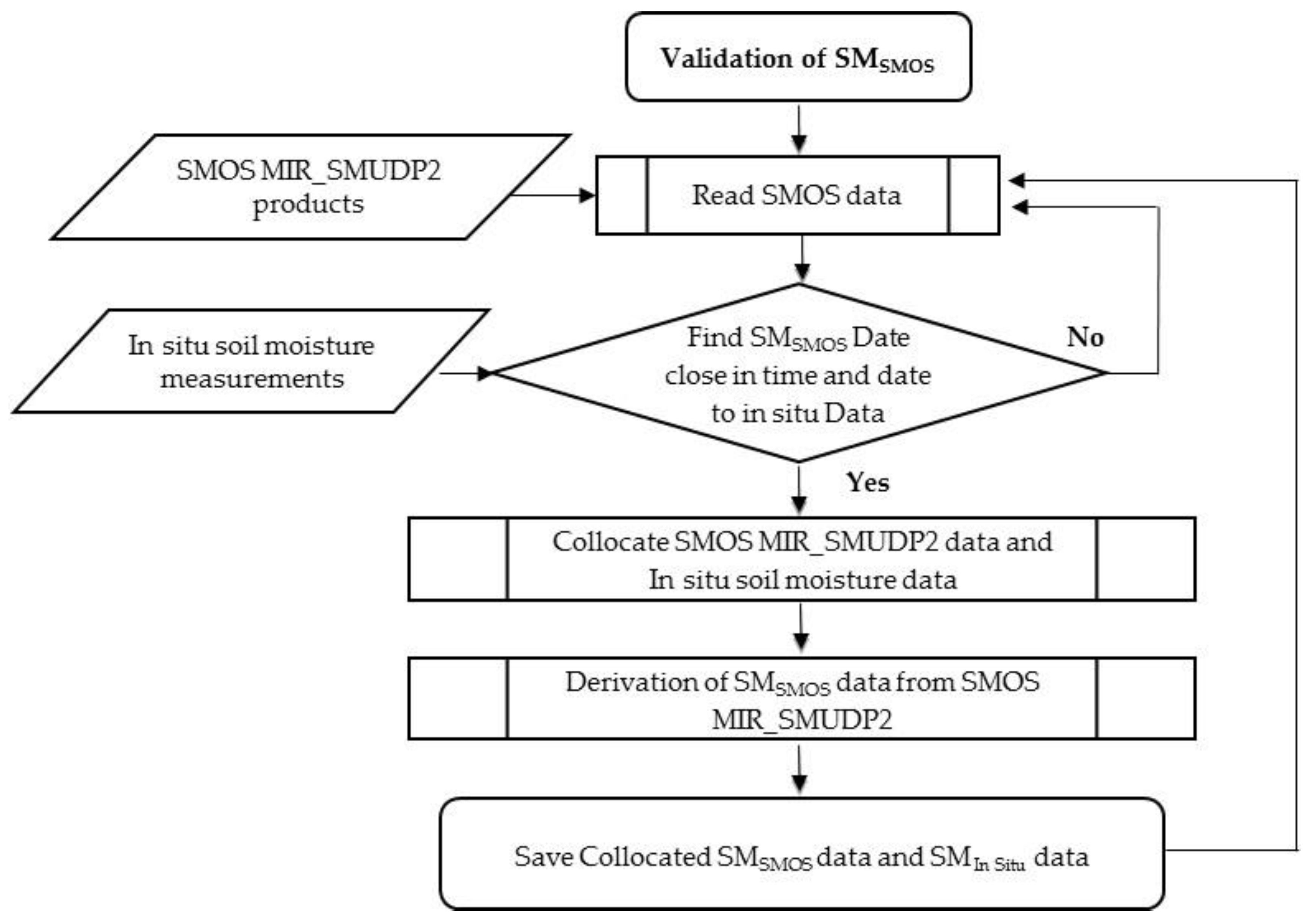
2.5.2. Validation Algorithm for SMSMOS Data

In this the model, the validation of the SMOS soil moisture retrieval data (MIR_SMUDP2 products) was conducted based on comparisons with the ground-based soil moisture measurements. The flow chart of the validation algorithm for SMSMOS data is shown in Figure 3. The SMOS satellite provides global surface soil moisture at a depth of about 0–5 cm [15] and in volumetric units (m3 m−3). Therefore, in order to validate the satellite data, in situ volumetric soil moisture measurements (m3 m−3) collected from all agrometeorological stations were used.
In some cases, during active or following recent rainfall events, the SMOS soil moisture retrieval algorithm tends to overestimate soil moisture as relative to ground measurements, which is related to the contributing depth of the SMOS satellite sensor [30,33]. The temporal variation of soil moisture is between 0.30 and 0.23 m3 m−3 at the first 100 mm soil depth, which soil moisture generally decreased due to evaporation and redistribution at this depth. At a depth of 300 mm, soil moisture varied between 0.50 and 0.47 m3 m−3. This small change in soil moisture could be due to the high clay content of the soil or the fact that there were no plant roots to extract the soil water. At a depth of 600 mm, soil has less soil moisture than at shallow depths since the applied water did not reach this depth. The soil moisture is constant at around 0.21 m3 m−3 a depth of 600 mm [64]. According to the field and laboratory analysis of [64] it should be accepted that SM values should be lower than 0.5 m3 m−3 and, therefore, all SM values above 0.5 m3 m−3 should be excluded. Consequently, in this study, in order to increase the accuracy of the SMOS validation data, if rainfall occurred at the station during a day, the corresponding soil moisture measurements were excluded from the analysis. Examination of SM measurements showed that the SM values were below 0.5 m3 m−3 at all stations after excluding data related to the rainfall days.
In the SMSMOS validation algorithm, the collocation of SMOS MIR_SMUDP2 data with stations was done. Again, the SMOS data was selected based on close geographic proximity to the stations and close temporal proximity to the time measurements at the stations.

2.6. Evaluation Methods

To evaluate TBSMOS and SMSMOS data in comparison with simulated TBs from the L-MEB model (TBL-MEB) and ground-based in situ soil moisture (SMIn situ) data, respectively, four statistical metrics were used. The root-mean-square error (RMSE, (Equation (7)), the mean bias, (Bias, (Equation (8)), the standard deviation, (Std, (Equation (9)), and the Pearson correlation coefficient, (R, (Equation (10)), as follows [14]:
RMSE = 1 N   i = 1 N ( S i M i   ) 2
Bias   = 1 N   i = 1 N   ( S i   M i )
σ S 2 = 1 N i = 1 N   ( S i   S ¯ ) 2 ,   σ M 2 = 1 N i = 1 N   ( M i   M ¯ ) 2
R = 1 ( N 1 ) i = 1 N ( S i   S i   ¯ σ S ) ( M i M i ¯ σ M )
where Si is the SMOS satellite data (TBSMOS/SMSMOS); Mi is the simulated or in situ data (TBL-MEB/SMin situ); N is the total number of observations; σ S is the Std of TBSMOS/SMSMOS data; and σ M is the Std of TBL-MEB/SMin situ.
Taylor diagrams have also been used to represent three different statistical metrics: the correlation coefficient (R), the centered RMSE (cRMSE), and the standard deviation (Std) on two dimensional plots to graphically describe how closely the satellite data (TBSMOS/SMSMOS) matches the simulated TBL-MEB/ observed SMin situ.
In a Taylor diagram, the radial distance from the origin is proportional to the Std, the azimuthal positions indicate the correlation between the satellite data and the observed data, and the cRMSE between the two data sets is the distance to the point on the x-axis marked as “observed”. The satellite data that matches the observations data closely will lie nearest the point “observed” on the x-axis. The R, cRMSE and Std are related by the following Equation [65]:
cRMSE 2 = σ S 2 + σ M 2 2 σ S σ M R

3. Results and Discussion

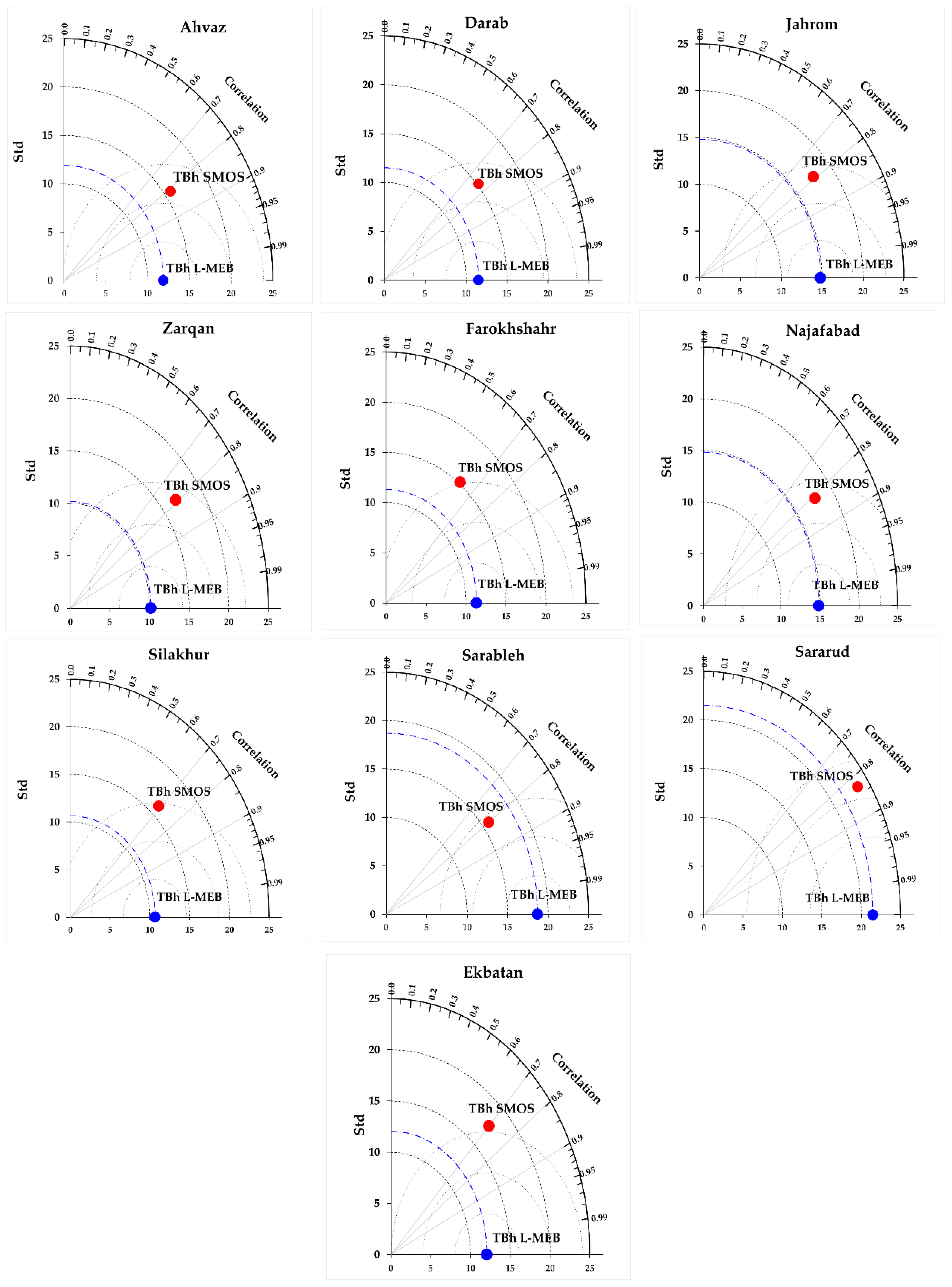
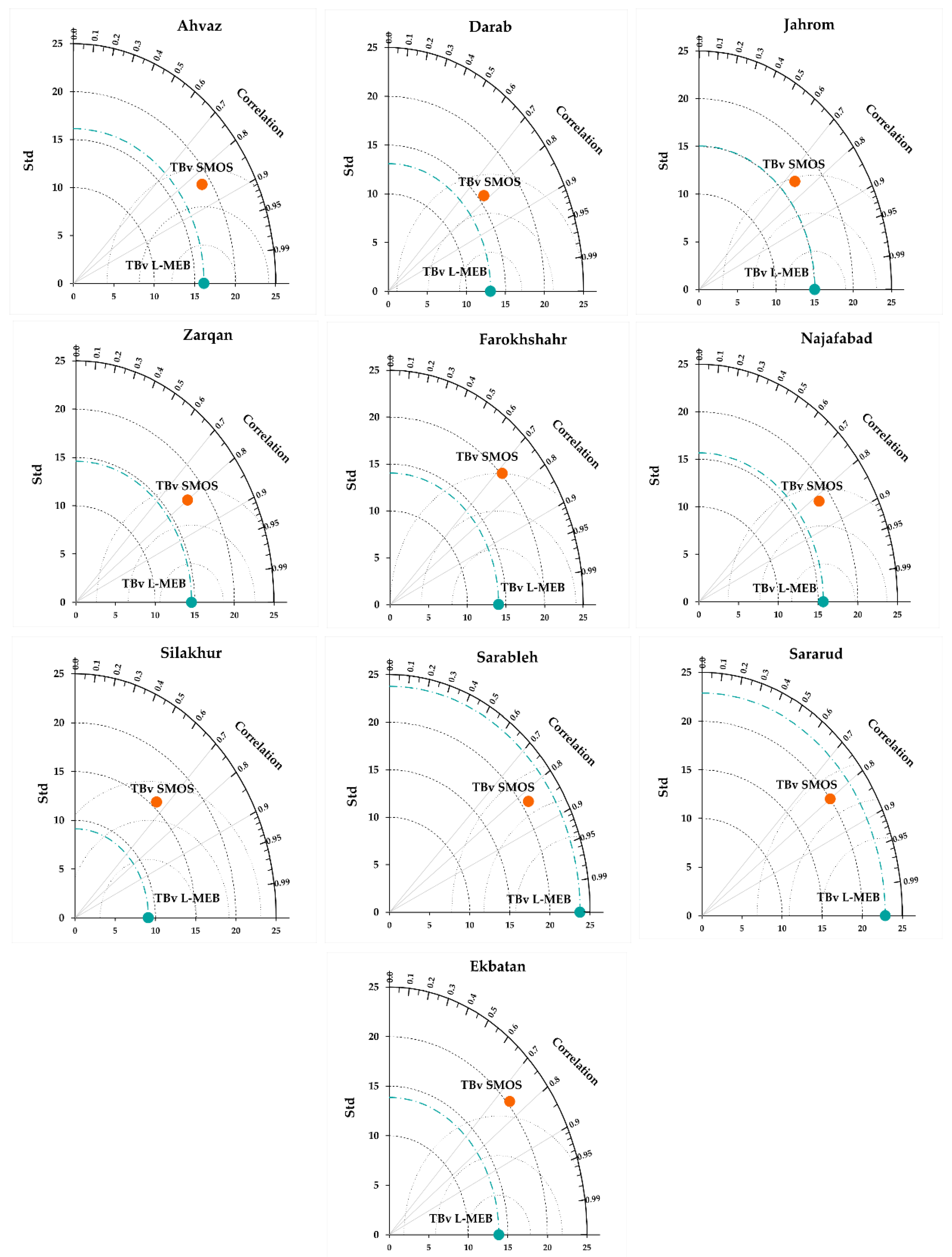
3.1. Validation Results for the SMOS Brightness Temperature

Based on the improved L-MEB model in this study, the simulation of L-band brightness temperature (TBH L-MEB, TBV L-MEB) was done for each station from January 2012 to May 2015. The final TBSMOS validation algorithm outputs were the series of TBH L-MEB and TBV L-MEB data with collocated TBH SMOS and TBV SMOS data from MIR_SCLF1C products at the 10 stations.
The summary of statistical results of the comparison between TBSMOS and TBL-MEB for H and V polarizations are shown in Table 3 and Table 4. The results of Table 3 show that the RMSE values between the TBH SMOS and TBH L-MEB data varied from 9.17 K to 12.88 K. For the Darab, Ahvaz, and Najafabad stations, the TBH SMOS data showed the lowest RMSE values, but for the Farokhshahr and Ekbatan stations, the TBH SMOS data have the highest RMSE values.
The results in Table 4 indicate that the RMSE values of 9.68 K to 12.91 K were found between the TBV SMOS and TBV L-MEB data. The lowest RMSE values of the TBV SMOS data are found over the Ahvaz, Darab, and Najafabad stations, whereas the TBV SMOS data showed the highest RMSE values over the Sarableh, Farokhshahr, and Ekbatan stations.
Results of Table 3 and Table 4 revealed that the cRMSE values of TBH SMOS data were between 9.10 K and 11.94 K, and the cRMSE ranging between 9.50 K and 12.38 K were found for the TBV SMOS data. The positive values of bias in Table 3 indicate a slight overestimation of the TBH SMOS data for most of the stations (Ahvaz, Darab, Jahrom, Zarqan, Silakhur, Sarableh, Sararud, and Ekbatan), whereas the TBH SMOS data with the negative values of bias have a slight underestimation over the Farokhshahr and Najafabad stations. According to the bias values of the TBV SMOS (Table 4), a slight overestimation is found for the Ahvaz, Darab, Jahrom, Zarqan, Farokhshahr, Sarableh, Sararud, and Ekbatan stations. The TBV SMOS data with the negative biases have an underestimation over the Najafabad and Silakhur stations.
Figure 4 shows the result of the comparison between TBSMOS and TBL-MEB values (both H and V polarizations) for Ahvaz station (as an example of station with the highest agreement) in the form of a scatterplot.
The Taylor diagram provides a good way of graphically summarizing the closely matching patterns in terms of R, cRMSE, and their Std [65]. The Taylor diagrams in Figure 5 and Figure 6 illustrate the statistics for the comparison between the SMOS TBs and Simulated TBs data sets for H and V polarizations for all 10 stations. These diagrams reveal the strong correlation between the TBH SMOS and TBH L-MEB (R = 0.61–0.83), and between the TBV SMOS and TBV L-MEB (R = 0.65–0.84) data sets over all stations.
The Taylor diagrams in Figure 5 show that the standard deviations of the TBH SMOS data are close to the TBH L-MEB data at most of the stations (such as Ahvaz, Darab, Jahrom, Farokhshahr, Najafabad, Sarableh, and Sararud) which indicates the same amplitude of variations. Additionally, based on the standard deviation values shown in Figure 6, the TBV SMOS data have very similar spatial variability with the TBV L-MEB data at the Ahvaz, Darab, Jahrom, Zarqan, Najafabad, Sarableh, and Sararud stations.

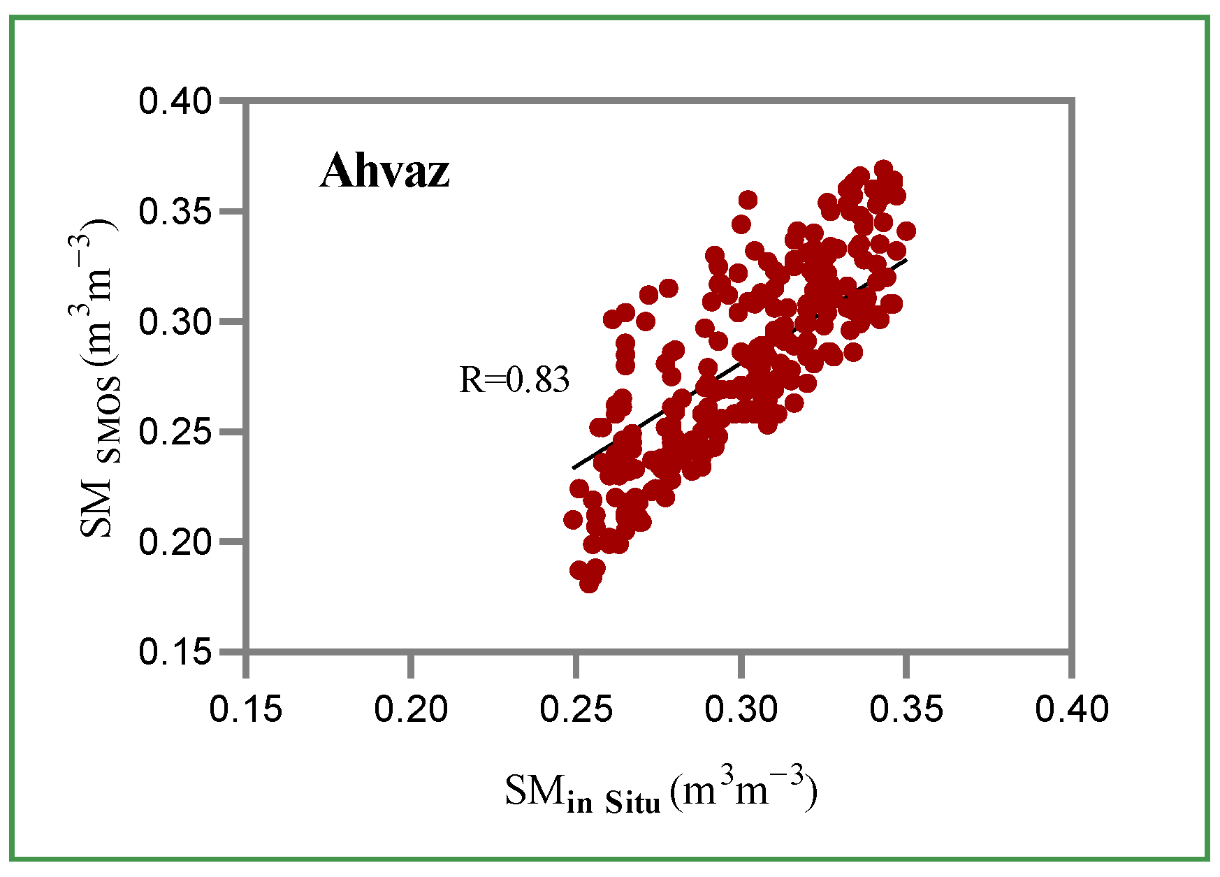
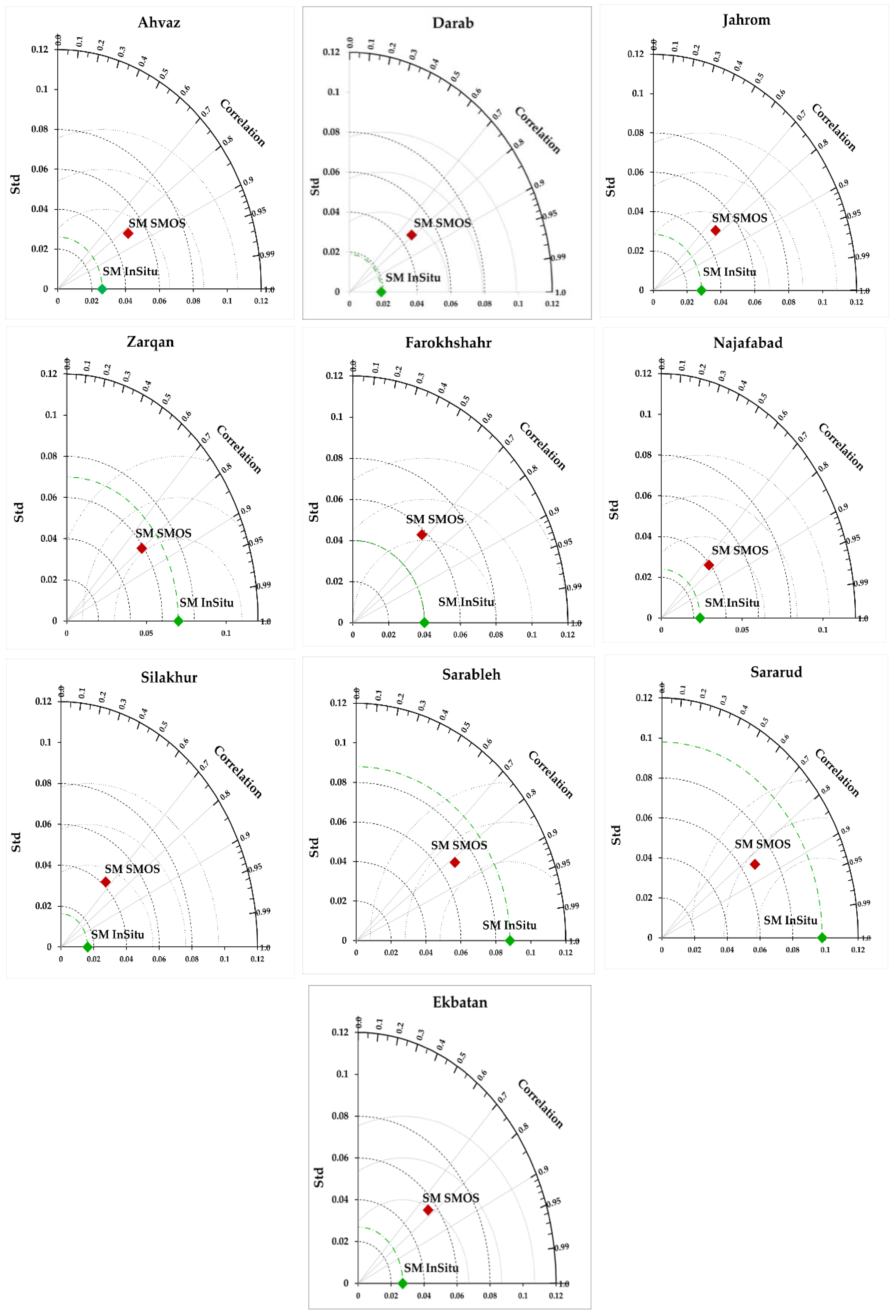
3.2. Validation Results for SMOS Soil Moisture

The validation of SMOS L2 soil moisture retrievals (MIR_SMUDP2 products) was done through a comparison with ground-based in situ measurements collected at the stations using the SMSMOS validation algorithm. This algorithm was run for all stations during the 2012–2015 period. The algorithm outputs were the series of collocated SMOS satellite soil moisture (SMSMOS) data and the ground-based in situ soil moisture measurements (SMin situ) correspondingly matching spatially and temporally. Table 5 presents the results of the statistical metrics. RMSE, cRMSE, bias, correlation coefficient, and standard deviation were used to assess the accuracy of the SMOS soil moisture products over the 10 stations. The comparison between the satellite soil moisture retrieval data and the ground-based measurements reveals that the RMSEs were from 0.046 to 0.079 m3 m−3 over the stations. The SMSMOS data with the lowest RMSE (0.046 m3 m−3) at Ahvaz station is very close to the target accuracy of the SMOS mission, namely RMSE = 0.04 m3 m−3. For the other stations, the SMSMOS data is highly accurate and in agreement with SMin situ data. According to the results of cRMSE values shown in Table 5, the cRMSE ranges of SMSMOS data were between 0.039 to 0.060 m3 m−3. The SMOS products underestimate soil moisture with a slight negative bias in the Ahvaz, Zarqan, Farokhshahr, Ekbatan, Sararud, and Sarableh stations, whereas SMOS products have a slight overestimation in the Darab, Jahrom, Najafabad, and Silakhur stations, as it can be seen in Table 5. Over the Ahvaz station with desert cover (bare soil), SMSMOS data have strong correlation (R = 0.83) with SMin situ data and have the lowest RMSE (0.046 m3 m−3). However, SMSMOS data over the Sararud and Sarableh stations with grassland cover have high correlation (R = 0.84, 0.82, respectively) with SMin situ data, while SMSMOS data have high RMSE over Sarableh (0.079 m3 m−3) and Sararud (0.070 m3 m−3). Figure 7 shows the result of the comparison between the SMSMOS and SMin situ values for Ahvaz station (as an example of station with the highest agreement).
The Taylor diagrams in Figure 8 show the statistical relationship between SMOS soil moisture and ground-based in situ soil moisture measurements at a depth of 5 cm for the selected stations. These diagrams show the strong correlation between the SMSMOS data and SMin situ data (R = 0.65–0.84) at all stations. Based on the standard deviation values shown in the Taylor diagrams (Figure 8), the pattern variations of SMSMOS data were closed to the ground-based measurements (SMin situ) at most of the stations. The Taylor diagram of the Ahvaz station shows that SMOS satellite data with the highest correlation (R = 0.83) and the lowest cRMSE (0.039 m3 m−3) have better agreement with the in situ pattern than other stations. After Ahvaz, the SMSMOS and SMin situ values have high correlation over the Darab, Najafabad, Jahrom, and Zarqan stations (R = 0.79, 0.75, 0.77, and 0.080 m3 m−3, respectively). In these stations, the SMOS data with the low cRMSE (0.046, 0.040, 0.048, and 0.050 m3 m−3, respectively) and high accuracy (RMSE = 0.048, 0.049, 0.050, and 0.059 m3 m−3, respectively) are very close to the SMin situ patterns (Taylor diagrams in Figure 8). The Taylor diagrams for the Ekbatan, Farokhshahr, and Silakhur stations (Figure 8) show the strong correlation of the SMSMOS and SMin situ data (R = 0.77, 0.67, and 0.65, respectively) and the low cRMSE values (0.056, 0.60, and 0.44 m3 m−3). The SMSMOS data have a high correlation with the SMin situ data (R = 0.84 and 0.82) over the Sararud and Sarableh stations but high values of standard deviation and high RMSEs (0.070 and 0.079 m3 m−3) were found for the SMSMOS data in these stations.
Usually, microwave satellite instruments, such as SMOS, provide global SM retrievals at coarse spatial resolutions, so that SM products cannot be directly used for hydrological and agricultural applications at regional and local scales. Surface soil moisture is scale invariant over regimes extending from a satellite footprint to 100 m, such that this assumption can be used for downscaling satellite SM products. The resolution of satellite SM products can be increased through the use of scale invariance properties of soil moisture obtained from hydrologic simulations at hyper-resolutions of less than 100 m [66].

4. Conclusions

For the remote sensing of soil moisture, microwave radiometry at low frequencies (L-band) is the most suitable approach to retrieve surface soil moisture at global scale. The ESA’s SMOS (Soil Moisture and Ocean Salinity) satellite is the first space mission to measure global soil moisture over land surfaces at L-band (1.4 GHz). Validation of SMOS products is crucial to determine the accuracy of retrievals previously used for different applications. The objective of this paper was to assess the accuracy of SMOS products (provided by ESA) over the 10 IRIMO stations in the Southwest and West of Iran for the period 2012 to 2015.
Validation of TBSMOS data from Level 1C products was done through a comparison with the simulated TBs data obtained from the L-MEB model. The radiative transfer L-MEB model was used to simulate TBs with horizontal (H) and vertical (V) polarizations at the lowest SMOS incidence angles over all the stations. The land cover at these stations was either bare soil or low vegetation. Validation of the SMOS retrieved soil moisture data from Level 2 SM product was conducted based on comparisons with in situ ground-based measurements.
The results of the validation between the simulated TB and the TBSMOS data sets showed an RMSE ranging between 9 to 13 K for both H and V polarized channels. The bias ranges between 0.1 to 7.5 K which showed a slight overestimation for the SMOS measurements (both H and V polarizations) compared with the simulated TB at most of the stations. A strong correlation was found between the simulated TB values and the TBSMOS values (R = 0.61 to 0.84) at all stations. The results of SMOS soil moisture validation revealed that the RMSE between the satellite soil moisture retrievals and ground-based in situ measurements ranges from 0.046 to 0.079 m3 m−3 over the stations. These RMSEs are close to the SMOS mission target accuracy of 0.04 m3 m−3. The SMSMOS data was in strong agreement (R = 0.65–0.84) with the in situ soil moisture observations at all stations. According to the results, the SMSMOS products tend to underestimate the soil moisture values with a slight bias values ranging from −0.095 m3m−3 to −0.026 over most of the stations. Overall, the findings of this investigation indicate that the SMSMOS data products are highly accurate and in agreement with in situ data. Due to the scarce in situ SM measurements in Iran, the SMSMOS products can be used to derive soil moisture estimations in the Southwest and West of Iran.
In this study, the important challenges were related to scattered agrometeorological stations, data gaps at the stations, short and discontinuous periods of in situ soil moisture measurements, etc. IRIMO could join ISMN and provide a continuous database with harmonized in situ soil moisture time series from agrometeorological stations over Iran. It will be a very valuable database for the validation of satellite soil moisture products over Iran making this available to all users. The analysis of satellite data could also help to propose IRIMO new agrometeorological stations in unobserved areas where the satellite shows significant SM variations.

Author Contributions

Conceptualization, M.J., M.M.B., and E.L.-B.; data curation, M.J.; formal analysis, M.J.; investigation, M.J.; methodology, M.J.; resources, M.J. and E.A.O.; software, M.J.; supervision, M.M.B. and E.L.-B.; validation, M.J. and E.L.-B.; writing—original draft, M.J.; writing–review and editing, M.J., E.A.O., and E.L.-B. All authors have read and agreed to the published version of the manuscript.

Funding

This research received no external funding.

Acknowledgments

The authors would like to thank the European Space Agency (ESA) for providing the SMOS data and the Islamic Republic of Iran Meteorological Organization (IRIMO) for providing the ground-based data. The authors are also thankful to the University of Maryland for providing opportunities for this research at the Earth System Science Interdisciplinary Center (ESSIC).

Conflicts of Interest

The authors declare no conflict of interest.

References

  1. Kerr, Y.H.; Waldteufel, P.; Wigneron, J.-P.; Martinuzzi, J.-M.; Font, J.; Berger, M. Soil moisture retrieval from space: The Soil Moisture and Ocean Salinity (SMOS) mission. IEEE Trans. Geosci. Remote Sens. 2001, 39, 1729–1735. [Google Scholar] [CrossRef]
  2. Brocca, L.; Moramarco, T.; Melone, F.; Wagner, W.; Hasenauer, S.; Hahn, S. Assimilation of surface-and root-zone ASCAT soil moisture products into rainfall–runoff modeling. IEEE Trans. Geosci. Remote Sens. 2012, 50, 2542–2555. [Google Scholar] [CrossRef]
  3. Dharssi, I.; Bovis, K.; Macpherson, B.; Jones, C. Operational assimilation of ASCAT surface soil wetness at the Met Office. Hydrol. Earth Syst. Sci. 2011, 15, 2729–2746. [Google Scholar] [CrossRef] [Green Version]
  4. Berthet, L.; Andréassian, V.; Perrin, C.; Javelle, P. How crucial is it to account for the antecedent moisture conditions in flood forecasting? Comparison of event-based and continuous approaches on 178 catchments. Hydrol. Earth Syst. Sci. 2009, 13. [Google Scholar] [CrossRef] [Green Version]
  5. Al-Yaari, A.; Wigneron, J.-P.; Kerr, Y.; Rodriguez-Fernandez, N.; O’Neill, P.; Jackson, T.; De Lannoy, G.; Al Bitar, A.; Mialon, A.; Richaume, P. Evaluating soil moisture retrievals from ESA’s SMOS and NASA’s SMAP brightness temperature datasets. Remote Sens. Environ. 2017, 193, 257–273. [Google Scholar] [CrossRef] [PubMed] [Green Version]
  6. Bircher, S.; Skou, N.; Kerr, Y.H.; Member, S. Validation of SMOS L1C and L2 Products and Important Parameters of the Retrieval Algorithm in the Skjern River Catchment, Western Denmark. IEEE Trans. Geosci. Remote Sens. 2013, 51, 2969–2985. [Google Scholar] [CrossRef] [Green Version]
  7. Brocca, L.; Ciabatta, L.; Massari, C.; Camici, S.; Tarpanelli, A.J.W. Soil moisture for hydrological applications: Open questions and new opportunities. Water 2017, 9, 140. [Google Scholar] [CrossRef]
  8. Wagner, W.; Pathe, C.; Doubkova, M.; Sabel, D.; Bartsch, A.; Hasenauer, S.; Blöschl, G.; Scipal, K.; Martínez-Fernández, J.; Löw, A. Temporal stability of soil moisture and radar backscatter observed by the Advanced Synthetic Aperture Radar (ASAR). Sensors 2008, 8, 1174–1197. [Google Scholar] [CrossRef] [Green Version]
  9. Djamai, N.; Magagi, R.; Goita, K.; Merlin, O.; Kerr, Y.; Walker, A. Disaggregation of SMOS soil moisture over the Canadian Prairies. Remote Sens. Environ. 2015, 170, 255–268. [Google Scholar] [CrossRef] [Green Version]
  10. Dall’Amico, J.T. Multiscale Analysis of Soil Moisture Using Satellite and Aircraft Microwave Remote Sensing, in Situ Measurements and Numerical Modelling. Ph.D. Thesis, Ludwig Maximilian University of Munich, Munich, Germany, 2012. [Google Scholar]
  11. Dari, J.; Morbidelli, R.; Saltalippi, C.; Massari, C.; Brocca, L. Spatial-temporal variability of soil moisture: A strategy to optimize monitoring at the catchment scale with varying topography and land use. EGUGA 2018, 20, 7632. [Google Scholar]
  12. Santi, E.; Dabboor, M.; Pettinato, S.; Paloscia, S. Combining machine learning and compact polarimetry for estimating soil moisture from C-band SAR data. Remote Sens. 2019, 11, 2451. [Google Scholar] [CrossRef] [Green Version]
  13. Entekhabi, D.; Njoku, E.G.; Neill, P.E.; Kellogg, K.H.; Crow, W.T.; Edelstein, W.N.; Entin, J.K.; Goodman, S.D.; Jackson, T.J.; Johnson, J. The soil moisture active passive (SMAP) mission. Proc. IEEE 2010, 98, 704–716. [Google Scholar] [CrossRef]
  14. Al-Yaari, A.; Wigneron, J.; Kerr, Y.; De Jeu, R.; Rodriguez-Fernandez, N.; Van Der Schalie, R.; Al Bitar, A.; Mialon, A.; Richaume, P.; Dolman, A. Testing regression equations to derive long-term global soil moisture datasets from passive microwave observations. Remote Sens. Environ. 2016, 180, 453–464. [Google Scholar] [CrossRef]
  15. Kerr, Y.H.; Waldteufel, P.; Wigneron, J.-P.; Delwart, S.; Cabot, F.O.; Boutin, J.; Escorihuela, M.-J.; Font, J.; Reul, N.; Gruhier, C. The SMOS mission: New tool for monitoring key elements ofthe global water cycle. Proc. IEEE 2010, 98, 666–687. [Google Scholar] [CrossRef] [Green Version]
  16. Parinussa, R.M.; Holmes, T.R.; Wanders, N.; Dorigo, W.A.; de Jeu, R.A. A preliminary study toward consistent soil moisture from AMSR2. J. Hydrometeorol. 2015, 16, 932–947. [Google Scholar] [CrossRef]
  17. Yee, M.S.; Walker, J.P.; Rüdiger, C.; Parinussa, R.M.; Koike, T.; Kerr, Y.H. A comparison of SMOS and AMSR2 soil moisture using representative sites of the OzNet monitoring network. Remote Sens. Environ. 2017, 195, 297–312. [Google Scholar] [CrossRef]
  18. Wagner, W.; Hahn, S.; Kidd, R.; Melzer, T.; Bartalis, Z.; Hasenauer, S.; Figa-Saldaña, J.; De Rosnay, P.; Jann, A.; Schneider, S. The ASCAT soil moisture product: A review of its specifications, validation results, and emerging applications. Meteorol. Z. 2013, 22, 5–33. [Google Scholar] [CrossRef] [Green Version]
  19. Bousbih, S.; Zribi, M.; Lili-Chabaane, Z.; Baghdadi, N.; El Hajj, M.; Gao, Q.; Mougenot, B. Potential of Sentinel-1 radar data for the assessment of soil and cereal cover parameters. Sensors 2017, 17, 2617. [Google Scholar] [CrossRef] [Green Version]
  20. Gao, Q.; Zribi, M.; Escorihuela, M.J.; Baghdadi, N.; Segui, P.Q. Irrigation mapping using Sentinel-1 time series at field scale. Remote Sens. 2018, 10, 1495. [Google Scholar] [CrossRef] [Green Version]
  21. O’Neill, P.E.; Chan, S.; Njoku, E.G.; Jackson, T.; Bindlish, R. Soil Moisture Active Passive (SMAP) Algorithm Theoretical Basis Document Level 2 & 3 Soil Moisture (Passive) Data Products; Jet Propulsion Laboratory California Institute of Technology: Pasadena, CA, USA, 2018; pp. 1–82. [Google Scholar]
  22. Das, N.N.; Entekhabi, D.; Dunbar, R.S.; Chaubell, M.J.; Colliander, A.; Yueh, S.; Jagdhuber, T.; Chen, F.; Crow, W.; O’Neill, P.E. The SMAP and copernicus sentinel 1A/B microwave active-passive high resolution surface soil moisture product. Remote Sens. Environ. 2019, 233, 111380. [Google Scholar] [CrossRef]
  23. Kerr, Y.H.; Waldteufel, P.; Richaume, P.; Wigneron, J.P.; Ferrazzoli, P.; Mahmoodi, A.; Al Bitar, A.; Cabot, F.; Gruhier, C.; Juglea, S.E. The SMOS soil moisture retrieval algorithm. IEEE Trans. Geosci. Remote Sens. 2012, 50, 1384–1403. [Google Scholar] [CrossRef]
  24. Al-Yaari, A.; Wigneron, J.-P.; Ducharne, A.; Kerr, Y.; De Rosnay, P.; De Jeu, R.; Govind, A.; Al Bitar, A.; Albergel, C.; Munoz-Sabater, J. Global-scale evaluation of two satellite-based passive microwave soil moisture datasets (SMOS and AMSR-E) with respect to Land Data Assimilation System estimates. Remote Sens. Environ. 2014, 149, 181–195. [Google Scholar] [CrossRef] [Green Version]
  25. Al-Yaari, A.; Wigneron, J.-P.; Ducharne, A.; Kerr, Y.; Wagner, W.; De Lannoy, G.; Reichle, R.; Al Bitar, A.; Dorigo, W.; Richaume, P. Global-scale comparison of passive (SMOS) and active (ASCAT) satellite based microwave soil moisture retrievals with soil moisture simulations (MERRA-Land). Remote Sens. Environ. 2014, 152, 614–626. [Google Scholar] [CrossRef] [Green Version]
  26. Kerr, Y.H.; Al-Yaari, A.; Rodriguez-Fernandez, N.; Parrens, M.; Molero, B.; Leroux, D.; Bircher, S.; Mahmoodi, A.; Mialon, A.; Richaume, P. Overview of SMOS performance in terms of global soil moisture monitoring after six years in operation. Remote Sens. Environ. 2016, 180, 40–63. [Google Scholar] [CrossRef]
  27. Leroux, D.J.; Kerr, Y.H.; Richaume, P.; Fieuzal, R. Spatial distribution and possible sources of SMOS errors at the global scale. Remote Sens. Environ. 2013, 133, 240–250. [Google Scholar] [CrossRef] [Green Version]
  28. Albergel, C.; De Rosnay, P.; Gruhier, C.; Muñoz-Sabater, J.; Hasenauer, S.; Isaksen, L.; Kerr, Y.; Wagner, W. Evaluation of remotely sensed and modelled soil moisture products using global ground-based in situ observations. Remote Sens. Environ. 2012, 118, 215–226. [Google Scholar] [CrossRef]
  29. Al Bitar, A.; Mialon, A.; Kerr, Y.H.; Cabot, F.; Richaume, P.; Jacquette, E.; Quesney, A.; Mahmoodi, A.; Tarot, S.; Parrens, M.; et al. The global SMOS Level 3 daily soil moisture and brightness temperature maps. Earth Syst. Sci. Data 2017, 9, 293–315. [Google Scholar] [CrossRef] [Green Version]
  30. Champagne, C.; Rowlandson, T.; Berg, A.; Burns, T.; L’Heureux, J.; Tetlock, E.; Adams, J.R.; McNairn, H.; Toth, B.; Itenfisu, D. Satellite surface soil moisture from SMOS and Aquarius: Assessment for applications in agricultural landscapes. Int. J. Appl. Earth Obs. Geoinf. 2016, 45, 143–154. [Google Scholar] [CrossRef] [Green Version]
  31. Djamai, N.; Magagi, R.; Goïta, K.; Hosseini, M.; Cosh, M.H.; Berg, A.; Toth, B. Evaluation of SMOS soil moisture products over the CanEx-SM10 area. J. Hydrol. 2015, 520, 254–267. [Google Scholar] [CrossRef]
  32. Al Bitar, A.; Leroux, D.; Kerr, Y.H.; Merlin, O.; Richaume, P.; Sahoo, A.; Wood, E.F. Evaluation of SMOS soil moisture products over continental US using the SCAN/SNOTEL network. IEEE Trans. Geosci. Remote Sens. 2012, 50, 1572–1586. [Google Scholar] [CrossRef] [Green Version]
  33. Jackson, T.J.; Bindlish, R.; Cosh, M.H.; Zhao, T.; Starks, P.J.; Bosch, D.D.; Seyfried, M.; Moran, M.S.; Goodrich, D.C.; Kerr, Y.H. validation of soil moisture and ocean salinity (SMOS) soil moisture over watershed networks in the US. IEEE Trans. Geosci. Remote Sens. 2012, 50, 1530–1543. [Google Scholar] [CrossRef] [Green Version]
  34. Leroux, D.J.; Kerr, Y.H.; Al Bitar, A.; Bindlish, R.; Jackson, T.J.; Berthelot, B.; Portet, G. Comparison between SMOS, VUA, ASCAT, and ECMWF soil moisture products over four watersheds in US. IEEE Trans. Geosci. Remote Sens. 2014, 52, 1562–1571. [Google Scholar] [CrossRef] [Green Version]
  35. Wagner, W.; Brocca, L.; Naeimi, V.; Reichle, R.; Draper, C.; De Jeu, R.; Ryu, D.; Su, C.H.; Western, A.; Calvet, J.C.; et al. Clarifications on the “comparison between SMOS, VUA, ASCAT, and ECMWF Soil Moisture Products over Four Watersheds in U.S.”. IEEE Trans. Geosci. Remote Sens. 2014, 52, 1901–1906. [Google Scholar] [CrossRef]
  36. Walker, V.A.; Hornbuckle, B.K.; Cosh, M.H. A five-year evaluation of SMOS Level 2 soil moisture in the corn belt of the United States. IEEE J. Sel. Top. Appl. Earth Obs. Remote Sens. 2018, 11, 4664–4675. [Google Scholar] [CrossRef]
  37. Cui, C.; Xu, J.; Zeng, J.; Chen, K.-S.; Bai, X.; Lu, H.; Chen, Q.; Zhao, T. Soil moisture mapping from satellites: An intercomparison of SMAP, SMOS, FY3B, AMSR2, and ESA CCI over two dense network regions at different spatial scales. Remote Sens. 2018, 10, 33. [Google Scholar] [CrossRef] [Green Version]
  38. Dall’Amico, J.T.; Schlenz, F.; Loew, A.; Mauser, W. First Results of SMOS Soil Moisture Validation in the Upper Danube Catchment. IEEE Trans. Geosci. Remote Sens. 2012, 50, 1507–1516. [Google Scholar] [CrossRef]
  39. El Hajj, M.; Baghdadi, N.; Zribi, M.; Rodríguez-Fernández, N.; Wigneron, J.P.; Al-Yaari, A.; Al Bitar, A.; Albergel, C.; Calvet, J.-C. Evaluation of SMOS, SMAP, ASCAT and sentinel-1 soil moisture products at sites in Southwestern France. Remote Sens. 2018, 10, 569. [Google Scholar] [CrossRef] [Green Version]
  40. Gonzalez-Zamora, A.; Sanchez, N.; Gumuzzio, A.; Piles, M.; Olmedo, E.; Martínez-Fernández, J. Validation of SMOS L2 and L3 soil moisture products over the Duero basin at different spatial scales. ISPRS Arch. 2015, 40, 1183–1188. [Google Scholar] [CrossRef] [Green Version]
  41. Montzka, C.; Bogena, H.R.; Weihermüller, L.; Jonard, F.; Bouzinac, C.; Kainulainen, J.; Balling, J.E.; Loew, A.; Amico, J.T.; Rouhe, E.; et al. brightness temperature and soil moisture validation at different scales during the SMOS validation campaign in the rur and erft catchments, Germany. IEEE Trans. Geosci. Remote Sens. 2013, 51, 1728–1743. [Google Scholar] [CrossRef]
  42. Pierdicca, N.; Pulvirenti, L.; Fascetti, F.; Crapolicchio, R.; Talone, M. Analysis of two years of ASCAT-and SMOS-derived soil moisture estimates over Europe and North Africa. Eur. J. Remote Sens. 2013, 46, 759–773. [Google Scholar] [CrossRef]
  43. Sánchez, N.; Martínez-fernández, J.; Scaini, A.; Pérez-gutiérrez, C. Validation of the SMOS L2 Soil Moisture Data in the REMEDHUS Network (Spain). IEEE Trans. Geosci. Remote Sens. 2012, 50, 1602–1611. [Google Scholar] [CrossRef]
  44. Wigneron, J.-P.; Schwank, M.; Baeza, E.L.; Kerr, Y.; Novello, N.; Millan, C.; Moisy, C.; Richaume, P.; Mialon, A.; Al Bitar, A. First evaluation of the simultaneous SMOS and ELBARA-II observations in the Mediterranean region. Remote Sens. Environ. 2012, 124, 26–37. [Google Scholar] [CrossRef]
  45. Louvet, S.; Pellarin, T.; al Bitar, A.; Cappelaere, B.; Galle, S.; Grippa, M.; Gruhier, C.; Kerr, Y.; Lebel, T.; Mialon, A.; et al. SMOS soil moisture product evaluation over West-Africa from local to regional scale. Remote Sens. Environ. 2015, 156, 383–394. [Google Scholar] [CrossRef]
  46. Su, C.-H.; Ryu, D.; Young, R.I.; Western, A.W.; Wagner, W. Inter-comparison of microwave satellite soil moisture retrievals over the Murrumbidgee Basin, Southeast Australia. Remote Sens. Environ. 2013, 134, 1–11. [Google Scholar] [CrossRef]
  47. Chen, Y.; Yang, K.; Qin, J.; Cui, Q.; Lu, H.; La, Z.; Han, M.; Tang, W. Evaluation of SMAP, SMOS, and AMSR2 soil moisture retrievals against observations from two networks on the Tibetan Plateau. J. Geophys. Res. Atmos. 2017, 122, 5780–5792. [Google Scholar] [CrossRef]
  48. Zhao, L.; Yang, K.; Qin, J.; Chen, Y.; Tang, W.; Lu, H.; Yang, Z.-L. The scale-dependence of SMOS soil moisture accuracy and its improvement through land data assimilation in the central Tibetan Plateau. Remote Sens. Environ. 2014, 152, 345–355. [Google Scholar] [CrossRef]
  49. Anam, R.; Chishtie, F.; Ghuffar, S.; Qazi, W.; Shahid, I. Inter-comparison of SMOS and AMSR-E soil moisture products during flood years (2010–2011) over Pakistan. Eur. J. Remote Sens. 2017, 50, 442–451. [Google Scholar] [CrossRef] [Green Version]
  50. Cui, H.; Jiang, L.; Du, J.; Zhao, S.; Wang, G.; Lu, Z.; Wang, J. Evaluation and analysis of AMSR-2, SMOS, and SMAP soil moisture products in the Genhe area of China. J. Geophys. Res. Atmos. 2017, 122, 8650–8666. [Google Scholar] [CrossRef]
  51. Zhang, L.; He, C.; Zhang, M.; Zhu, Y. Evaluation of the SMOS and SMAP soil moisture products under different vegetation types against two sparse in situ networks over arid mountainous watersheds, Northwest China. Sci. Chin. Earth Sci. 2019, 62, 703–718. [Google Scholar] [CrossRef]
  52. Wigneron, J.-P.; Kerr, Y.; Waldteufel, P.; Saleh, K.; Escorihuela, M.-J.; Richaume, P.; Ferrazzoli, P.; De Rosnay, P.; Gurney, R.; Calvet, J.-C. L-band Microwave Emission of the Biosphere (L-MEB) Model: Description and calibration against experimental data sets over crop fields. Remote Sens. Environ. 2007, 107, 639–655. [Google Scholar] [CrossRef]
  53. Jamei, M. Validation of SMOS Satellite Data to Estimate Soil Moisture (A Case Study: West and South-West of Iran). Ph.D. Thesis, Ferdowsi University of Mashhad, Mashhad, Iran, 2018. [Google Scholar]
  54. Dorigo, W.; Wagner, W.; Hohensinn, R.; Hahn, S.; Paulik, C.; Xaver, A.; Gruber, A.; Drusch, M.; Mecklenburg, S.; Oevelen, P.v. The international soil moisture network: A data hosting facility for global in situ soil moisture measurements. Hydrol. Earth Syst. Sci. 2011, 15, 1675–1698. [Google Scholar] [CrossRef] [Green Version]
  55. Kerr, Y.; Waldteufel, P.; Richaume, P.; Wigneron, J.; Ferrazzoli, P.; Gurney, R. SMOS Level 2 Processor for Soil Moisture—Algorithm Theoretical Based Document (ATBD); Technical Report SO-TN-ESL-SM-GS-0001; CESBIO: Toulouse, France, 2015. [Google Scholar]
  56. Al-Yaari, A.M. Global-Scale Evaluation of a Hydrological Variable Measured from Space: SMOS Satellite Remote Sensing Soil Moisture Products. Ph.D. Thesis, Université Pierre et Marie Curie-Paris VI, Paris, France, 2014. [Google Scholar]
  57. Wigneron, J.-P.; Jackson, T.; O’Neill, P.; De Lannoy, G.; de Rosnay, P.; Walker, J.; Ferrazzoli, P.; Mironov, V.; Bircher, S.; Grant, J. Modelling the passive microwave signature from land surfaces: A review of recent results and application to the L-band SMOS & SMAP soil moisture retrieval algorithms. Remote Sens. Environ. 2017, 192, 238–262. [Google Scholar]
  58. Wigneron, J.-P.; Chanzy, A.; De Rosnay, P.; Rudiger, C.; Calvet, J.-C. Estimating the effective soil temperature at L-band as a function of soil properties. IEEE Trans. Geosci. Remote Sens. 2008, 46, 797–807. [Google Scholar] [CrossRef]
  59. Wigneron, J.-P.; Chanzy, A.; Kerr, Y.H.; Lawrence, H.; Shi, J.; Escorihuela, M.J.; Mironov, V.; Mialon, A.; Demontoux, F.; De Rosnay, P. Evaluating an improved parameterization of the soil emission in L-MEB. IEEE Trans. Geosci. Remote Sens. 2011, 49, 1177–1189. [Google Scholar] [CrossRef]
  60. Grant, J.P.; Wigneron, J.-P.; Van de Griend, A.A.; Guglielmetti, M.; Saleh, K.; Schwank, M. Calibration of L-MEB for soil moisture retrieval over forests. In Proceedings of the IEEE International Geoscience and Remote Sensing Symposium IGARSS 2007, Barcelona, Spain, 23–28 July 2017; pp. 2248–2251. [Google Scholar]
  61. Montzka, C.; Grant, J.P.; Moradkhani, H.; Franssen, H.-J.H.; Weihermüller, L.; Drusch, M.; Vereecken, H. Estimation of radiative transfer parameters from L-band passive microwave brightness temperatures using advanced data assimilation. Vadose Zone J. 2013, 12, 1–17. [Google Scholar] [CrossRef] [Green Version]
  62. Ulaby, F.T.; Moore, R.K.; Fung, A.K. Microwave Remote Sensing Active and Passive-Volume III: From Theory to Applications; Artech House: Norwood, MA, USA, 1986. [Google Scholar]
  63. Yumpu. Available online: https://www.yumpu.com/en/document/read/36615690/rwapi-and-xy2hv-transformation-cesbio (accessed on 20 July 2020).
  64. Gebregiorgis, M.F.; Savage, M.J. Field, laboratory and estimated soil-water content limits. Water SA 2006, 32, 155–162. [Google Scholar] [CrossRef] [Green Version]
  65. Taylor, K.E. Summarizing multiple aspects of model performance in a single diagram. J. Geophys. Res. Atmos. 2001, 106, 7183–7192. [Google Scholar] [CrossRef]
  66. Mascaro, G.; Ko, A.; Vivoni, E.R. Closing the loop of satellite soil moisture estimation via scale invariance of hydrologic simulations. Sci. Rep. 2019, 9, 1–8. [Google Scholar] [CrossRef] [Green Version]
Figure 1. Study area: geographical location of agrometeorological stations.
Remotesensing 12 02819 g001
Figure 2. Flow chart of TBSMOS data validation algorithm.
Remotesensing 12 02819 g002
Figure 3. Flow chart of SMSMOS data validation algorithm.
Remotesensing 12 02819 g003
Figure 4. The scatterplots of the TBSMOS against the TBL-MEB for Ahvaz station. The left plot for H polarization and right plot for V polarization.
Remotesensing 12 02819 g004
Figure 5. Taylor diagrams illustrating the statistics of the comparisons between TBH SMOS and TBH L-MEB data.
Remotesensing 12 02819 g005
Figure 6. Taylor diagrams illustrating the statistics of the comparisons between TBV SMOS and TBV L-MEB data.
Remotesensing 12 02819 g006
Figure 7. The scatterplots of SM SMOS against SM in situ for Ahvaz station.
Remotesensing 12 02819 g007
Figure 8. Taylor diagrams illustrating the statistics of the comparisons between SMSMOS and SMin situ data.
Remotesensing 12 02819 g008
Table 1. Geographical coordinates of agrometeorological stations.
Station CodeStation NameLatitude (°N)Longitude (°E)Altitude (m.a.s.l)
S1Ahvaz31°18′0″ N48°36′0″ E12
S2Darab28°48′0″ N54°17′60″ E1098
S3Jahrom28°30′0″ N53°30′0″ E1082
S4Zarqan29°48′0″ N52°42′0″ E1596
S5Farokhshahr32°17′60″ N50°53′60″ E2085
S6Najafabad32°36′0″ N51°23′60″ E1636
S7Silakhur33°42′0″ N48°53′60″ E1497
S8Sarableh33°47′60″ N46°36′0″ E1045
S9Sararud34°17′60″ N47°17′60″ E1362
S10Ekbatan34°53′60″ N48°36′0″ E1730
Table 2. Characteristics and land cover of agrometeorological stations.
Station CodeStation NameStation TypeSM TypeTextureCover TypeSoil Bulk Density
S1AhvazAutomaticVolumetric Silty-ClayDesert1.3
S2DarabAutomaticVolumetric Clay-LoamGrassland1.6
S3JahromAutomaticVolumetric Clay-LoamGrassland1.4
S4ZarqanTraditionalGravimetric Clay-LoamGrassland1.6
S5FarokhshahrAutomaticVolumetric SiltGrassland1.4
S6NajafabadAutomaticVolumetric Sandy-Clay-LoamGrassland1.5
S7SilakhurAutomaticVolumetric Silt-LoamGrassland1.2
S8SarablehTraditionalGravimetric Sandy-Clay-LoamGrassland1.6
S9SararudTraditionalGravimetric Clay-LoamGrassland1.3
S10EkbatanTraditionalGravimetric Sandy- ClayGrassland1.4
Table 3. Statistical results of the TBH SMOS compared to TBH L-MEB at the stations.
Station CodeStation NameRMSE (K)cRMSE (K)Bias (K)RStandard Deviation (K)
TBH SMOSTBH L-MEB
S1Ahvaz9.619.351.420.811612
S2Darab9.179.10.100.761511
S3Jahrom10.3910.331.160.791815
S4Zarqan11.9511.733.830.791710
S5Farokhshahr12.3211.45−2.160.611511
S6Najafabad9.959.76−2.020.811815
S7Silakhur10.8510.761.460.691611
S8Sarableh11.3111.082.400.801619
S9Sararud11.2510.554.070.832321
S10Ekbatan12.8811.946.080.701712
Table 4. Statistical results of the TBV SMOS compared to TBV L-MEB at the stations.
Station CodeStation NameRMSE (K)cRMSE (K)Bias (K)RStandard Deviation (K)
TBV SMOSTBV L-MEB
S1Ahvaz9.689.660.350.841916
S2Darab9.549.50.080.781613
S3Jahrom11.4511.40.070.741715
S4Zarqan10.7310.173.580.81815
S5Farokhshahr12.6611.165.450.722014
S6Najafabad9.719.73-2.680.821816
S7Silakhur11.3610.99-2.980.65169
S8Sarableh12.6312.382.650.832124
S9Sararud11.910.366.110.82023
S10Ekbatan12.9111.767.450.752014
Table 5. Statistical results of SM SMOS compared to ground-based SM in situ at the stations.
Station CodeStation NameRMSE
(m3 m−3)
cRMSE
(m3 m−3)
BIAS
(m3 m−3)
RStandard Deviation (m3 m−3)
SM SMOSSM in Situ
S1Ahvaz0.0460.039−0.0260.830.0500.026
S2Darab0.0480.0460.0160.790.0470.019
S3Jahrom0.0500.0480.0170.770.0480.028
S4Zarqan0.0590.050−0.0310.800.0590.070
S5Farokhshahr0.0660.060−0.0320.670.0580.040
S6Najafabad0.0490.0400.0290.750.0390.024
S7Silakhur0.0530.0440.0400.650.0420.016
S8Sarableh0.0790.046−0.0950.820.0690.088
S9Sararud0.0700.059−0.0720.840.0680.098
S10Ekbatan0.0660.056−0.0610.770.0550.027

