Automatic Detection of Regional Snow Avalanches with Scattering and Interference of C-band SAR Data


 ,
, 
Abstract
1. Introduction
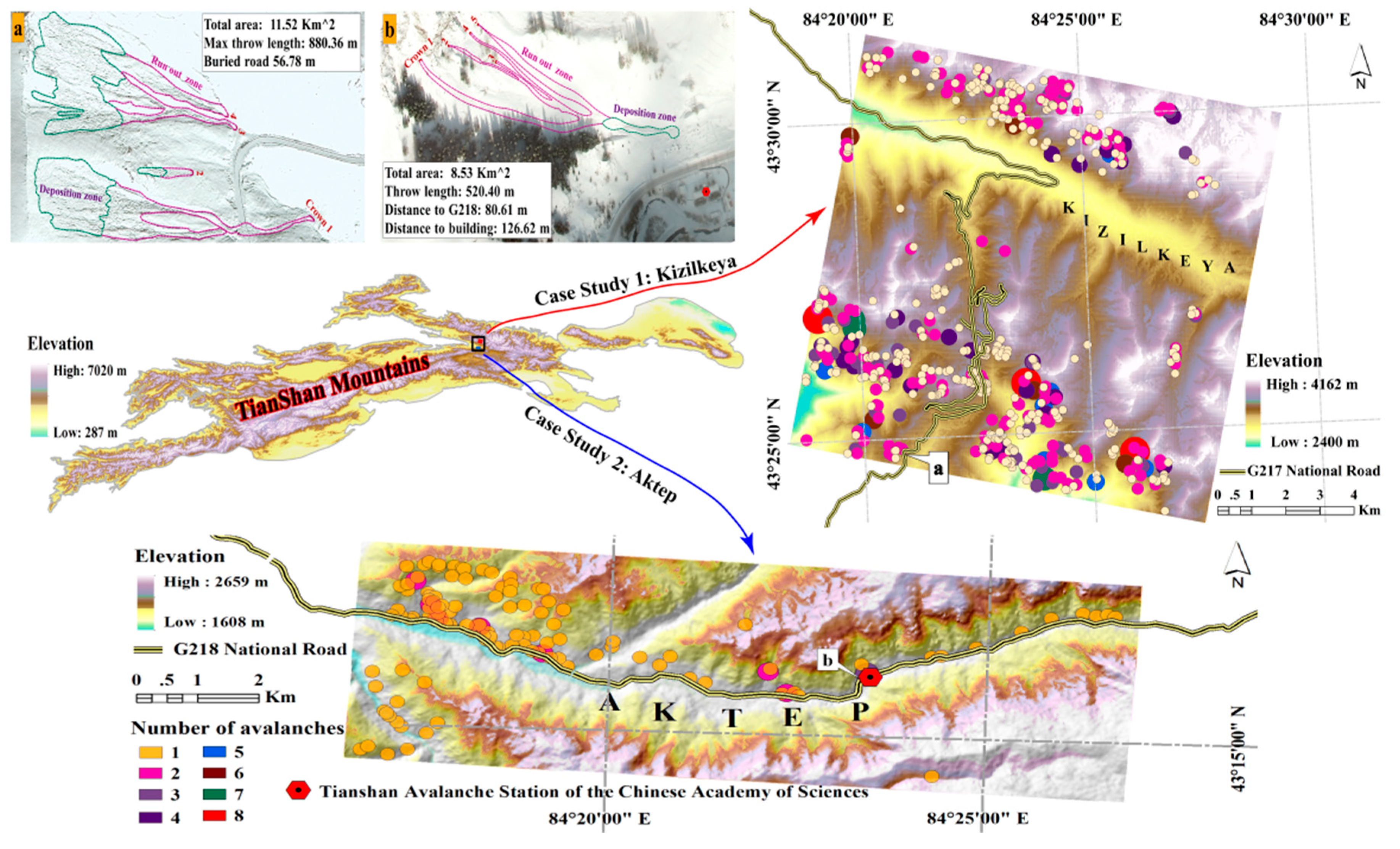
2. Study Site
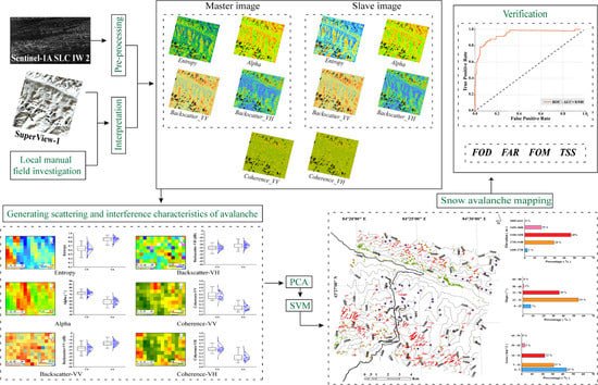
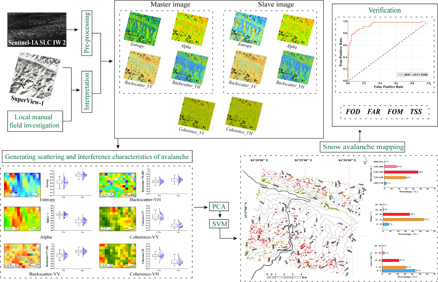
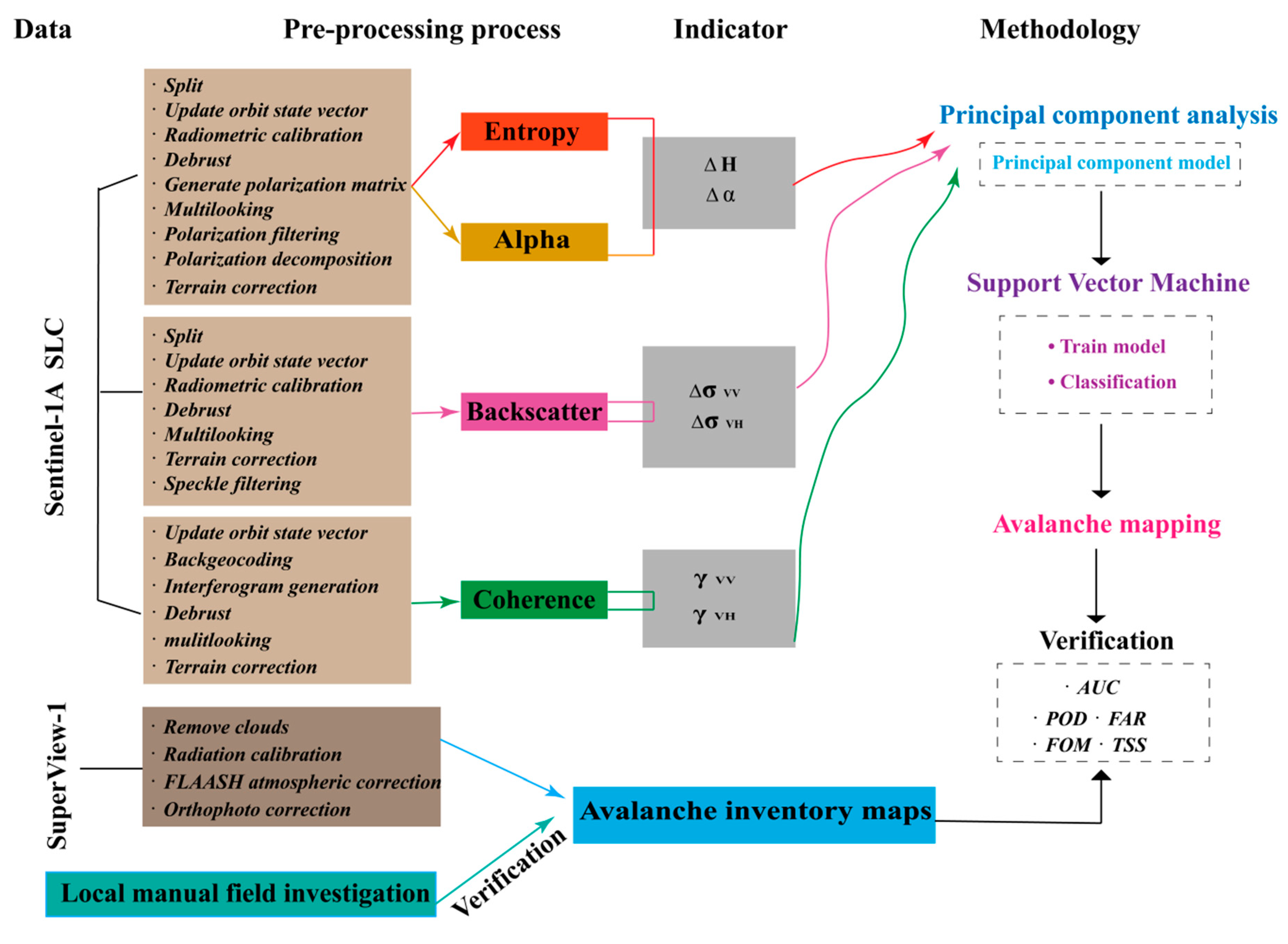
3. Materials and Methodology
3.1. Sentinel-1 Image Acquisition and Processing
- Split. The Sentinel-1A SLC image carries three sub-swath (IW1, IW2, IW3), while the study area is completely located in the IW2. Hence, only split IW2 for processing to reduce the computational burden;
- Orbital fine correction. Update the inaccurate information in the abstract meta data of the product with precision satellite position and velocity information which contained in POD (precise orbit determination) restituted orbit file;
- Radiation calibration. Typical SAR (synthetic aperture radar) data processing, which produces level-1 images, does not include radiometric corrections and significant radiometric bias remains. The significance of radiation correction is to make the pixel values of the SAR images truly represent the radar backscatter of the reflecting surface;
- Debrust. For the IW model SLC products, each sub-swath consists of a series of burst in azimuth. The individually focused complex burst data are included, in azimuth-time order, into a single sub-swath image, with black-fill demarcation in between. Debrust processing can eliminate black-fill demarcation by resampling and merging;
- Multilooking. Average the resolution of the range and azimuth direction of the image, suppress the speckle noise of the image and improve the radiation resolution of the image. Number of range looks: 4. Number of azimuth looks: 1;
- Range Doppler terrain correction. The topographical variations of the scene and the tilt of the satellite sensor may distort the distance in the SAR image. Terrain correction makes the geometric representation of the image as close as to the real world. Map projection: WGS84;
- Speckle filtering. The Lee sigma filter method is used to remove the noise in the Sentinel-1 image caused by the random superposition of multiple scattering sources in space. Filter: Lee sigma. Target window size: 3 × 3. Sigma: 0.9.
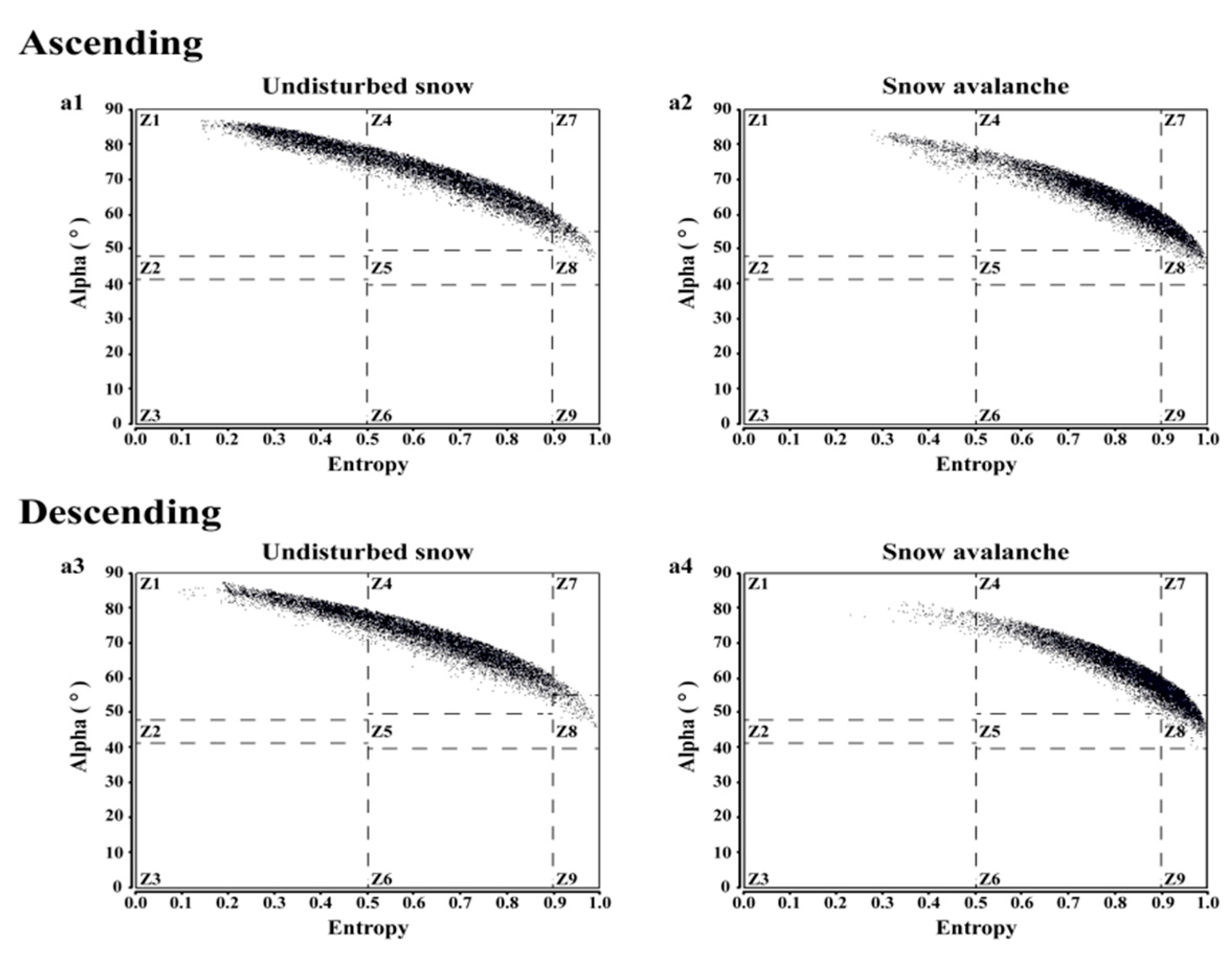
3.1.1. Generating Scattering Characteristics of Avalanche
3.1.2. Generating Interference Characteristics of Avalanche
3.2. SuperView-1 Image Collection and Processing
3.3. Local Manual Field Investigation
3.4. Methodology
3.4.1. Principal Component Analysis
- Perform Kaiser–Meyer–Olkin (KMO) and Bartlett spherical test on each index matrix [41]. Commonly used KMO metrics are given by Kaiser: above 0.9 = very suitable; 0.8 = suitable; 0.7 = moderate; 0.6 = not very suitable; below 0.5 = extremely unsuitable;
- Standardization brings all indicators to a common platform with a mean of zero and a standard deviation of one;
- Calculate the eigenvalues, corresponding eigenvectors, contribution rate and cumulative contribution rate of the covariance matrix. The component that satisfies the condition that the eigen value are greater than 1 and the cumulative contribution rate is more than 80% will be selected as the principal component [42];
- Calculate the rotated factor loadings of principal components (PCs) to obtain the linear combination of the principal components, thereby obtaining a comprehensive model.
3.4.2. Support Vector Machine
3.4.3. Model Evaluation
4. Results
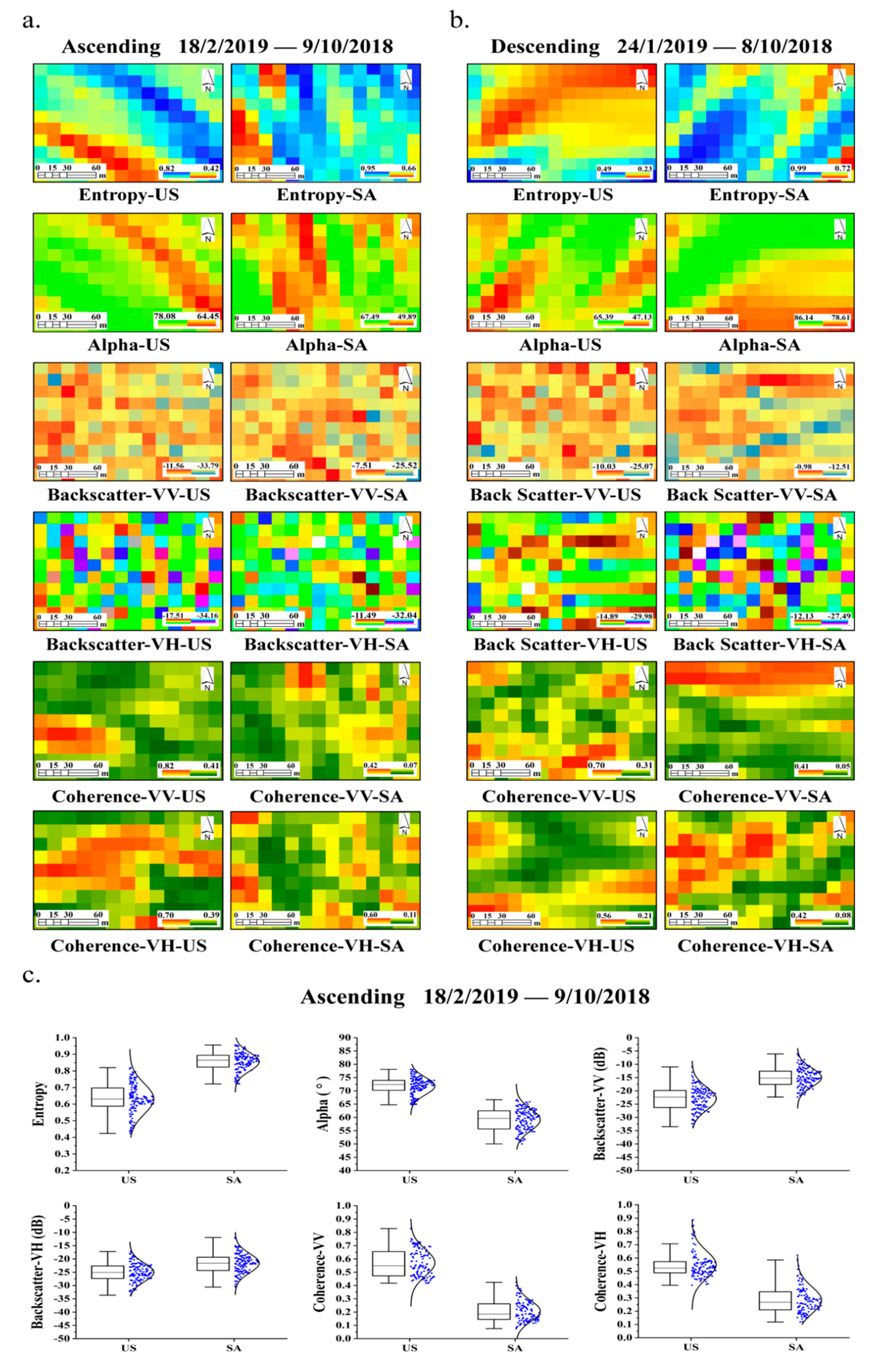
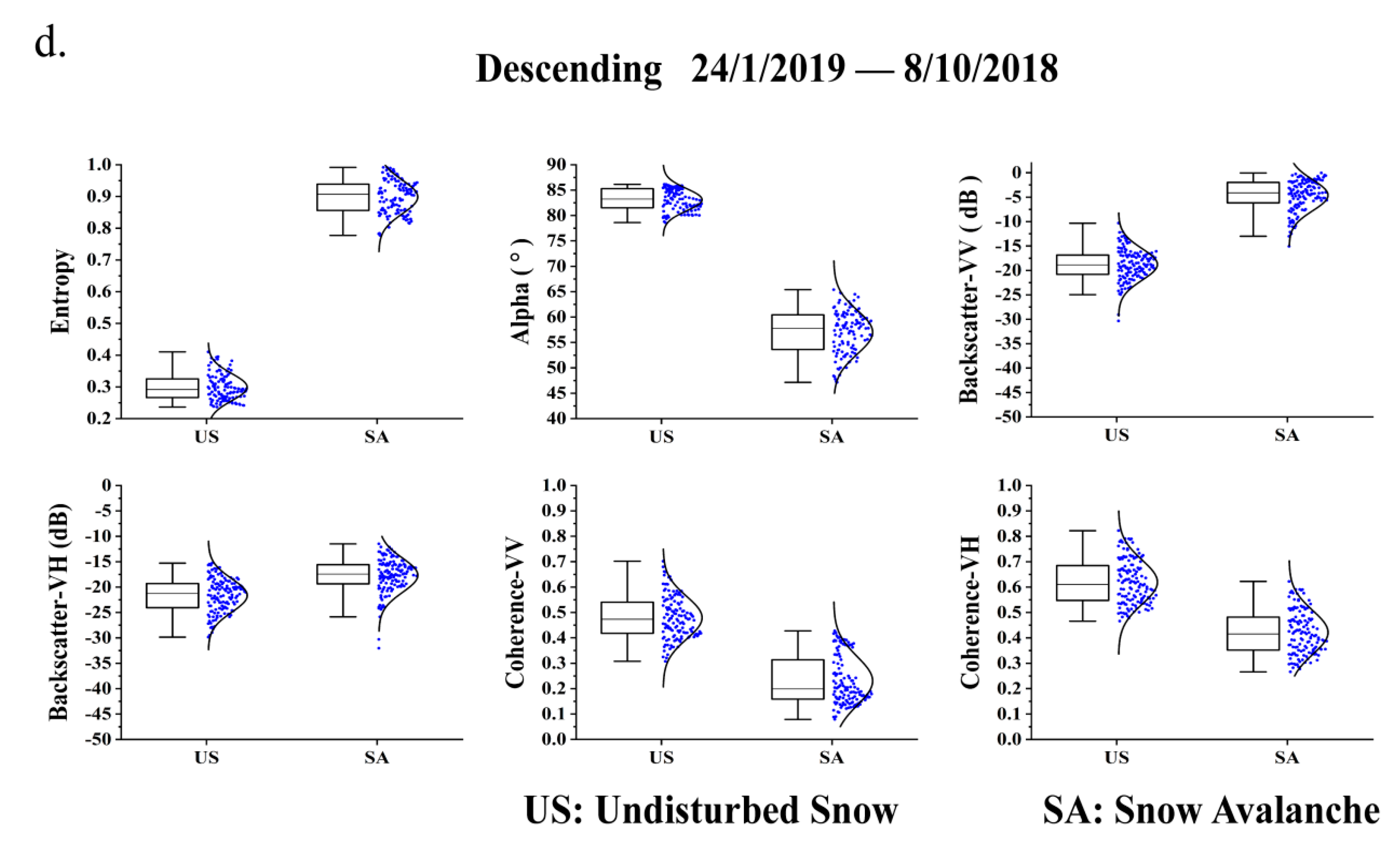
4.1. Characteristics from Sentinel-1 Images of Avalanches
4.2. Generating Characteristic Variables
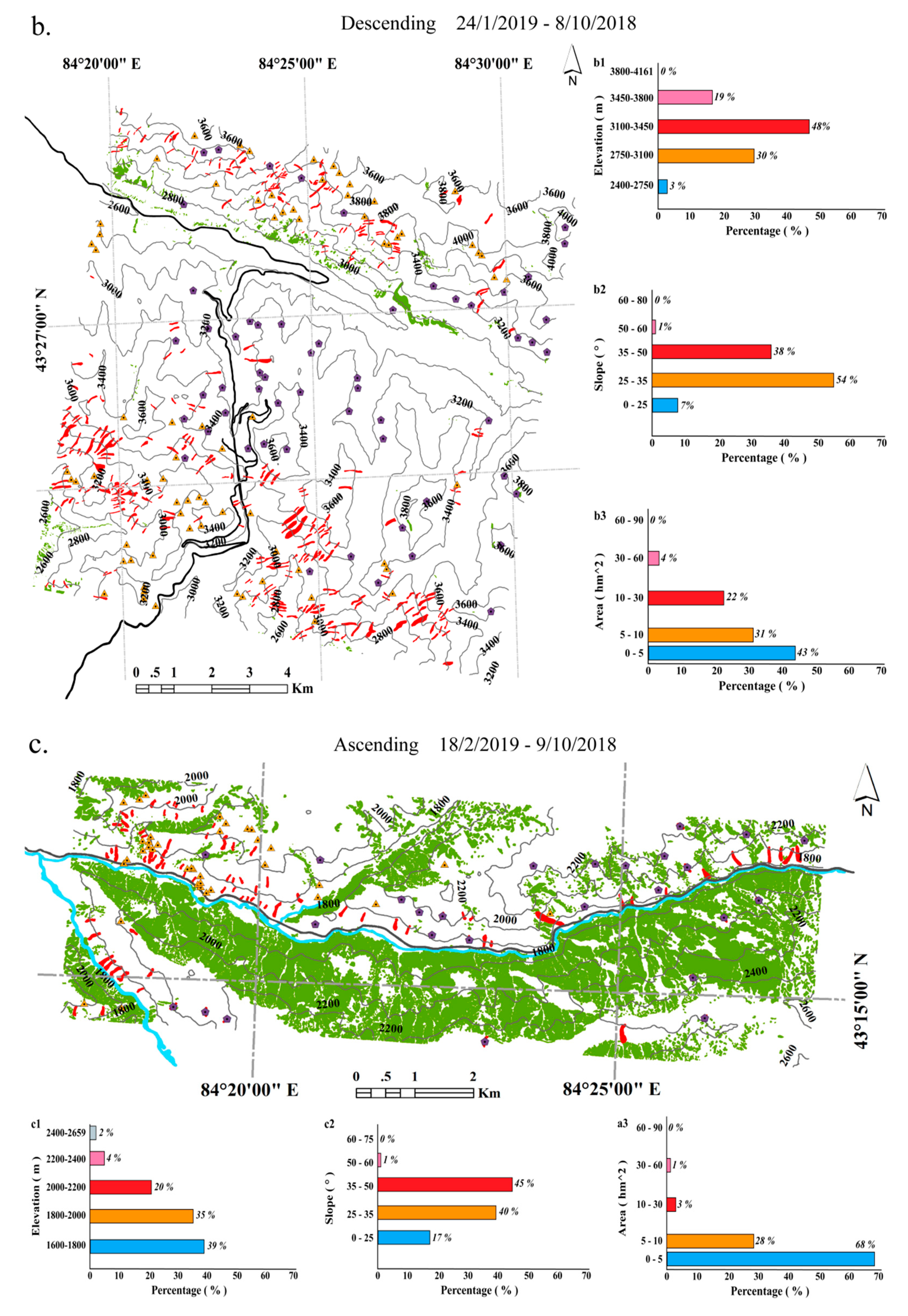
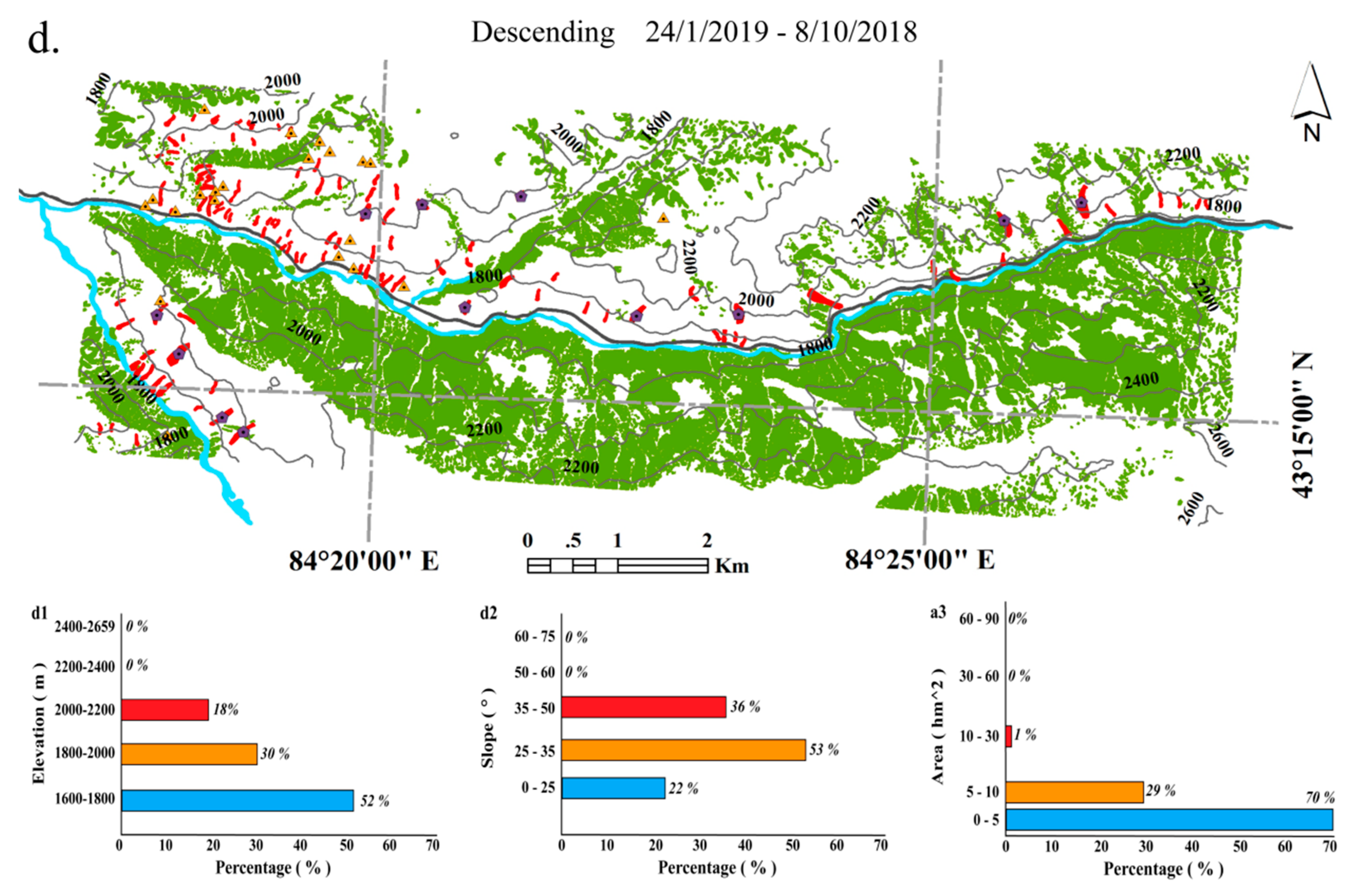
4.3. Snow Avalanche Mapping
4.3.1. Case Study 1: Kizilkeya
4.3.2. Case Study 2: Aktep
4.4. Verification
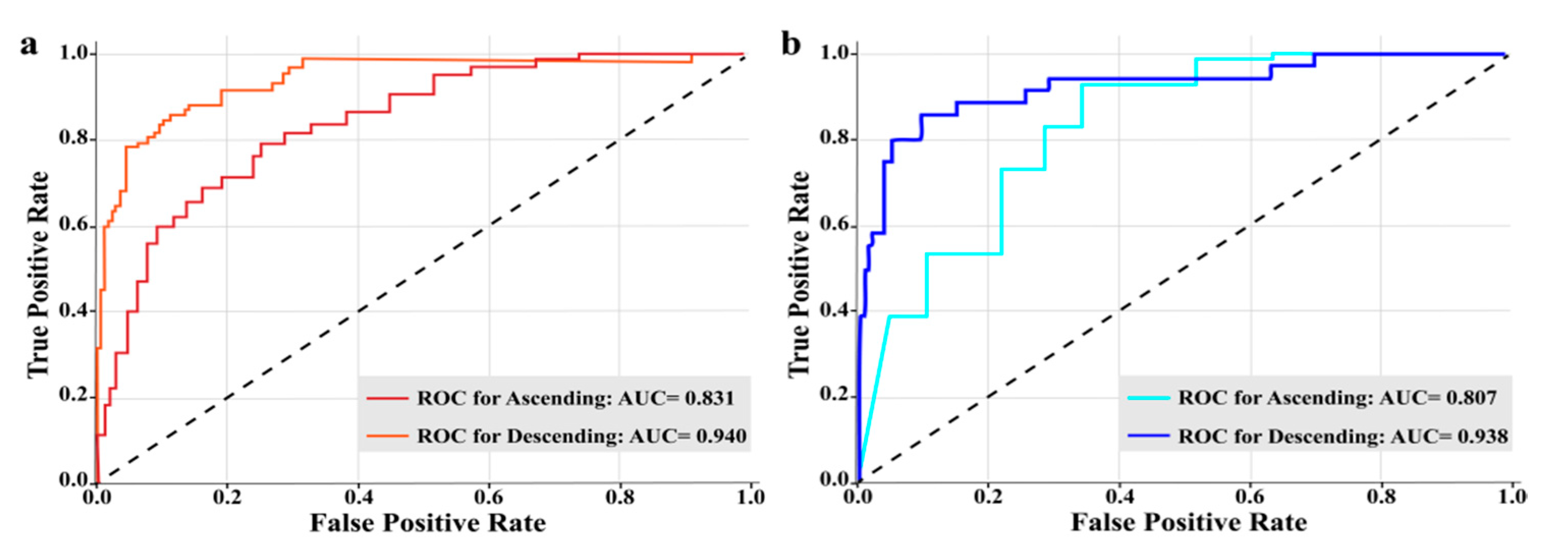
4.4.1. AUC
4.4.2. Statistical Indicator
5. Discussion
5.1. Impact of Source Image Availability
5.2. Performance of the Automatic Avalanche Detection Method
5.3. Sources of Error
5.4. Limitations and Future Development
6. Conclusions
Author Contributions
Funding
Acknowledgments
Conflicts of Interest
References
- Ballesteros-Cánovas, J.A.; Trappmann, D.; Madrigal-González, J.; Eckert, N.; Stoffel, M. Climate warming enhances snow avalanche risk in the Western Himalayas. Proc. Natl. Acad. Sci. USA 2018, 115, 3410–3415. [Google Scholar] [CrossRef] [PubMed]
- Grêt-Regamey, A.; Straub, D. Spatially explicit avalanche risk assessment linking Bayesian networks to a GIS. Nat. Hazards Earth Syst. Sci. 2006, 6, 911–926. [Google Scholar] [CrossRef]
- Blahut, J.; Klimeš, J.; Balek, J.; Hájek, P.; Červená, L.; Lysák, J. Snow avalanche hazard of the Krkonose National Park, Czech Republic. J. Maps 2017, 13, 86–90. [Google Scholar] [CrossRef]
- Krajick, K. Animals thrive in an avalanche’s wake. Science 1998, 279, 1853. [Google Scholar] [CrossRef]
- Gruber, U.; Bartelt, P. Snow avalanche hazard modelling of large areas using shallow water numerical methods and GIS. Environ. Model. Softw. 2007, 22, 1472–1481. [Google Scholar] [CrossRef]
- Gądek, B.; Kaczka, R.J.; Rączkowska, Z.; Rojan, E.; Casteller, A.; Bebi, P. Snow avalanche activity in Żleb Żandarmerii in a time of climate change (Tatra Mts., Poland). Catena 2017, 158, 201–212. [Google Scholar] [CrossRef]
- Bernardino, C.; Valerio, D.B.; Barbara, F. The influence of extreme snowfall on snow avalanche impact pressure. Contrib. Polit. Econ. 2013, 28, 1–22. [Google Scholar]
- Rudolf, M.F.; Sauermoser, S.; Mears, A.I. The Technical Avalanche Protection Handbook; Ernst & Sohn: Berlin, Germany, 2015; pp. 93–127. [Google Scholar]
- Germain, D. Snow avalanche hazard assessment and risk management in northern Quebec, eastern Canada. Nat. Hazards 2015, 80, 1303–1321. [Google Scholar] [CrossRef]
- Gaume, J.; Herwijnen, A.V.; Chambon, G.; Wever, N.; Schweizer, J. Snow fracture in relation to slab avalanche release: Critical state for the onset of crack propagation. Cryosphere 2017, 11, 217–228. [Google Scholar] [CrossRef]
- Eckerstorfer, M.; Malnes, E. Manual detection of snow avalanche debris using high-resolution Radarsat-2 SAR images. Cold Reg. Sci. Technol. 2015, 120, 205–218. [Google Scholar] [CrossRef]
- Singh, D.K.; Mishra, V.D.; Gusain, H.S.; Gupta, N.; Singh, A.K. Geo-spatial modeling for automated demarcation of snow avalanche hazard areas using Landsat-8 satellite images and in situ data. J. Indian Soc. Remote Sens. 2019, 47, 513–526. [Google Scholar] [CrossRef]
- Bedard, A.J. Low-frequency sound waves associated with avalanches, atmospheric turbulence, severe weather, and earthquakes. J. Acoust. Soc. Am. 1998, 94, 1872. [Google Scholar] [CrossRef]
- Chadha, A.; Satam, N. Snow Avalanche: Study and detection using remote sensing techniques. Int. J. Recent Trends Eng. Res. 2017, 3, 11–23. [Google Scholar]
- Luckman, B.H. Drop stones resulting from snow avalanche deposition on lake ice. J. Glaciol. 1975, 70, 186–188. [Google Scholar] [CrossRef]
- D’Aubeterre, G.D.B.; Favillier, A.; Mainieri, R.; Lopez, S.J.; Eckert, N.; Saulnier, M.; Peiry, J.L.; Stoffel, M.; Corona, C. Tree-ring reconstruction of snow avalanche activity: Does avalanche path selection matter? Sci. Total Environ. 2019, 684, 496–508. [Google Scholar]
- Bühler, Y.; Hafner, E.; Zweifel, B.; Zesiger, M.; Heisig, H. Where are the avalanches? Rapid mapping of a large snow avalanche period with optical satellites. Cryosph. Discuss. 2019, 119. [Google Scholar] [CrossRef]
- Lato, M.J.; Frauenfelder, R.; Bühler, Y. Automated detection of snow avalanche deposits: Segmentation and classification of optical remote sensing imagery. Nat. Hazards Earth Syst. Sci. 2012, 12, 2893–2906. [Google Scholar] [CrossRef]
- Wiesmann, A.; Wegmuller, U.; Honikel, M.; Strozzi, T.; Werner, C. Potential and methodology of satellite based SAR for hazard mapping. In Proceedings of the IEEE International Geoscience & Remote Sensing Symposium, Sydney, Australia, 9–13 July 2001. [Google Scholar]
- Eckerstorfer, M.; Vickers, H.; Malnes, E. Snow avalanche activity monitoring from space: Creating a complete avalanche activity dataset for a Norwegian forecasting region. In Proceedings of the International Snow Science Workshop, Breckenridge, CO, USA, 3–7 October 2016. [Google Scholar]
- Benz, U.; Baatz, M.; Schreier, G. OSCAR object oriented segmentation and classification of advanced radar allow automated information extraction. In Proceedings of the IEEE International Geoscience & Remote Sensing Symposium, Sydney, Australia, 9–13 July 2001. [Google Scholar]
- Malnes, E.; Eckerstorfer, M.; Vickers, H. First Sentinel-1 detections of avalanche debris. Cryosph. Discuss. 2015, 9, 1943–1963. [Google Scholar] [CrossRef]
- Eckerstorfer, M.; Malnes, E.; Frauenfelder, R.; Domass, U.; Brattlien, K. Avalanche debris detection using satellite-borne radar and optical remote sensing. In Proceedings of the International Snow Science Workshop, Banff, AB, Canada, 29 September–3 October 2014. [Google Scholar]
- Eckerstorfer, M.; Malnes, E.; Müller, K. A complete snow avalanche activity record from a Norwegian forecasting region using Sentinel-1 satellite-radar data. Cold Reg. Sci. Technol. 2017, 8, 39–51. [Google Scholar] [CrossRef]
- Singh, A.; Ganju, A. Artificial Neural Networks for snow avalanche forecasting in Indian Himalaya. In Proceedings of the 12th International Conference of International Association for Computer Methods and Advances in Geomechanics (IACMAG), Goa, India, 1–6 October 2008. [Google Scholar]
- Möhle, S.; Bründl, M.; Beierle, C. Modeling a system for decision support in snow avalanche warning using balanced random forest and weighted random forest. Bioinform. Res. Appl. 2014, 8722, 80–91. [Google Scholar]
- Rahmati, O.; Ghorbanzadeh, O.; Teimurian, T.; Mohammadi, F.; Tiefenbacher, J.P.; Falah, F.; Pirasteh, S.; Ngo, P.T.T.; Bui, D.T. Spatial modeling of snow avalanche using machine learning models and geo-environmental factors: Comparison of effectiveness in two mountain regions. Remote Sens. 2019, 11, 2995. [Google Scholar] [CrossRef]
- Abake, G.; Al-Hanbali, A.; Alsaaideh, B. Potential hazard map for snow disaster prevention using GIS-based weighted linear combination analysis and remote sensing techniques: A case study in Northern Xinjiang, China. Adv. Remote Sens. 2014, 3, 260–271. [Google Scholar] [CrossRef][Green Version]
- Qiu, J.Q. Avalanche; Xinjiang Science and Technology Press: Urumqi, China, 2004; pp. 182–186. [Google Scholar]
- Osamu, A.; Li, L.H.; Bai, L.; Hao, J.S.; Hirashima, H.; Xu, J.R. Characteristics of avalanche release and an approache of avalanche forecasting system using SNOW PACK model in the Tianshan mountains, China. In Proceedings of the International Snow Science Workshop, Breckenridge, CO, USA, 2 October 2016. [Google Scholar]
- Hao, J.H.; Huang, F.R.; Liu, Y.; Amanambu, A.C.; Li, L.H. Avalanche activity and characteristics of its triggering factors in the western Tianshan Mountains, China. J. Mt. Sci. 2018, 15, 1397–1411. [Google Scholar] [CrossRef]
- Liu, D.X.; Cheng, Z.L.; Zhao, X.; Huang, J.H.; Liu, J.K. Research and application status of avalanche prevention and control engineering. J. Mt. 2013, 31, 425–433. [Google Scholar]
- Heffernan, O. Coming down the tracks. Nat. Clim. Chang. 2018, 8, 937–939. [Google Scholar] [CrossRef]
- Banque, X.; Lopezsanchez, J.M.; Monells, D.; Ballester, D.; Duro, J.; Koudogbo, F. Polarimetry based land cover classification with Sentinel-1 data. In Proceedings of the PolInSAR 2015, Frascati, Italy, 26–30 January 2015. [Google Scholar]
- Xie, Q.X.; Meng, Q.Y.; Zhang, L.L.; Wang, C.M.; Wang, Q.; Zhao, S.H. Combining of the H/A/Alpha and Freeman–Durden polarization decomposition methods for soil moisture retrieval from full-polarization Radarsat-2 data. Adv. Meteorol. 2018, 2018, 9436438. [Google Scholar] [CrossRef]
- Ulaby, F.T.; Moore, R.K.; Funk, A.K. Microwave Remote Sensing, Active and Passive: From Theory to Applications; Artech House: Norwood, MA, USA, 1986; pp. 2026–2086. [Google Scholar]
- Li, Z.; Guo, H.D.; Li, X.W.; Wang, C.L. SAR interferometry coherence analysis and snow mapping. J. Remote Sens. 2002, 6, 334–338. [Google Scholar]
- Tanase, M.A.; Santoro, M.; Wegmüller, U. Properties of X, C and L-band repeat pass interferometric SAR coherence in Mediterranean pine forests affected by fires. Remote Sens. Environ. 2010, 114, 2182–2194. [Google Scholar] [CrossRef]
- Clark, N.R.; Ma’Ayan, A. Introduction to statistical methods to analyze large data sets: Principal Components Analysis. Sci. Signal. 2011, 4. [Google Scholar] [CrossRef]
- Tripathi, M.; Singal, S.K. Use of Principal Component Analysis for parameter selection for development of a novel Water Quality Index: A case study of river Ganga India. Ecol. Indic. 2019, 96, 430–436. [Google Scholar] [CrossRef]
- Li, F.; Huang, J.H.; Zeng, G.M.; Yuan, X.Z.; Li, X.D.; Liang, J.; Wang, X.Y.; Tang, X.J.; Bai, B. Spatial risk assessment and sources identification of heavy metals in surface sediments from the Dongting Lake, Middle China. J. Geochem. Explor. 2013, 132, 75–83. [Google Scholar] [CrossRef]
- Xiao, M.H.; Ma, Y.; Feng, Z.X.; Deng, Z.; Hou, S.S.; Shu, L.; Lu, Z.X. Rice blast recognition based on principal component analysis and neural network. Comput. Electron. Agric. 2018, 154, 482–490. [Google Scholar] [CrossRef]
- Chauhan, V.K.; Dahiya, K.; Sharma, A. Problem formulations and solvers in linear SVM: A review. Artif. Intell. Rev. 2018, 52, 803–855. [Google Scholar] [CrossRef]
- Marjanovis, M.; KovacEvic, M.; Bajat, B.; Voženílek, V. Landslide susceptibility assessment using SVM machine learning algorithm. Eng. Geol. 2011, 123, 225–234. [Google Scholar] [CrossRef]
- Alham, N.K.; Li, M.; Liu, Y.; Ponraj, M.; Qi, M. A distributed SVM ensemble for image classification and annotation. In Proceedings of the 9th International Conference on Fuzzy Systems and Knowledge Discovery, SiChuan, China, 29–31 May 2012. [Google Scholar]
- Wesselink, D.S.; Malnes, E.; Eckerstorfer, M.; Lindenbergh, R.C. Automatic detection of snow avalanche debris in central Svalbard using C-band SAR data. Polar Res. 2017, 36. [Google Scholar] [CrossRef][Green Version]
- Eckerstorfer, M.; Vickers, H.; Malnes, E.; Grahn, J. Near-Real time automatic snow avalanche activity monitoring system using Sentinel-1 SAR data in Norway. Remote Sens. 2019, 11, 2863. [Google Scholar] [CrossRef]
- Korzeniowska, K.; Bühler, Y.; Marty, M.; Korup, O. Regional snow avalanche detection using object-based image analysis of near-infrared aerial imagery. Nat. Hazards Earth Syst. Sci. 2017, 17, 1823–1836. [Google Scholar] [CrossRef]
- Vickers, H.; Eckerstorfer, M.; Malnes, E.; Larsen, Y.; Hindberg, H. A method for automated snow avalanche debris detection through use of Synthetic Aperture Radar (SAR) imaging: Automated avalanche detection. Earth Space Sci. 2016, 3, 446–462. [Google Scholar] [CrossRef]


| Characteristic | Kizilkeya | Aktep |
|---|---|---|
| Area | 150.08 km2 | 54.74 km2 |
| Elevation | 2400–4162 m | 1608–2659 m |
| Snowline | 3700 m | 3000 m |
| Forest line | 2400 m | 2800 m |
| Snow type | Continental dry cold snow | |
| Multiyear stable snow days | 187 d | 180 d |
| Average precipitation | 339 mm/year | 312 mm/year |
| Slope range | 0°–79.31° | 0°–74.08° |
| Number of avalanche paths | 681 | 172 |
| Avalanche type | trench-type, slope-type, groove-slope-type, slab avalanches | trench-type, slope-type, groove-slope-type |
| Characteristic. | Ascending | Descending | ||
|---|---|---|---|---|
| Dates | 18 February 2019 | 9 October 2018 | 24 January 2019 | 8 October 2018 |
| Slave/master | Master | Slave | Master | Slave |
| Track | 12 | 165 | ||
| Width | 250 km | |||
| Ground resolution | 5 × 20 m | |||
| Baseline | 124.536 m | 79.657 m | ||
| Characteristic | Kizilkeya | Aktep | |
|---|---|---|---|
| Revisit period | 1 d | ||
| Resolution | multispectral | 2 m | |
| panchromatic | 0.5 m | ||
| Orbit height | 530 km | ||
| Width | 12 km | ||
| Side swing angle | 0.56° | ||
| Maximum image size | 60 × 70 km | ||
| Cloud content | 1.2% | 0.5% | |
| KMO Sampling Suitability | Bartlett Sphericity Test | ||||
|---|---|---|---|---|---|
| Approximate Chi-Squared | Degrees of Freedom | Significance | |||
| Kizilkeya | Ascending | 0.824 | 461.164 | 21 | 0.000 |
| Descending | 0.871 | 973.434 | 10 | 0.000 | |
| Aktep | Ascending | 0.707 | 131.354 | 36 | 0.000 |
| Descending | 0.747 | 129.047 | 28 | 0.000 | |
| Components | Kizilkeya | Aktep | ||||||
|---|---|---|---|---|---|---|---|---|
| Ascending | Descending | Ascending | Descending | |||||
| Eigen Values | Cumulative Variance | Eigen Values | Cumulative Variance | Eigen Values | Cumulative Variance | Eigen Values | Cumulative Variance | |
| 1 | 3.436 | 57.26% | 2.720 | 45.33% | 3.383 | 56.38% | 2.531 | 42.18% |
| 2 | 1.580 | 88.86% | 1.690 | 73.51% | 1.538 | 82.01% | 1.640 | 69.52% |
| 3 | 0.575 | 93.18% | 1.087 | 91.62% | 0.959 | 97.99% | 1.089 | 87.67% |
| 4 | 0.235 | 97.10% | 0.310 | 96.77% | 0.091 | 99.51% | 0.610 | 97.83% |
| 5 | 0.141 | 99.45% | 0.185 | 99.85% | 0.030 | 100.00% | 0.126 | 99.93% |
| 6 | 0.033 | 100.00% | 0.008 | 100.00% | 0.000 | 100.00% | 0.004 | 100.00% |
| Indicators | Kizilkeya | Aktep | ||||||||
|---|---|---|---|---|---|---|---|---|---|---|
| Ascending | Descending | Ascending | Descending | |||||||
| PC1 | PC2 | PC1 | PC2 | PC3 | PC1 | PC2 | PC1 | PC2 | PC3 | |
| ΔH | 0.660 | 0.366 | 0.824 | −0.002 | −0.120 | 0.825 | 0.469 | 0.962 | 0.158 | −0.065 |
| Δα | 0.828 | −0.420 | 0.776 | 0.566 | 0.150 | −0.068 | 0.482 | −0.811 | 0.223 | −0.025 |
| ΔσVV | 0.948 | -0.174 | −0.871 | 0.344 | 0.127 | 0.785 | 0.616 | 0.088 | 0.266 | 0.960 |
| ΔσVH | 0.807 | 0.361 | 0.196 | 0.905 | 0.332 | 0.975 | 0.035 | 0.858 | 0.461 | −0.097 |
| γVV | −0.425 | 0.797 | −0.780 | 0.266 | 0.143 | 0.690 | −0.666 | −0.451 | 0.826 | −0.086 |
| γVH | −0.763 | −0.418 | 0.180 | −0.602 | 0.777 | 0.808 | −0.511 | −0.019 | 0.949 | −0.131 |
| Statistics | Evaluation Index | |||||||
|---|---|---|---|---|---|---|---|---|
| Kizilkeya | Aktep | |||||||
| POD | FAR | FOM | TSS | POD | FAR | FOM | TSS | |
| Ascending | 0.754 | 0.139 | 0.246 | 0.751 | 0.897 | 0.109 | 0.103 | 0.890 |
| Descending | 0.820 | 0.116 | 0.180 | 0.818 | 0.924 | 0.340 | 0.076 | 0.921 |
© 2020 by the authors. Licensee MDPI, Basel, Switzerland. This article is an open access article distributed under the terms and conditions of the Creative Commons Attribution (CC BY) license (http://creativecommons.org/licenses/by/4.0/).
Share and Cite
Yang, J.; Li, C.; Li, L.; Ding, J.; Zhang, R.; Han, T.; Liu, Y. Automatic Detection of Regional Snow Avalanches with Scattering and Interference of C-band SAR Data. Remote Sens. 2020, 12, 2781. https://doi.org/10.3390/rs12172781
Yang J, Li C, Li L, Ding J, Zhang R, Han T, Liu Y. Automatic Detection of Regional Snow Avalanches with Scattering and Interference of C-band SAR Data. Remote Sensing. 2020; 12(17):2781. https://doi.org/10.3390/rs12172781
Chicago/Turabian StyleYang, Jinming, Chengzhi Li, Lanhai Li, Jianli Ding, Run Zhang, Tao Han, and Yang Liu. 2020. "Automatic Detection of Regional Snow Avalanches with Scattering and Interference of C-band SAR Data" Remote Sensing 12, no. 17: 2781. https://doi.org/10.3390/rs12172781
APA StyleYang, J., Li, C., Li, L., Ding, J., Zhang, R., Han, T., & Liu, Y. (2020). Automatic Detection of Regional Snow Avalanches with Scattering and Interference of C-band SAR Data. Remote Sensing, 12(17), 2781. https://doi.org/10.3390/rs12172781