Abstract
A low-mass and low-volume dual-polarization L-band radiometer is introduced that has applications for ground-based remote sensing or unmanned aerial vehicle (UAV)-based mapping. With prominent use aboard the ESA Soil Moisture and Ocean Salinity (SMOS) and NASA Soil Moisture Active Passive (SMAP) satellites, L-band radiometry can be used to retrieve environmental parameters, including soil moisture, sea surface salinity, snow liquid water content, snow density, vegetation optical depth, etc. The design and testing of the air-gapped patch array antenna is introduced and is shown to provide a 3-dB full power beamwidth of 37°. We present the radio-frequency (RF) front end design, which uses direct detection architecture and a square-law power detector. Calibration is performed using two internal references, including a matched resistive source (RS) at ambient temperature and an active cold source (ACS). The radio-frequency (RF) front end does not require temperature stabilization, due to characterization of the ACS noise temperature by sky measurements. The ACS characterization procedure is presented. The noise equivalent delta (Δ) temperature (NEΔT) of the radiometer is ~0.14 K at 1 s integration time. The total antenna temperature uncertainty ranges from 0.6 to 1.5 K.
Keywords:
microwave; radiometer; L-band; low-mass; patch array; patch antenna; UAV; soil moisture; passive 1. Introduction
The modern age of space-borne L-band (1–2 GHz) microwave radiometers began with the European Space Agency (ESA) Soil Moisture and Ocean Salinity Satellite (SMOS) [1] in 2010. This was followed by the National Aeronautics and Space Administration (NASA) satellites Aquarius [2] and Soil Moisture Active Passive (SMAP) [3]. L-band radiometry typically occurs in the protected frequency band from 1400–1427 MHz. Retrievals of environmental state parameters, such as soil moisture [4,5], sea surface salinity [6], vegetation optical depth [7,8], snow liquid water [9], snow density [10,11,12], soil freeze/thaw [13,14], and sea ice thickness [15], have all been demonstrated, based on dual-polarization microwave brightness temperatures in this band.
Near-surface L-band radiometry, such as with the Portable L-band Radiometer (PoLRa), allows L-band radiometry at high spatial resolution from a number of platforms. The compact and low-mass design allows use on unmanned aerial vehicles (UAVs) or drones, wheeled vehicles, or fixed on towers, poles, or buildings. The drone-mounted PoLRa is capable of providing ground resolution of a few meters (<10 m).
UAV-based L-band radiometers have been demonstrated previously in [16,17]. Neither of these systems provide dual-polarization off-nadir antenna temperatures which are optimal for use with established retrieval algorithms such as the Tau-Omega (TO) [18,19] or Two-Stream (2S) emission models (EMs) [5]. The PoLRa is a direct-detection radiometer providing calibrated dual-polarization L-band antenna temperatures with resolution of ~0.14 K at 1 s integration, and total uncertainty ranging between 0.6–1.5 K, depending on integration time and input antenna temperature. PoLRa uses a unique dual 2 × 2 patch array antenna with an air-gap substrate for high gain and low Ohmic losses. A unique antenna temperature correction scheme allows correction for the relatively wide antenna power full beamwidth of 37° at −3 dB sensitivity. The correction convolves the antenna pattern with modeled angular dependent brightness temperatures of facets, while also considering polarization mixing introduced by nature of the geometry at large angles off of boresight (see Appendix in [20]). PoLRa is a research-ready radiometer system, and its characterization is demonstrated herein.
The following sections present the radiometer hardware, its characterization, initial results, and then conclusions. Hardware includes the radiometer electronics and antenna. Characterization includes the radiometer resolution and stability, calibration, and uncertainty. Initial results include drone-based antenna temperature measurements and soil moisture retrievals.
2. Hardware
The following subsections introduce the PoLRa hardware, including the radio-frequency (RF) front end, the back end, and the antenna.
2.1. RF Front End
PoLRa is a direct-detection radiometer with three analog filter stages, including one before the first amplifier. The front-end filter is critical for preventing radio-frequency inference (RFI) signals from saturating the low noise amplifier (LNA) [21]. The radiometer uses two internal calibration noise sources as references, including a matched resistive source (RS) at ambient temperature, and an active cold source (ACS). A four-port low-loss RF switch switches between the two calibration sources and the two (vertical and horizontal) polarization antennas. Temperature sensors monitor the physical temperatures of the reference noise sources, as well as the antenna and cable. After multiple filter-amplifier stages, the RF signal is detected by a linear square-law power detector.
The block diagram of the RF front end is shown in Figure 1. The filters are ceramic resonator filters, the two LNA stages provide a total gain of ~70 dB. The RF components are currently connected with coaxial cable lines and SubMiniature version A (SMA)-type connectors. The RF components could alternatively be connected with microstrips or coplanar waveguides, which allows the implementation of the entire RF front end on a single printed circuit board (PCB). The measured response of a single bandpass filter is shown in Figure 2.

Figure 1.
Block diagram of the L-band radiometer radio-frequency (RF) front end and post-detection electronics.
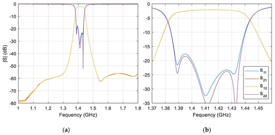
Figure 2.
Filter response measured with vector network analyzer (VNA): (a) broadband response; (b) frequenc y-axis zoomed near the protected band.
The front-end loss, or noise figure (NF), is driven by the components before the first LNA, and determines the radiometer system noise temperature, and thus the radiometric resolution. Due to the required low-mass and -volume of PoLRa, the use of a large low-loss resonant cavity filter is impractical. The insertion loss of the four port RF switch, the isolator, and the ceramic cavity filter are 1.3 dB, 0.2 dB, and 2.1 dB, respectively. The NF of the first LNA is 0.6 dB, and there is an additional loss due to all connectors and SMA sections of ~0.8 dB. The NF from the switch through, and including, the first LNA is 5.0 dB. The radiometer system noise temperature is calculated from the NF in dB using [22]:
where is 290 K. This corresponds to of 627 K.
2.2. Back End and Processing
The Linux microcontroller drives the switch, reads the temperature sensors, and samples the analog to digital converter (ADC), reading the power detector output signal. The switch has a settling time of less than 1 ms, and typically a full calibration cycle takes ~69 ms, with 16 ms spent integrating each switch position, and the four temperature sensors are sampled during the four ~1 ms switch position settling periods. The ADC is sampled at ~2 kHz and 22 bits, and the RC time constant of the low pass filter is ms. The ADC is capable of detecting <0.01 mV resolution, due to stable voltage regulation of the battery power source.
The radiometer runs entirely on 5V DC, and consumes ~0.7 A for a total of less than 4 W power consumption. The radiometer has no active temperature control, which was shown to be unnecessary to achieve the desired accuracies comparable to satellite-borne L-band radiometers. Instead, we rely on characterization of the physical-temperature dependence of the ACS. This characterization is presented in detail in Section 3.1. The calibration procedure of radiometer noise temperatures is also presented in Section 3.
2.3. Antenna Design and Characterization
The unique dual patch array antenna is both compact and lightweight, and provides sufficient directivity to obtain reasonable ground resolution, low back-lobe contribution, and small polarization crosstalk. The printed circuit board (PCB) patch arrays use two PCB layers separated by an air gap to obtain high gain and high radiation efficiency. The patches are fed with uniform magnitude and phase from a microstrip feed network printed on the same PCB as the patches. The microstrip feed network is fed with a coaxial probe and connected to the front-end switch with a 1 m SMA cable. The antenna consists of two FR4 PCBs of 1.5 mm thickness, spaced with 6 mm PTFE spacers. The PCBs are attached using nylon screws running through the spacers and PCB layers. The total dimensions of the antenna are 0.6 m × 0.3 m × 9 mm.
The physical temperature of the antenna and the feed cables are monitored, as indicated in Figure 1. The antenna Ohmic losses and the loss of the coaxial feed cables are determined empirically as part of the ACS characterization described in Section 3. Figure 3 shows photographs of the antenna during ground-based sky measurements and during drone-based measurement.
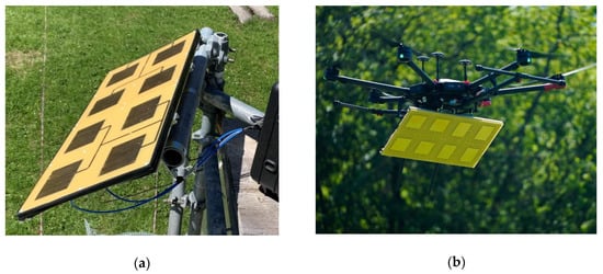
Figure 3.
Patch array antenna (a) mounted on tower during sky measurement; (b) mounted on multi-copter drone during flight measurements.
The return loss of the antenna was simulated using commercial finite-element electromagnetics software (ANSYS Electromagnetics Suite) during the design process. The feed network and patch dimensions were optimized to reduce the simulated return loss. The return loss was measured with a vector network analyzer (VNA) while the antenna was pointed towards the sky. The resonance of the antenna, or the minimum in return loss, is highly sensitive to the electromagnetic permittivity of the FR4 substrate. The final presented design required a number of iterations to accurately determine the FR4 permittivity supplied by the particular PCB vendor.
The angular-dependent power sensitivity pattern of the antenna was simulated with ANSYS Electromagnetics Suite finite element software. Additionally, the antenna power sensitivity pattern was measured using the solar overpass method described in [23]. The antenna was positioned such that the boresight pointed towards the azimuth and elevation angle of the highest solar zenith angle on that day. The relative antenna pattern measured with the solar overpass method characterizes the gain as a function of the total angle between the sun and the antenna boresight direction. The spherical polar angle will only exactly equal when the sun passes directly overhead, but the response with respect to should be between slices of constant . The solar overpass data are only shown through the −6 dB power level, because at high angles the horizon became cluttered by trees, and the measurements became unreliable. Figure 4 shows (a) the simulated and measured antenna return loss, and (b) the simulated and measured antenna power sensitivity pattern (normalized antenna gain).
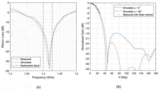
Figure 4.
(a) Antenna return loss from finite element simulation and VNA measurement; (b) normalized antenna power sensitivity pattern from finite element simulation and solar overpass measurement.
3. Radiometer Characterization
The following subsections describe the experimental characterization of the PoLRa radiometer. First, the active cold source (ACS) characterization procedure is described; second, stability and radiometric resolution are discussed; and third, the radiometer uncertainty quantification is presented.
3.1. Active Cold Source Characterization
Using an active cold source (ACS) with the radiometer hardware that is not temperature-stabilized requires determination of the temperature dependence of the ACS noise temperature. L-band brightness temperature of the sky is on the order of several Kelvin [24], depending on the Zenith angle, and in the absence of galactic background radiation. Galactic radiation has been shown to have up to 5 K or more impact on sky brightness temperatures [25], but this is reduced to less than 2 K by the relatively large 37° antenna beamwidth, compared to the 10° antenna assumed in [25].
The noise temperature at the switch inputs of the two polarizations, , can be expressed as the following expression:
where is the absorption of the total transmission path (TP) at the mean antenna/cable physical temperature (assuming that all antenna elements and cables are at uniform temperature). Note that the bar accent on temperature symbols refers to physical temperatures throughout the following discussion. in decibels (dB) is the cumulated loss between the antenna and the radiometer input (the mentioned TP) that accounts for losses due to the non-ideal antenna efficiency, cable loss, adapter and connector losses, and mismatch errors. We consider different losses in each polarization , due to respective variability in the cable and antenna losses of the two transmission paths (TPs).
We use the sky and ambient matched resistive source (RS) measurements to perform a two-point calibration of the radiometer with the switch inputs as the reference plane. The radiometer gain and the radiometer inherent offset (off) noise temperature are given by:
where is the noise temperature of the RS, which is equivalent to its physical temperature if the RS is perfectly matched. is the measured detector voltage for the RS switch position, and is the measured detector voltage for the switch positions at the antenna polarizations , while the antenna is directed towards the sky. The calibrated noise temperature of the ACS at the input of the switch is thus:
The noise temperature of an ACS reference is expected to be linearly increasing with its physical temperature, as demonstrated in [26,27]. Accordingly, the following linear model is applicable to express the ACS noise temperature as a function of its measured physical temperature ,
where and are the slope (units of K/K) and offset (units of K) of a linear least-squares regression, respectively. Given an ideal switch, because all values are referenced to the switch inputs, there is no polarization dependence on ACS noise temperature, meaning that . We use this along with the assumed linearity between ACS noise and physical temperature to formulate a cost function (CF) to minimize and obtain the losses and by least squares fit:
where and are the ACS noise temperatures derived from Equation (5), and using voltages available from sky measurements . The first term in the CF enforces the linearity of ACS noise with its physical temperature, and the second term enforces . The CF is minimized using a numerical global minimum finder to obtain optimal and . For an ideal measurement system, the resulting linear fit parameters used in Equation (6) would be identical for , but this is not the case in practice. To obtain the optimal polarization-independent linear temperature dependence of the ACS, the linear fit parameters and can be averaged over the two polarizations, which is equivalent to a linear fit of all values versus .
Figure 3a shows the setup for these sky measurements at the Davos-Laret Remote Sensing Field Laboratory [28]. The antenna was oriented towards the south with approximately 70° altitude angle. Sky measurements were performed at 5-min intervals over an approximately 11-h period between 7 and 8 May 2020. Evening to nighttime (17:00–06:00 local time) measurements were used in order to maximize the range of physical temperatures while also avoiding solar intrusion into the antenna. Potential galactic noise intrusion was also investigated using a night sky calculator, and estimated from our equatorial coordinates to be less than 1 K [25], with the worst case occurring at the beginning of the measurement period. Figure 5 shows the physical temperatures and the measured detector voltages. The evening cooling period provided a ~25 K temperature variation. Note that the detector on the PoLRa is an inverse slope detector, so lower voltages correspond to higher absolute power levels. Figure 6 provides the calibrated cold load brightness temperatures versus the ACS physical temperature along with the linear fit line over both polarizations and the 95% confidence interval of this fit line. Table 1 shows the parameter values resulting from the cost function (CF) minimization procedure.

Figure 5.
(a) Measured physical temperatures, and (b) raw voltages from detector measured during sky measurement versus time of day.
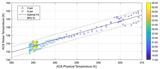
Figure 6.
Measured physical temperature of the active cold source (ACS) versus calibrated ACS noise temperature , and linear fit , for sky-measurement-based characterization of the ACS. The dotted line shows the 95% confidence interval (CI) of the linear model. The color bar indicates the local time at which each measurement was taken between 7 and 8 May 2020.

Table 1.
Parameter values from ACS characterization.
3.2. Radiometer Stability
For nominal use of the radiometer, the antenna temperatures at horizontal and vertical polarization are calibrated using a two-point calibration with internal matched resistive source (RS) and active cold source (ACS) as references. Similar to Equations (3) and (4), the radiometer gain and offset are calculated by:
and the noise temperature (at the input reference plane of the switch), for switch positions is given as:
where is the detector voltage measured for the switch at the horizontal and vertical polarization input ports while the antenna is pointing towards the target scene.
The radiometer stability was characterized by attaching resistive matched sources to the end of the two antenna feed cables. The radiometer was constantly measuring, beginning from cold startup, for about 20 min, using the 16 ms integration time on each of the two external resistive sources. The corresponding total time to switch between the four switch positions, sample the detector for 16 ms at each position (ACS, RS, and the two external resistive sources), and sample the four temperature sensors is 69 ms. During the stability test, the radiometer was operated on battery power.
The external matched resistive sources were passively maintained at ambient temperature during the stability test. The respective RF cables and the matched resistive sources are assumed to be at equal and uniform temperature. A thermocouple temperature sensor was attached to the matched resistive sources to monitor their physical temperature during the test. A slight heating (~0.6 K) of the matched resistive sources during the measurement period was detected, likely caused by heat generated by the radiometer electronics, which were in close proximity.
The noise equivalent delta (Δ) temperature (NEΔT) was calculated experimentally from this matched resistive source stability test. The NEΔT depends on integration time (τ), which is, in our system, represented by a trailing rolling mean of the raw 16 ms samples. The NEΔT values presented are calculated as the standard deviation of the calibrated antenna temperatures over 1000 raw samples. The integration times are implemented as a trailing rolling mean (rectangular window) of length corresponding to the integration time, hence the multiples of 16. Table 2 provides the experimental NEΔT values for different integration times. An example of measured raw (sampled at τ = 16 ms (blue)) and integrated antenna temperatures for the H polarization switch port, and a histogram and Gaussian fit of the respective raw data is provided in Figure 7. The kurtosis of the raw samples shown in Figure 7 is 3.018, indicating a nearly Gaussian distribution.
Table 2.
Table of experimental radiometer noise equivalent delta (Δ) temperatures (NEΔTs) for the two polarizations and different integration times.
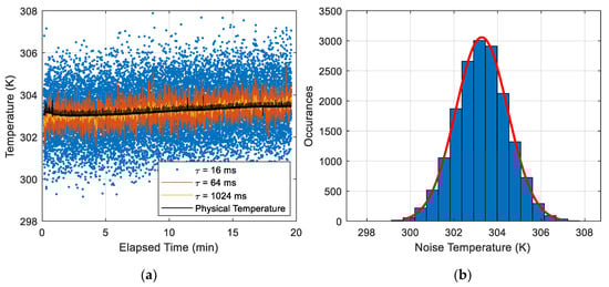
Figure 7.
Radiometer-measured noise temperatures during matched resistive source attached to the radiometer’s H port for quantifying PoLRa’s stability. (a) Noise temperature time series from different integration times are plotted along with the physical temperature of the source. (b) Histogram of raw ms samples shown in (a) and Gaussian fit of the distribution.
NEΔT can also be calculated theoretically by the equation [29]:
where is the system noise temperature discussed in Section 2.1 (627 K), is the RF bandwidth of the system, and is the post-detection integration time. The RF bandwidth is determined by the FE filters, which have a 3 dB passband of 27 MHz from 1400–1427 MHz. The theoretical NEΔT is provided, along with the experimental value, in Table 2. The theoretical values are likely slightly lower (~20%) because the radiometer was not perfectly stable in temperature during the experiment, and the bandwidth of the ideal rectangular filter assumed in Equation (11) overestimates the bandwidth of the real filter. The experimentally-determined NEΔT values do closely follow the trend of the respective theoretical values, suggesting that the radiometer is indeed measuring Gaussian thermal noise.
The difference between the mean noise temperature of the external resistive sources and their mean physical temperature was 0.02 K for the H polarization port, and 0.26 K for the V polarization port. The larger difference for the vertical polarization port could have been due to non-uniform heating of the cable or non-ideal thermal contact of the temperature sensor to the resistive source. The absolute accuracy specification of the thermocouple sensors is only 1 K. Considering this, measured noise temperatures of the external resistive source (attached to the H port) agree with its physical temperatures within the uncertainty of the sensors.
3.3. Uncertainty Characterization
With uncorrelated variables, the systematic uncertainty of calibrated noise temperature at the switch-port reference plane can be expressed using the variance formula as [30]:
where the prefix refers to the uncertainty associated with the proceeding variable. The systematic uncertainties , , of the measured voltages , , are <0.01 mV. When converted to temperature units by multiplication by the gain (~5 K/mV), these are much smaller than the uncertainties of measured physical temperatures , . Thus Equation (12) can be simplified to:
with:
and:
where the partial derivatives are calculated from the substitution of Equations (8) and (9) into (10). Given the specified temperature sensor uncertainty , and the ACS RMSE = 0.66 K from Section 3.1, the systematic uncertainty of PoLRa noise temperature measurements at the input ports can be calculated from Equation (13). We calculate for a range of , covering the range expected for measurements of terrestrial scenes. The total uncertainty of measured noise temperatures at the radiometer ports is then calculated as the root sum square of the systematic and statistical contributions:
The systematic uncertainty and total uncertainty are plotted for two different integration times in Figure 8. The uncertainty reaches a minimum when the measured noise temperature is roughly in-between the two calibration references (the RS and the ACS), and increases when the measured noise temperature requires extrapolation beyond the calibration reference points.
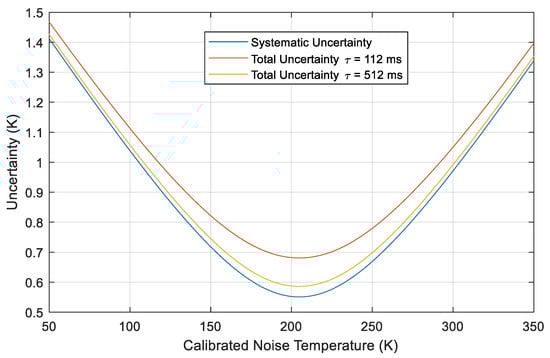
Figure 8.
Calculated systematic and total noise temperature uncertainty as a function of measured noise temperature for two different integration times .
Additional uncertainty sources, such as non-linearity, mismatch, and isolation [31], have been neglected in this analysis, as they are considered small compared to the uncertainty associated with the temperature sensors. Linearity estimates are provided with the detector, and mismatch between components and switch ports were all measured below −20 dB. The above uncertainty analysis has only considered internal uncertainty sources impacting the noise temperatures measured at the input ports of the switch.
When the antenna is viewing a natural footprint at the ground, additional uncertainty sources will arise, including potential radio-frequency interference (RFI). Though many modern radiometers have recently used high sample rate digital back ends for frequency-domain RFI mitigation, this approach still results in residual RFI, and is not foolproof [32]. Gaussian fitting of samples in the time domain is also an adequate means of RFI detection, as demonstrated in [28,33,34]. The Portable L-band Radiometer (PoLRa) discussed here uses the direct-detection architecture with total power detection for stability, simplicity, and low power consumption. Digital back ends of similar radiometers have been shown to consume at least 19 W [35], which is significantly more than the ~4 W used by PoLRa.
Conversion from antenna temperatures to footprint brightness temperatures used for retrieval of geophysical state parameters may also require a correction to consider the relatively large field-of-view of the antenna. When viewing the ground at non-nadir incidence angles, the linear polarizations at the antenna plane only correspond to the same linear polarizations at the boresight of the antenna. At off-nadir angles, the emissions from the ground must be corrected for polarization mixing; a detailed description of this procedure is provided in Appendix A of [20]. PoLRa-based retrievals of geophysical parameters, such as soil moisture, will be validated in the future using a network of in-situ soil moisture sensors.
4. Discussion
The design and characterization of the Portable L-band Radiometer (PoLRa) was outlined. Detailed technical discussion is presented to demonstrate that the radiometer hardware is functioning as expected, and to provide an estimate of its noise temperature measurement uncertainty.
While using a similar architecture common with other radiometers, PoLRa is unique in its antenna design, simple electronics, low power consumption, cost-effectiveness, and no required active temperature control. The radiometer presented here requires no temperature stability, due to the novel active cold source (ACS) characterization approach. Modeled cold-sky brightness temperature was used to characterize the response of ACS noise temperature to its varying physical temperature over the range of expected operational temperatures. This initial characterization allows full internal calibration of the radiometer afterwards, without need for further sky measurements.
The uncertainty of measured physical temperatures of the internal calibration noise sources (RS and ACS) are one of the primary contributors to the total uncertainty of noise temperatures measured at PoLRa’s input ports. The accuracy of the radiometer could likely be improved by improving the quality of the temperature sensor, but this would also necessitate investigation of second-order uncertainty terms, such as the non-linearity and mismatch. Total uncertainty values ranging between 0.6 K and 1.4 K, for the range of noise temperatures expected for measurements over natural footprints, is still low compared to satellite-based passive L-band measurements. For instance, SMOS has an uncertainty of 3 K or greater [36,37], and the NASA SMAP radiometer has a comparable uncertainty of 1.3 K [3].
The PolRa, with total mass less than 4 kg, including all mounting hardware, can be mounted on an unmanned aerial vehicle (UAV) such as a multi-copter drone, or can be used as a ground-based instrument on a tower or a simple pole. The radiometer could also be mounted on other vehicles, such as agricultural tractors, cars, or used on an aircraft. The low power consumption of the system allows operation with a compact battery, or with a small solar panel and battery system for off-grid ground-based use. The cost-effective design allows for production of a large number of such radiometers, which would allow for use in widespread networks valuable for satellite ground-validation purposes, or mass production of the hardware for use in agriculture and civil engineering.
Applications in agriculture could be for drone-based soil moisture and vegetation water content mapping. Soil moisture information could be used to inform smart irrigation systems, saving water, reducing crop stress, and increasing crop yield. Vegetation water content retrievals could be used for assessing crop health, and ripeness of crops, such as wheat and cereals, for optimal harvest timing.
Uses of the drone-based PoLRa in civil engineering would include finding leaks in levees and dams, and assessing soil moisture for surveys and building planning. Other potential uses of PoLRa in the future include landslide risk prediction and mitigation, and mitigating avalanche risk by spatial mapping of snow wetness and density.
This publication has introduced the hardware design, characterization, calibration, and uncertainty analysis of the PoLRa radiometer. We have only included free-space measurements of cold-sky for characterization of the active cold source (ACS) calibration reference. Other measurements introduced here have been performed in the laboratory. Future publications will introduce both ground- and drone-based measurements using the PoLRa, and associated retrievals of environmental parameters, including soil moisture and vegetation optical depth, for instance.
5. Conclusions
We have introduced a small, low-mass, and cost-effective L-band radiometer design, and provided characterization results to demonstrate its performance. L-band, with the lowest-frequency passive-protected band, from 1400–1427 MHz, provides penetration into natural media, such as soil and vegetation.
By mounting a portable low-mass radiometer on a multi-copter drone, pixel size of ~6 m or less is achievable. The PoLRa is also convenient as a ground-based radiometer for satellite validation networks, or any brightness temperature time-series measurement, and can be mounted on a simple automatic weather station type of infrastructure. This paper introduced the hardware design, calibration, characterization, and uncertainty analysis of the radiometer. The drone-based demonstration and results are reserved for a following publication.
We presented the block diagram of the direct-detect total power radiometer and the measured front-end filter response of the system. The radiometer is estimated to have a system noise temperature of K, based on the cascaded noise figure of the front-end and first LNA. The unique air-gapped patch antenna array design was shown, and the simulated and measured return loss and gain pattern presented. The antenna has a half-power full beamwidth of 37°, and is nearly symmetric with azimuth angle, resulting in a circular nadir-viewing pixel.
Section 3 presented the characterization of the active cold source (ACS) reference, the noise equivalent delta () temperature (), and the total radiometric uncertainty. The ACS was characterized along with the cable and antenna loss factor to a noise temperature root mean square error (RMSE) of 0.66 K. The experimentally determined for an integration time of s is 0.14 K, which is in close agreement with the theoretical value of 0.12 K, determined from the system noise temperature, integration time, and bandwidth. An integration time of 1 s actually takes about 4.4 s total, due to calibration views and views of the two polarizations. An integration time more realistic for future drone-based operation is about 100 ms, corresponding to a total measurement time of 480 ms and of 0.4 K.
The total uncertainty of the radiometer is the combination of systematic and statistical uncertainty contributions. The systematic uncertainty is determined from propagation of the calibration reference uncertainties, whereas the statistical uncertainty is equivalent to the , and is a function of the integration time. The total uncertainty is found to range between 0.6 K and 1.4 K over a range of expected natural brightness temperatures from 50 K to 350 K. This value is less than the radiometric uncertainty of the ESA SMOS satellite, and comparable to that of NASA’s SMAP instrument.
6. Patents
A European Patent Office application was the result of the antenna and electronics design of the radiometer discussed in this paper. The patent is filed in the name of the Swiss Federal Research Institute WSL, with Dr. Derek Houtz as the inventor.
Author Contributions
Conceptualization: D.H.; methodology: D.H., M.S., and R.N.; software: D.H.; validation: D.H., M.S., and R.N.; formal analysis: D.H.; investigation: D.H., M.S., and R.N.; resources: D.H., M.S., and R.N.; data curation: D.H.; writing—original draft preparation: D.H.; writing—review and editing: R.N. and M.S.; visualization: D.H.; supervision: M.S.; project administration: M.S.; funding acquisition: D.H. All authors have read and agreed to the published version of the manuscript.
Funding
This research received no external funding.
Conflicts of Interest
The authors declare no conflict of interest.
References
- Kerr, Y.H.; Waldteufel, P.; Wigneron, J.P.; Martinuzzi, J.M.; Font, J.; Berger, M. Soil moisture retrieval from space: The Soil Moisture and Ocean Salinity (SMOS) mission. IEEE Trans. Geosci. Remote Sens. 2001, 39, 1729–1735. [Google Scholar] [CrossRef]
- Le Vine, D.M.; Lagerloef, G.S.; Colomb, F.R.; Yueh, S.H.; Pellerano, F.A. Aquarius: An instrument to monitor sea surface salinity from space. IEEE Trans. Geosci. Remote Sens. 2007, 45, 2040–2050. [Google Scholar] [CrossRef]
- Entekhabi, D.; Njoku, E.G.; O’Neill, P.E.; Kellogg, K.H.; Crow, W.T.; Edelstein, W.N.; Entin, J.K.; Goodman, S.D.; Jackson, T.J.; Johnson, J.; et al. The Soil Moisture Active Passive (SMAP) Mission. Proc. IEEE. 2010, 98, 704–716. [Google Scholar] [CrossRef]
- Kerr, Y.H.; Waldteufel, P.; Richaume, P.; Wigneron, J.P.; Ferrazzoli, P.; Mahmoodi, A.; Al Bitar, A.; Cabot, F.; Gruhier, C.; Juglea, S.E.; et al. The SMOS Soil Moisture Retrieval Algorithm. IEEE Trans. Geosci. Remote Sens. 2012, 50, 1384–1403. [Google Scholar] [CrossRef]
- Schwank, M.; Naderpour, R.; Mätzler, C. “Tau-Omega”- and Two-Stream Emission Models Used for Passive L-Band Retrievals: Application to Close-Range Measurements over a Forest. Remote Sens. 2018, 10, 1868. [Google Scholar] [CrossRef]
- Font, J.; Camps, A.; Borges, A.; Martín-Neira, M.; Boutin, J.; Reul, N.; Kerr, Y.H.; Hahne, A.; Mecklenburg, S. SMOS: The challenging sea surface salinity measurement from space. Proc. IEEE 2010, 98, 649–665. [Google Scholar] [CrossRef]
- Rodríguez-Fernández, N.J.; Mialon, A.; Mermoz, S.; Bouvet, A.; Richaume, P.; Al Bitar, A.; Al-Yaari, A.; Brandt, M.; Kaminski, T.; Le Toan, T. An evaluation of SMOS L-band vegetation optical depth (L-VOD) data sets: High sensitivity of L-VOD to above-ground biomass in Africa. Biogeosciences 2018, 15, 4627–4645. [Google Scholar] [CrossRef]
- Li, X.; Al-Yaari, A.; Schwank, M.; Fan, L.; Frappart, F.; Swenson, J.; Wigneron, J.-P. Compared performances of SMOS-IC soil moisture and vegetation optical depth retrievals based on Tau-Omega and Two-Stream microwave emission models. Remote Sens. Environ. 2020, 236, 111502. [Google Scholar] [CrossRef]
- Naderpour, R.; Schwank, M. Snow Wetness Retrieved from L-Band Radiometry. Remote Sens. 2018, 10, 359. [Google Scholar] [CrossRef]
- Schwank, M.; Naderpour, R. Snow Density and Ground Permittivity Retrieved from L-Band Radiometry: Melting Effects. Remote Sens. 2018, 10, 354. [Google Scholar] [CrossRef]
- Houtz, D.; Naderpour, R.; Schwank, M.; Steffen, K. Snow wetness and density retrieved from L-band satellite radiometer observations over a site in the West Greenland ablation zone. Remote Sens. Environ. 2019, 235, 111361. [Google Scholar] [CrossRef]
- Schwank, M.; Matzler, C.; Wiesmann, A.; Wegmuller, U.; Pulliainen, J.; Lemmetyinen, J.; Rautiainen, K.; Derksen, C.; Toose, P.; Drusch, M. Snow Density and Ground Permittivity Retrieved from L-Band Radiometry: A Synthetic Analysis. IEEE J. Sel. Top. Appl. Earth Obs. Remote Sens. 2015, 8, 3833–3845. [Google Scholar] [CrossRef]
- Rautiainen, K.; Parkkinen, T.; Lemmetyinen, J.; Schwank, M.; Wiesmann, A.; Ikonen, J.; Derksen, C.; Davydov, S.; Davydova, A.; Boike, J. SMOS prototype algorithm for detecting autumn soil freezing. Remote Sens. Environ. 2016, 180, 346–360. [Google Scholar] [CrossRef]
- Rautiainen, K.; Lemmetyinen, J.; Schwank, M.; Kontu, A.; Menard, C.B.; Matzler, C.; Drusch, M.; Wiesmann, A.; Ikonen, J.; Pulliainen, J. Detection of soil freezing from L-band passive microwave observations. Remote Sens. Environ. 2014, 147, 206–218. [Google Scholar] [CrossRef]
- Kaleschke, L.; Tian-Kunze, X.; Maass, N.; Makynen, M.; Drusch, M. Sea ice thickness retrieval from SMOS brightness temperatures during the Arctic freeze-up period. Geophys. Res. Lett. 2012, 39. [Google Scholar] [CrossRef]
- Acevo-Herrera, R.; Aguasca, A.; Bosch-Lluis, X.; Camps, A.; Martínez-Fernández, J.; Sánchez-Martín, N.; Pérez-Gutiérrez, C. Design and first results of an UAV-borne L-band radiometer for multiple monitoring purposes. Remote Sens. 2010, 2, 1662–1679. [Google Scholar] [CrossRef]
- McIntyre, E.M.; Gasiewski, A.J. An ultra-lightweight L-band digital Lobe-Differencing Correlation Radiometer (LDCR) for airborne UAV SSS mapping. In Proceedings of the 2007 IEEE International Geoscience and Remote Sensing Symposium, Barcelona, Spain, 23 July 2007; pp. 1095–1097. [Google Scholar]
- Davenport, I.J.; Fernández-Gálvez, J.; Gurney, R.J. A sensitivity analysis of soil moisture retrieval from the tau-omega microwave emission model. IEEE Trans. Geosci. Remote Sens. 2005, 43, 1304–1316. [Google Scholar] [CrossRef]
- Mo, T.; Choudhury, B.J.; Schmugge, T.J.; Wang, J.R.; Jackson, T.J. A Model for Microwave Emission from Vegetation-Covered Fields. J. Geophys. Res. Ocean. Atmos. 1982, 87, 1229–1237. [Google Scholar] [CrossRef]
- Naderpour, R.; Houtz, D.; Schwank, M. Snow Wetness Retrieved from Close-Range L-band Radiometry in the Western Greenland Ablation Zone. J. Glaciol. 2020, in press. [Google Scholar]
- De Roo, R.D.; Ruf, C.S.; Sabet, K. An L-band radio frequency interference (RFI) detection and mitigation testbed for microwave radiometry. In Proceedings of the 2007 IEEE International Geoscience and Remote Sensing Symposium, Barcelona, Spain, 23 July 2007; pp. 2718–2721. [Google Scholar]
- Application Notes. 57-1: Fundamentals of RF and Microwave Noise Figure Measurements. 2000. Available online: https://www.keysight.com/ch/de/assets/7018-06808/application-notes/5952-8255.pdf (accessed on 24 July 2020).
- Schwank, M.; Wiesmann, A.; Werner, C.; Matzler, C.; Weber, D.; Murk, A.; Volksch, I.; Wegmuller, U. ELBARA II, an L-band radiometer system for soil moisture research. Sensors 2010, 10, 584–612. [Google Scholar] [CrossRef]
- Pellarin, T.; Wigneron, J.P.; Calvet, J.C.; Berger, M.; Douville, H.; Ferrazzoli, P.; Kerr, Y.H.; Lopez-Baeza, E.; Pulliainen, J.; Simmonds, L.P.; et al. Two-year global simulation of L-band brightness temperatures over land. IEEE Trans. Geosci. Remote Sens. 2003, 41, 2135–2139. [Google Scholar] [CrossRef]
- Le Vine, D.M.; Abraham, S. Galactic noise and passive microwave remote sensing from space at L-band. IEEE Trans. Geosci. Remote Sens. 2004, 42, 119–129. [Google Scholar] [CrossRef]
- Sobjaerg, S.S.; Skou, N.; Balling, J.E. Measurements on active cold loads for radiometer calibration. IEEE Trans. Geosci. Remote Sens. 2009, 47, 3134–3139. [Google Scholar] [CrossRef]
- de la Jarrige, E.L.; Escotte, L.; Goutoule, J.; Gonneau, E.; Rayssac, J. SiGe HBT-based active cold load for radiometer calibration. IEEE Microw. Wirel. Compon. Lett. 2010, 20, 238–240. [Google Scholar] [CrossRef]
- Naderpour, R.; Schwank, M.; Matzler, C. Davos-Laret Remote Sensing Field Laboratory: 2016/2017 Winter Season L-Band Measurements Data-Processing and Analysis. Remote Sens. 2017, 9, 1185. [Google Scholar] [CrossRef]
- Racette, P.; Lang, R.H. Radiometer design analysis based upon measurement uncertainty. Radio Sci. 2005, 40, 1–22. [Google Scholar] [CrossRef]
- Ku, H.H. Notes on the use of propagation of error formulas. J. Res. Natl. Bur. Stand. 1966, 70, 263–273. [Google Scholar] [CrossRef]
- Randa, J.P. Uncertainties in NIST Noise-Temperature Measurements. In Technical Note (NIST TN)-1502; 1998. Available online: https://www.nist.gov/publications/uncertainties-nist-noise-temperature-measurements (accessed on 24 July 2020).
- Majurec, N.; Park, J.; Niamsuwan, N.; Frankford, M.; Johnson, J.T. Airborne L-band RFI observations in the smapvex08 campaign with the L-band interference suppressing radiometer. In Proceedings of the 2009 IEEE International Geoscience and Remote Sensing Symposium, Cape Town, South Africa, 12 July 2009; pp. 158–161. [Google Scholar]
- Guner, B.; Johnson, J.T.; Niamsuwan, N. Time and frequency blanking for radio-frequency interference mitigation in microwave radiometry. IEEE Trans. Geosci. Remote Sens. 2007, 45, 3672–3679. [Google Scholar] [CrossRef]
- Tarongi, J.M.; Camps, A. Normality analysis for RFI detection in microwave radiometry. Remote Sens. 2010, 2, 191–210. [Google Scholar] [CrossRef]
- Lahtinen, J.; Ruokokoski, T.; Kristensen, S.S.; Skou, N. Intelligent Digital Back-End for Real-Time RFI Detection and Mitigation in Microwave Radiometry. 2011. Available online: https://www.researchgate.net/publication/268063678_Intelligent_Digital_Back-End_for_Real-Time_RFI_Detection_and_Mitigation_in_Microwave_Radiometry (accessed on 24 July 2020).
- Munoz-Sabater, J.; de Rosnay, P.; Jimenez, C.; Isaksen, L.; Albergel, C. SMOS brightness temperature angular noise: Characterization, filtering, and validation. IEEE Trans. Geosci. Remote Sens. 2013, 52, 5827–5839. [Google Scholar] [CrossRef]
- McMullan, K.; Brown, M.A.; Martín-Neira, M.; Rits, W.; Ekholm, S.; Marti, J.; Lemanczyk, J. SMOS: The payload. IEEE Trans. Geosci. Remote Sens. 2008, 46, 594–605. [Google Scholar] [CrossRef]
© 2020 by the authors. Licensee MDPI, Basel, Switzerland. This article is an open access article distributed under the terms and conditions of the Creative Commons Attribution (CC BY) license (http://creativecommons.org/licenses/by/4.0/).