Microphysical and Polarimetric Radar Signatures of an Epic Flood Event in Southern China

Abstract

An extremely heavy rainfall event hit Guangdong province, China, from 27 August to 1 September 2018. There were two different extreme rain regions, respectively, at the Pearl River estuary and eastern Guangdong, and a record-breaking daily precipitation of 1056.7 mm was observed at Gaotan station on 30 August. This paper utilizes a suite of observations from soundings, a gauge network, disdrometers, and polarimetric radars to gain insights to the two rainfall centers. The large-scale meteorological forcing, rainfall patterns, and microphysical processes, as well as radar-based precipitation signatures are investigated. It is concluded that a west-moving monsoon depression played a critical role in sustaining the moisture supply to the two extreme rain regions, and the combined orographic enhancement further contributed to the torrential rainfall over Gaotan station. The raindrop size distributions (DSD) observed at Zhuhai and Huidong stations, as well as the observed polarimetric radar signatures indicate that the rainfall at Doumen region was characterized by larger raindrops but a lower number concentration compared with that at Gaotan region. In addition, the dual-polarization radars are used to quantify precipitation intensity during this extreme event, providing timely information for flood warning and emergency management decision-making.

1. Introduction

Torrential rainfall events are one of the most severe disasters around the world [1,2]. The extreme rainfall and induced floods, landslides, debris flows gravely threaten life and property. The precipitation microphysics such as raindrop size distribution (DSD) serves as a fundamental bridge in deriving radar quantitative precipitation estimation (QPE) algorithms, which is critical for improving the accuracy of precipitation estimation and predictions [3,4]. Accurate precipitation estimates are also important input to the flash flood guidance systems for flood forecast, as well as subsequent warning operations and emergency management decision-making [5]. Therefore, a better understanding of precipitation microphysics and accurate quantitative precipitation estimation for extreme rain are important for flood warning and emergency management decision-making.

Under the influence of the East Asian monsoon, the Indian monsoon, the western Pacific subtropical high, as well as Tibetan Plateau, southern China is severely affected by heavy rain events during warm seasons (May to September), which usually cause floods and landslides [6,7,8]. From 27 August to 1 September 2018, an extremely heavy rainfall occurred over Guangdong province, especially in the south and east parts of Guangdong. There were two different extreme rainfall centers on 29 August and 30 August, respectively: one was located around Doumen station in Zhuhai, and the other was located at Gaotan station in Huidong. A record-breaking daily precipitation of 1056.7 mm was observed at Gaotan station on 30 August. This heavy rainfall caused catastrophic floods in many cities such as Huizhou, Shantou, Zhuhai, affecting more than 1 million people, causing directed financial losses around USD 144 million (https://www.thepaper.cn/newsDetail_forward_2404157). Moreover, a recent study has shown that extreme precipitation shows an increasing trend in south China during the last several decades [9], which highlights the importance of accurate precipitation measurement and modeling.

However, it is always a challenge to obtain accurate precipitation estimation. Gauges, weather radars, and satellite-based sensors are three main methods to measure precipitation [10]. Gauges can provide the most direct and precise precipitation observations. However, they are limited to fixed locations, and the networks of gauges are sparse. Therefore, interpolation is required to produce areal rainfall mapping and the interpolation method could lead to significant errors [11]. Satellite rainfall data has the advantage of large-scale spatial coverage, so the derived spatial distribution of rainfall is more complete. However, the satellite data also suffers from various sources of errors, including systematic error, random error, etc. Additionally, the spatial and temporal resolutions are very low, which has posed great difficulty in capturing the structure and evolution of small scale but strong storms [12]. In such cases, the only practical way to achieve a comprehensive estimation of precipitation is weather radar, which can provide real-time high-resolution monitoring over large areas [13,14].

Eight weather radars in the Guangdong area have completed dual-polarization upgrades in 2017 to improve disaster warning and forecasting capabilities. Compared to traditional single-polarization radar, the dual-polarization radar can measure polarimetric parameters including differential reflectivity $Z_{dr}$, differential phase shift ${\varphi }_{dp}$, and co-polar correlation coefficient ${\rho }_{HV}$[14]. These parameters can be used to reveal microphysical properties of different hydrometeors [15,16,17,18] and improve quantitative precipitation estimation [14,19]. Meanwhile, several disdrometers have been installed in Guangdong province. Though they provide point measurements, the accumulation of time decreases the spatial variability of local precipitation microphysics [20]. Therefore, these disdrometers can provide detailed knowledge of local DSD information, which is critical in understanding the microphysical characteristics of precipitation and improving microphysical parameterization schemes in the numerical weather prediction models [4,21].

The primary purpose of this study is to conduct a comprehensive analysis of this extreme event from 27 August to 1 September 2018, based on various in situ and remote sensing observations including rain gauges, polarimetric radars, disdrometers, and reanalysis data so as to gain a better understanding of the epic flood events as such, especially to explore the potential of polarimetric radars to resolve the microphysics and quantify the precipitation. This study is also part of our effort in improving precipitation monitoring, forecast, and associated hydrologic responses in southern China. The paper is organized as follows. The study domain and dataset are described in Section 2. The synoptic environment of this extreme rainfall event is detailed in Section 3. The rainfall pattern and microstructural characteristics of this rainstorm observed by gauge and disdrometers, as well as the associated polarimetric radar signatures are detailed in Section 4. Section 5 summarizes the main findings of this study and suggests future directions of this research.

2. Data and Methodology

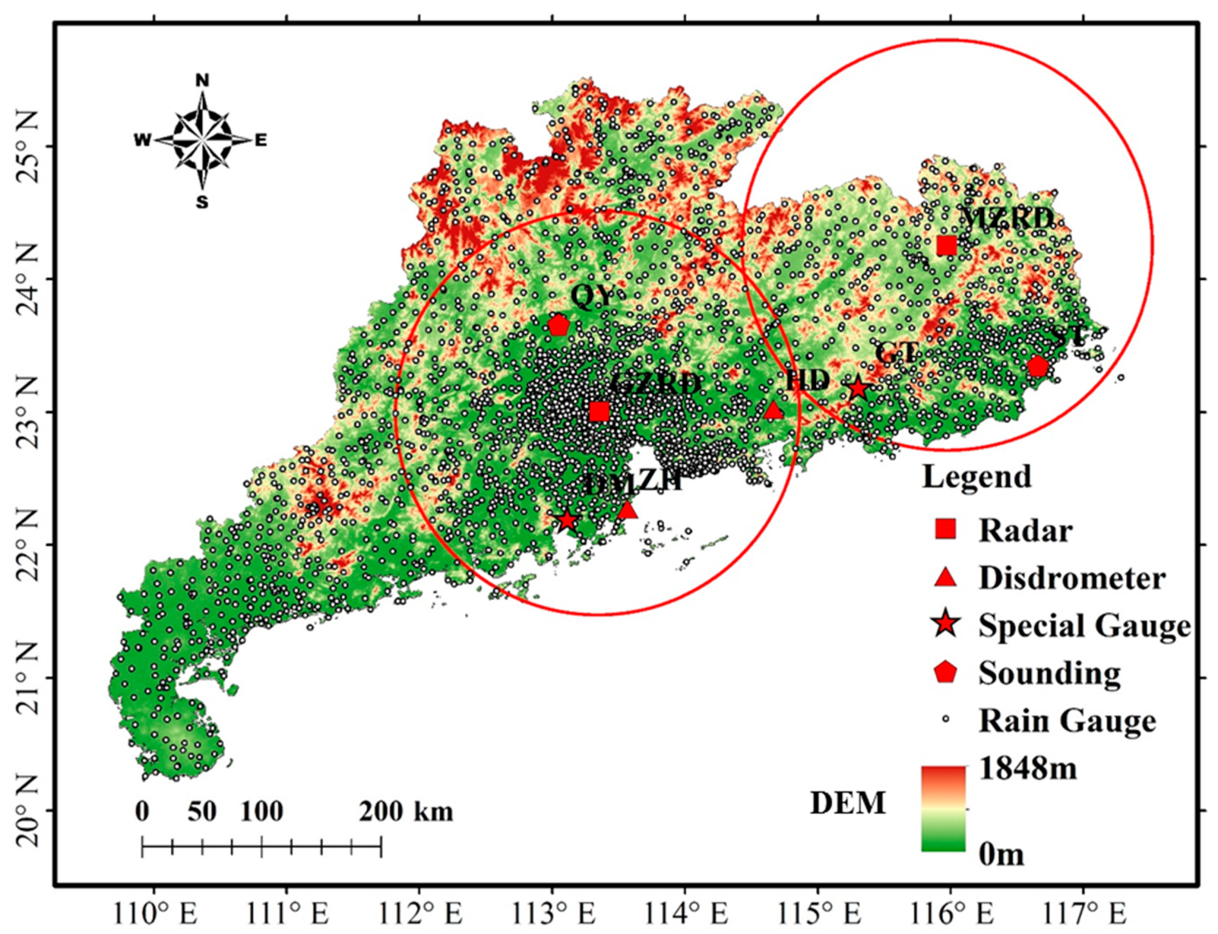
2.1. Data

The observational data used in this study include rainfall measurements from a dense gauge network, two S-band polarimetric radars, and two second-generation Particle Size and Velocity (Parsivel²) disdrometers in Guangdong. The instrument locations and the two special gauge stations (Gaotan and Doumen) are shown in Figure 1. The National Centers for Environmental Prediction (NCEP) final operational model global analysis data (NCEP-FNL) available every 6 h with a resolution of 0.25° × 0.25° at 31 vertical levels (http://rda.ucar.edu/datasets/ds083.2//#!access) are used to resolve the synoptic condition [22], along with the sounding data collected at 00:00 and 12:00 UTC at Qingyuan (QY) and Shantou (ST) (No. 59280, and No. 59316 from the University of Wyoming: http://weather.uwyo.edu/upperair/sounding.html).

2.2. Raindrop Size Distribution

In order to understand the microphysics of the extreme rain, two disdrometers nearest to Doumen and Gaotan gauge stations are used to provide the DSD observation. These two disdrometers are located at Zhuhai and Huidong, collocated with rain gauges within 20 m. Both disdrometers are optical disdrometers with a 54 cm² horizontal sample area and are configured with 1-min sampling resolution to measure the DSD and fall velocity of raindrops [23,24]. The disdrometer performance has been assessed and improved since it was invented, and many previous studies have been conducted with this device [25,26,27,28]. In particular, the velocity and particle sizes are divided into 32 non-uniform bins, varying from 0.05 to 20.8 m s⁻¹ for bin-center velocity and 0.062–24.5 mm for bin-center diameter (for detailed information in the user manual, https://www.manualslib.com/products/Ott-Parsivel2-5889584.html). The direct measurements from disdrometer are the number of raindrops at each velocity (i) and diameter (j) bin. Here, we take the bin-center value of each bin as the corresponding value. Several parameters used to describe the characteristics of DSD are calculated in the following.

The total number of raindrops can be calculated as follows:

$$Td={\sum }_{i=1}^{32}{\sum }_{j=1}^{32}{n}_{i,j},$$

(1)

where $n_{i,j}$ is the number of drops at each bin.

The number concentration of raindrops per unit volume for the $j$th diameter bin $N(D_j)$ can be calculated as follows:

$$N(D_j)={\sum }_{i=1}^{32}\frac{n_{i,j}}{A·\Delta t·V_i·\Delta D_j},$$

(2)

where $N(D_j)$ is in m⁻³ mm⁻¹; $A$ is the sampling area in m²; $\Delta t$ is the sampling time interval in s; $A$ and $\Delta t$ are, respectively, 0.0054 m² and 60 s in this study; $\Delta D_j$ (mm) is the diameter interval from $D_j$ to $D_{j+1}$ for the jth diameter bin; $V_i$ (m s⁻¹) is the fall speed for the $i$th velocity class. Due to the measurement error, especially for larger size drops [23], the empirical terminal velocity–diameter ($V – D$) relation in Atlas et al. [29] is adopted in this study:

$$V(D_j)=9.65-10.3\exp (-0.6D_j),$$

(3)

The drops with velocity out the range of ±60% $V(D_j)$are removed from the analysis [30].

The total number concentration $N_t$ (m⁻³), the mass weighted diameter $D_m$ (mm), and normalized intercept parameter $N_w$ (m⁻³ mm⁻¹) [14] are derived as:

$$N_t={\sum }_{i=i}^{32}{\sum }_{j=1}^{32}\frac{n_{i,j}}{A·\Delta t·V_i},$$

(4)

$$D_m=\frac{{\sum }_{j=1}^{32}N(D_j)·D_j^4·\Delta D_j}{{\sum }_{j=1}^{32}N(D_j)·D_j^3·\Delta D_j},$$

(5)

$$N_w=\frac{4^4}{\pi {\rho }_w}\left(\frac{{10}^{3}W}{D_m^4}\right),$$

(6)

$D_m$ is closely related to the drop size; $N_t$and $N_w$ are related to the number of raindrops. All these parameters are important in representing the DSD characteristics.

The integral rainfall parameters including rain rate $R$ (mm h⁻¹) and liquid water content $W$ (g m⁻³) are calculated based on the following equations:

$$R= \frac{6\mathsf{\pi }}{{10}^4{\rho }_w}{\sum }_{j=1}^{32}V(D_j){D_j}^{3}N(D_j)\Delta D_j,$$

(7)

$$W=\frac{\pi {\rho }_w}{6\times {10}^3}{\sum }_{j=1}^{32}{D_j}^{3}N(D_j)\Delta D_j,$$

(8)

where ${\rho }_w$ is the water density (1.0 g cm⁻³).

Meanwhile, a series of polarimetric radar variables are simulated at S-band frequency based on the DSD measurements using the T-matrix method [31,32,33], including horizontal reflectivity ${\mathrm{Z}}_h$ (mm⁶ m⁻³, or ${\mathrm{Z}}_H$ in dBZ), differential reflectivity ${\mathrm{Z}}_{dr}$ (dB), and specific differential phase $K_{dp}$(degree km⁻¹). The drop shape model used in the simulation is the one proposed by Thurai et al. [34] and temperature is 20 $℃$. The canting angle is not taken into account (i.e., canting angle is 0) as the DSD measurements are near ground.

We also want to note that to minimize the measurement errors and improve data reliability, several quality control procedures were applied on the 1-min DSD data. First, because of the low signal-to-noise ratios, the first two diameter bins are always empty, so the data in first two bins are eliminated in the analysis [23]. Second, the 1-min sample data with total raindrop number smaller than 10 or the derived rain rate less than 0.1 mm h⁻¹ are considered noise and removed [23]. Then, if the continuous data satisfying the above conditions last less than 5 min, they will be ignored to avoid the spurious and erratic measurements [25,35]. Additionally, threshold on simulated radar parameter (i.e., ${\mathrm{Z}}_H <$ 55 dBZ) is used to further guarantee the creditability of the measured DSD data. The DSDs with the radar parameters out of the range are deleted to avoid mixed phase hydrometeors.

2.3. Radar Quantitative Precipitation Estimation

The two S-band radars are located at Guangzhou (hereafter referred as GZRD, 23.004° N, 113.355° E, 179 m) and Meizhou (MZRD, 24.256° N, 115.975° E, 423 m). Both radars are configured with a 6-min time resolution and 250-m range gate spacing, and have undergone rigorous quality control to ensure the data quality [36]. These two radars are used to monitor the evolution of the storm system and associated microphysical signatures. Moreover, these two radars are applied to estimate the rainfall to show the great potential of radar quantitative precipitation estimation.

For polarimetric radar, $R(Z_H)$, $R(K_{dp})$, $R(Z_H,Z_{dr})$, $R(Z_{dr},K_{dp})$ are the four relations commonly used to estimate rainfall [14]. The parameters (i.e., coefficients and exponents) in these relations are determined by the local precipitation microphysics, and are usually derived from the in situ DSD data. The representative of these parameters and how to combine different relations are the key issue in deriving radar QPE [14].

In this study, four rainfall algorithms are applied to quantify the precipitation intensity and amounts during this event. These algorithms belong to two categories: one is $R(Z_H)$ relation, i.e., WRS-88D Z-R relationship [13] and localized Z-R relationship; another is a combination of the four rainfall relations (i.e., $R(Z_H)$, $R(K_{dp})$, $R(Z_H,Z_{dr})$, $R(Z_{dr},K_{dp})$), i.e., the “adapted algorithm” described by Xia et al. [36] and the localized blended relation. Both Z-R relations are commonly used for single-polarized radar. The “adapted algorithm” is derived from DSD data and adjusted based on gauge observation and it has been demonstrated during several typhoon events in Southern China, which showed great performance [36].

Based on the nonlinear least-square method with the DSD data from two stations, the localized relations are fitted as follows:

$$R(Z_H) = 0.06082 \times {10}^{0.05709Z_H},$$

(9)

$$R(K_{dp}) = 40.4615K_{dp}^{0.7703}$$

(10)

$$R(Z_H,Z_{dr}) = 0.00632 \times {10}^{0.09134Z_H}{10}^{-0.3325Z_{dr}}$$

(11)

$$R(Z_{dr},K_{dp}) = 84.4318K_{DP}^{0.9377}{10}^{-0.1588Z_{dr}}$$

(12)

where Equation (9) is referred to as the localized Z-R relation, and the localized blended relation is a combination of Equations (10)–(12), using the same logic described by Xia et al. [36].

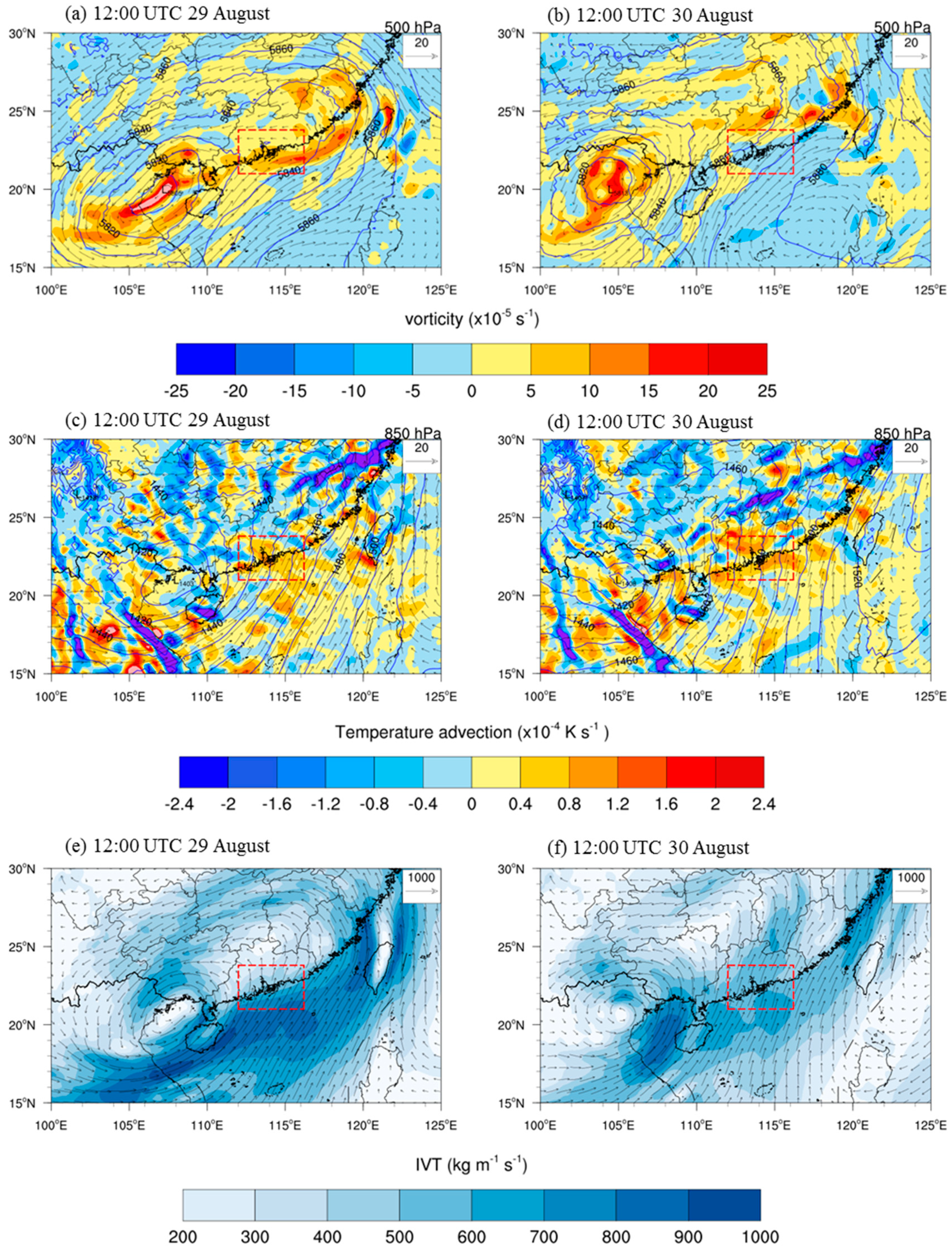
3. Synoptic Environment during This Epic Rainfall Event

From 27 to 31 August 2018, a monsoon depression evolved, moving west from the East China Sea. The resultant precipitation system was moving from west to east along the coast, causing heavy precipitation nearly over the whole Guangdong province, especially in the south and southeast parts of Guangdong on 29 and 30 August. The synoptic evolution of this precipitation system was analyzed using the NCEP-FNL data at 12:00 UTC 29 August and 12:00 UTC 30 August (Figure 2). Additionally, Figure 3 shows the stratification curve and convective available potential energy (CAPE) based on the sounding data at QY and ST stations.

It can be seen that the entire region of southern China was under the influence of a monsoon depression across the mid- and lower-troposphere on 29 August. The depression moved west, bringing strong moistures transported to Guangdong province driven by the persistent south and southwest wind (Figure 2a,b). In the coastal areas of Guangdong, warm advection from the ground and lower troposphere continued to transport warm air to inland areas (Figure 2c,d). Due to the combined evolution of depression and topography lifting effect, the precipitation system was further strengthened on 30 August. The wind and temperature changes between Guangdong and the adjacent South China Sea were more violent (Figure 2c,d). Meanwhile, the vertically integrated vapor transport (IVT) over the coastal zone was much stronger on 30 August than that on 29 August (Figure 2e,f).

Figure 3a illustrates the sounding curves at 12:00 UTC 29 August at QY station. The large convective available potential energy (CAPE, ≈860 J kg⁻¹) and low level of free convection (LFC, ≈980 hPa) suggested that the atmospheric environment was favorable for the development of convection [37]. At 20:00 UTC 30 August, the CAPE became larger and LFC became lower, indicating that the convection had further developed. The soundings at ST station also showed a conducive environment for convection development though the CAPE decreased slightly from the 29th to 30th.

4. Precipitation Analysis Results and Discussion

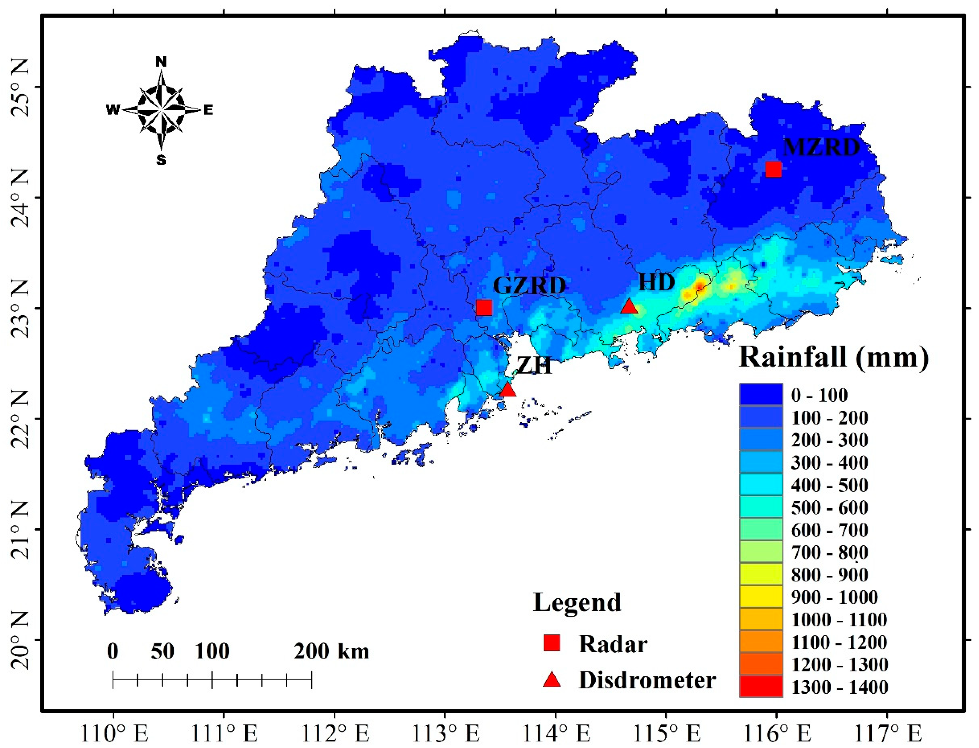
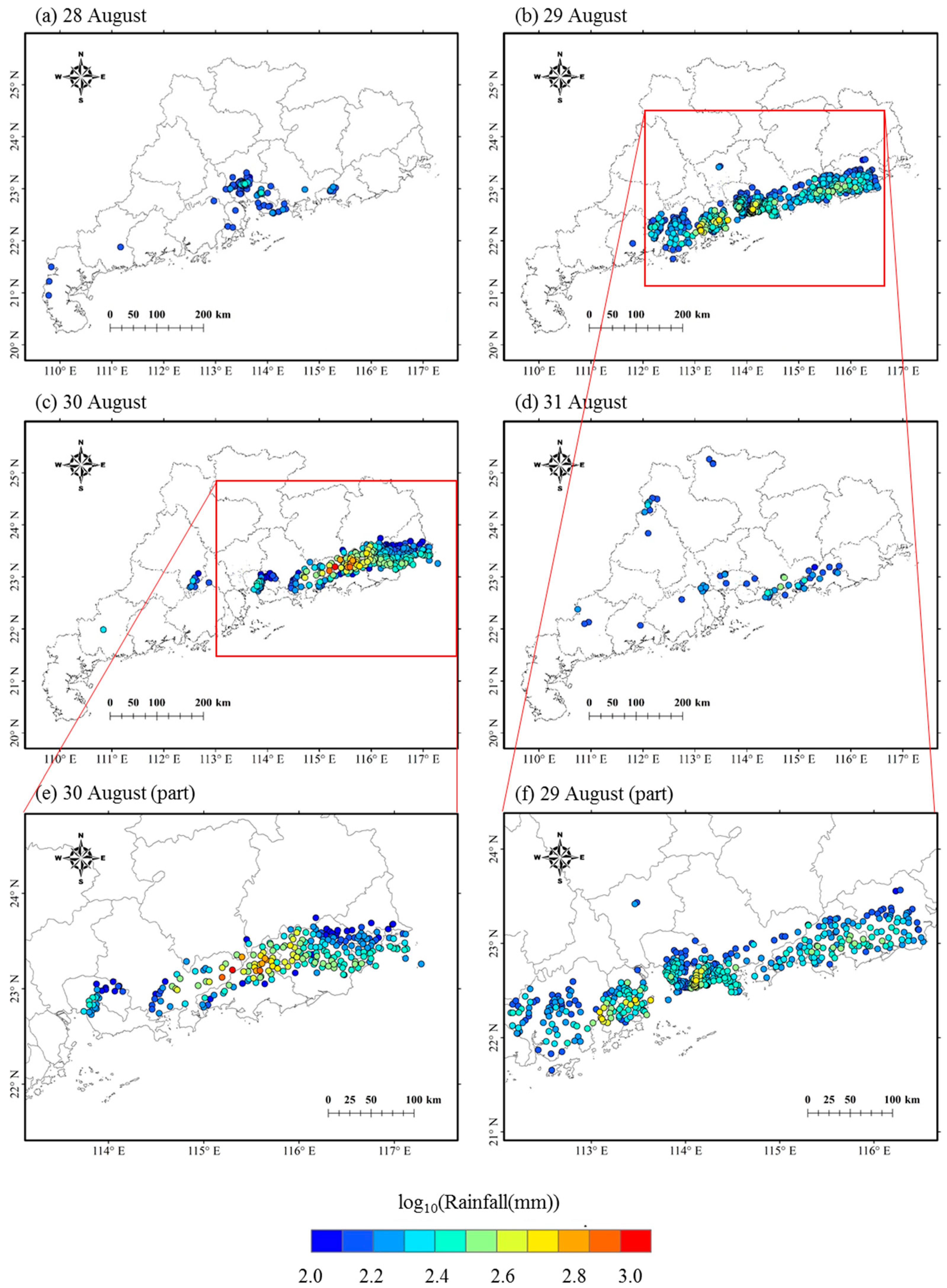
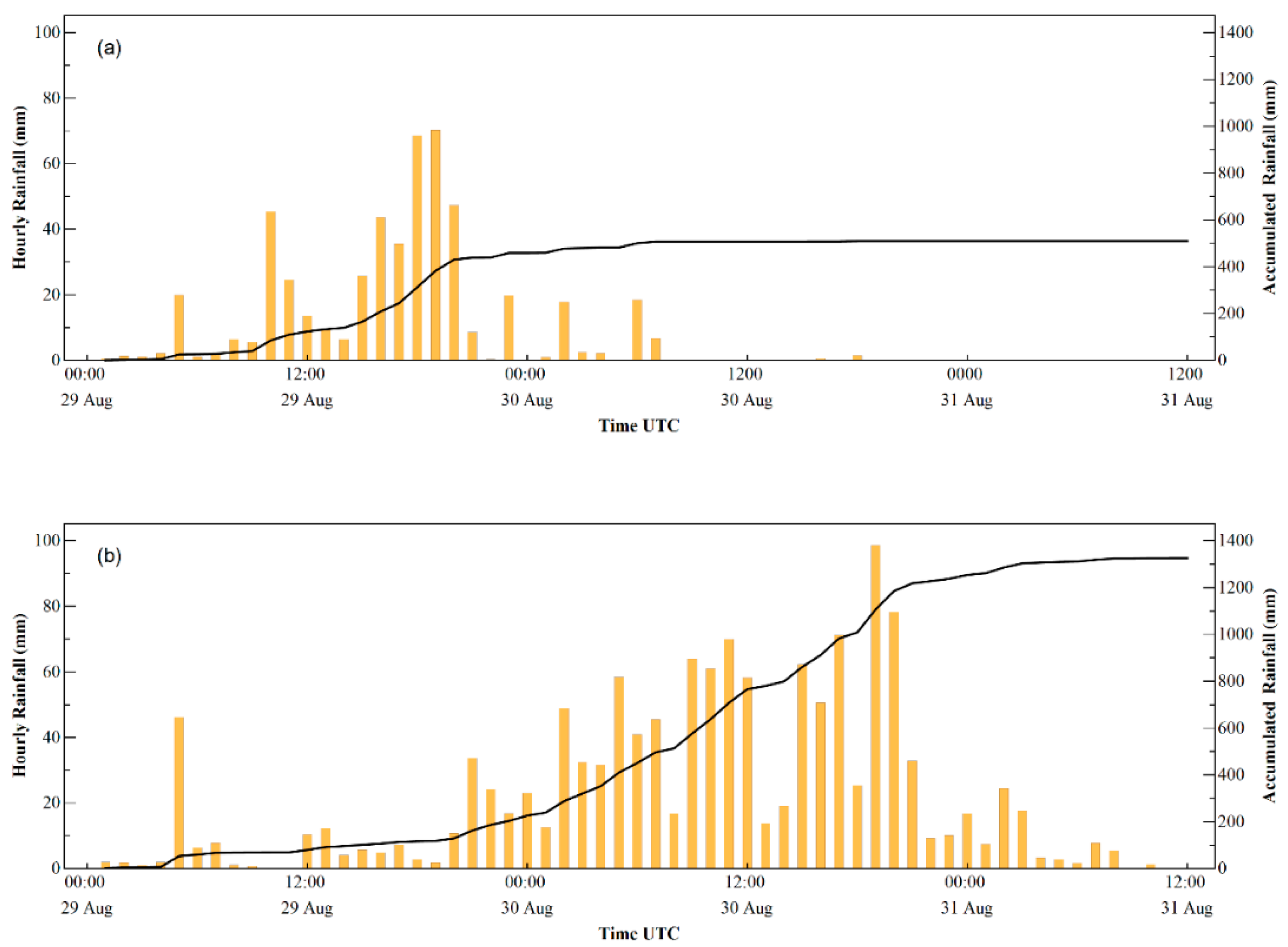
4.1. Precipitation Pattern Observed by a Gauge Network

Figure 4 shows the spatial distribution of the cumulative rainfall in Guangdong during the period from 00:00 UTC 27 August to 00:00 UTC 2 September based on the gauge hourly precipitation data using Inverse Distance Weighted (IDW) interpolation method. This result was only used for visualization so as to get a general sense of the geographic distribution of rainfall. Obviously, this rainstorm affected most regions of Guangdong, with the extreme rainfall occurring at the southeast part and gradually decreased to the northwest of Guangdong. The gauge maximum cumulative rainfall was 1394.6 mm recorded at Gaotan station (23.1883 °N, 115.3044 °E), which set a new record of cumulative rainfall during a single event in Guangdong. Meanwhile, the maximum daily rainfall of 1056.7mm was also recorded at Gaotan station from 21:00 UTC 29 August to 21:00 UTC 30 August, which broke the historical daily rainfall record of 924.3 mm on 17 August 2013 [7].

Figure 5 shows the distribution of the daily rainfall that exceeded 100 mm from 28 to 31 August. It is clear that the rainfall is mainly concentrated on 29 and 30 August. There is a clear rain band along the coast on 29 August, with a gradient of accumulated rainfall decreasing from the coast towards the inland region, which can be partially attributed to the land-sea roughness contrasts [38]. On 30 August, the rain band moved a little towards northeast and inland region, with extremely high accumulated value (1041.1 mm) concentrated at Gaotan station, which could be due to the combined effect of terrain and evolved synoptic condition. To further reveal the two rainfall processes, Figure 6 shows the time series of rainfall collected at two gauges where extreme daily rainfall concentrated on these two days. One station is located at Doumen (22.1967 °N, 1153.1131 °E) in Zhuhai, representing the rainfall on 29 August, when the daily rainfall reached 458.6 mm. Another station is Gaotan station, representing the most extreme rainfall pattern both for 30 August and the whole event.

The differences between the two stations are clear: Doumen station experienced heavy rainfall mainly on 29 August, while Gaotan station experienced a heavier and longer rainfall from late 29 August to early 31 August. Doumen station experienced three major rainfall stages on 29 August: first from 00:00 to 06:00 UTC, second from 06:00 to 14:00 UTC, and third from 14:00 to 23:00 UTC. The third stage was longer and stronger than the first two stages, with a maximum hourly rainfall of 70.2 mm from 1800 to 1900 UTC 29 August. After 0800 UTC 30 August, rainfall at Doumen station almost disappeared. At Gaotan station, rainfall exhibited two major stages: first from 00:00 to 20:00 UTC on 29 August, then from 20:00 UTC 29 August to 08:00 UTC 31 August. The first stage, with only one hourly rainfall exceeding 20 mm is much weaker than the second. During the second stage, the hourly rainfall showed an increasing trend, and reached a maximum of 98.6 mm from 1900 to 2000 UTC 30 August. Moreover, the cumulative rainfall of the second stage (1206.6 mm) accounted for 87% rainfall of the whole event at Gaotan station.

4.2. Raindrop Size Distribution

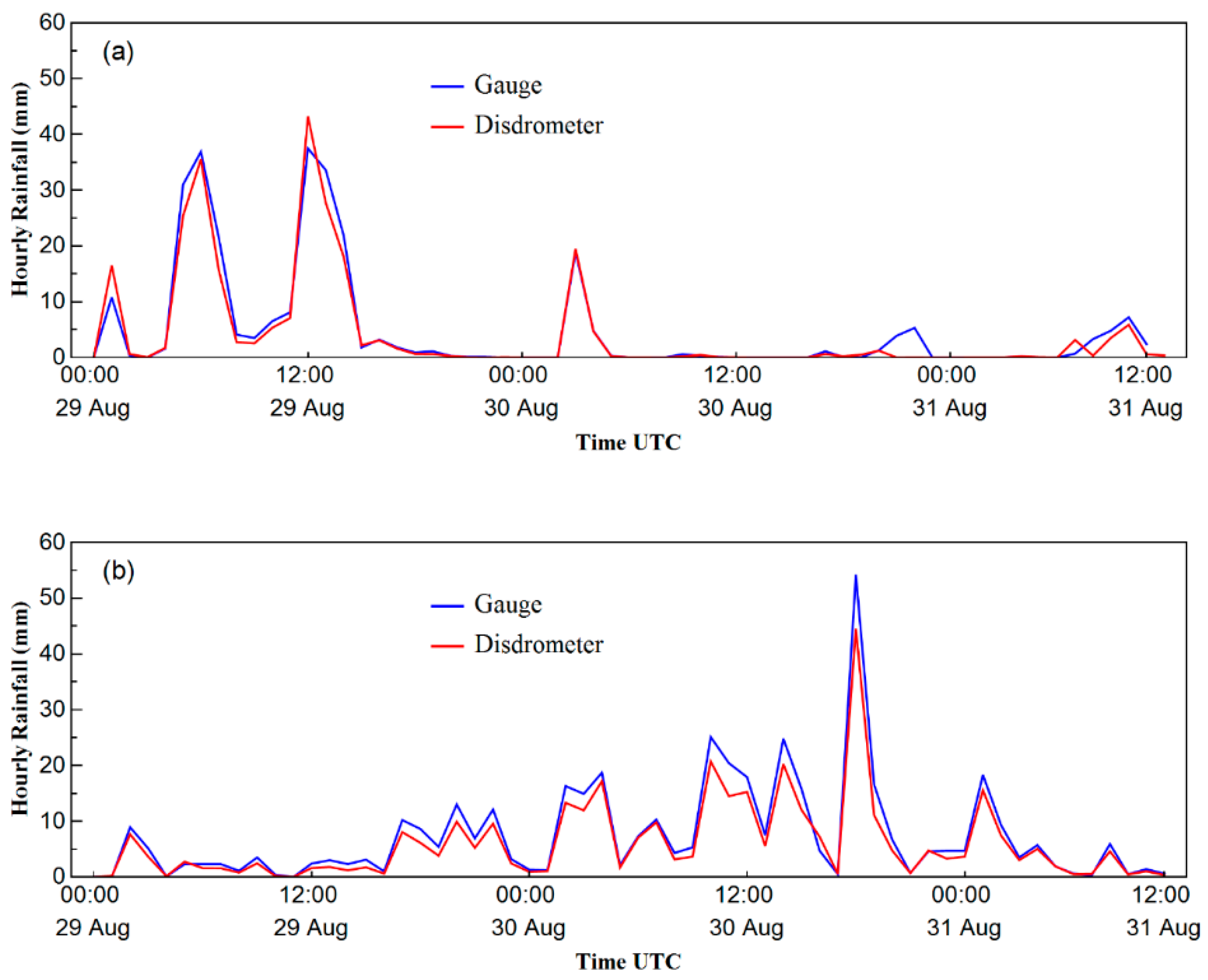
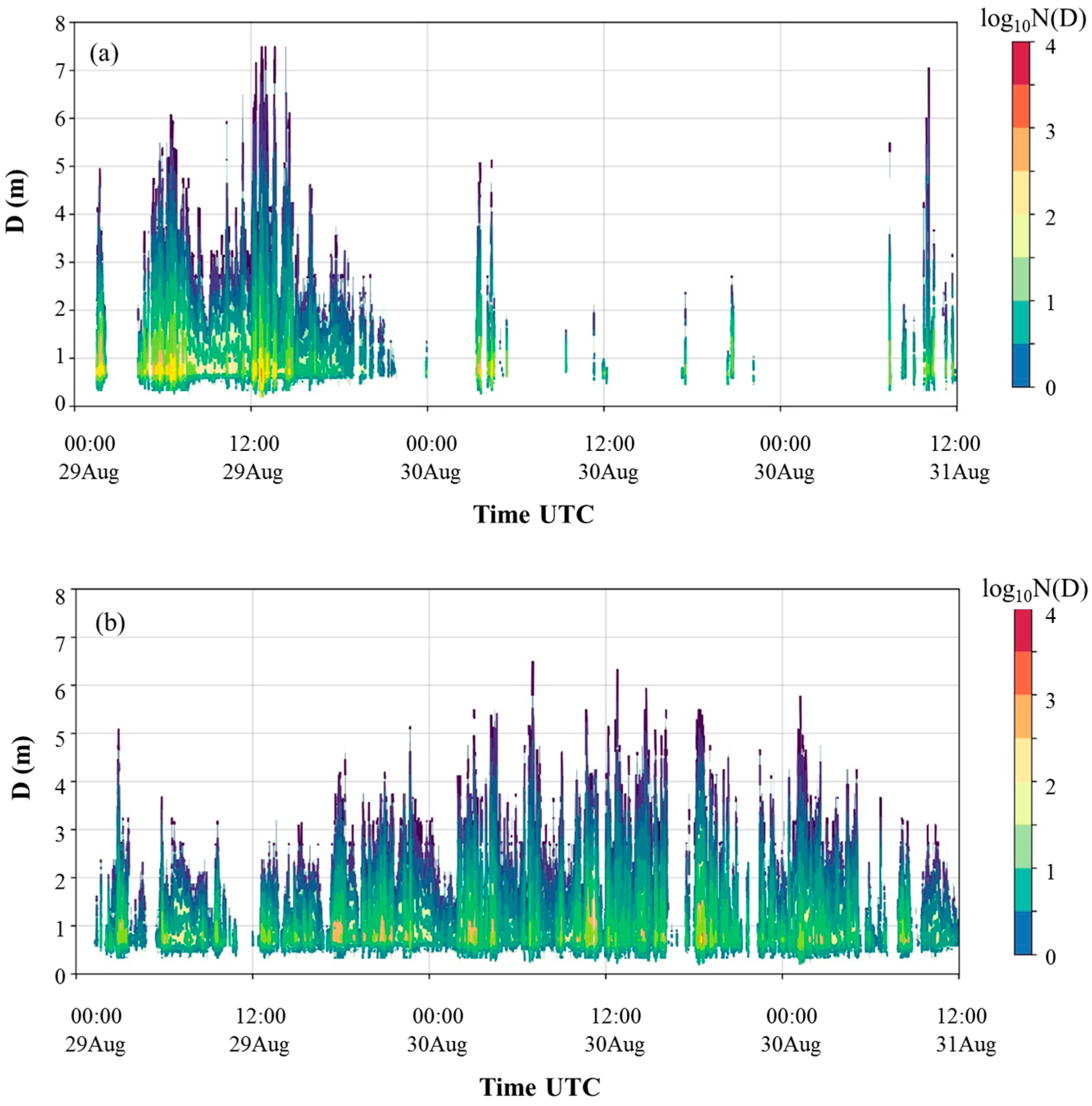
4.2.1. DSDs Time Series at Two Observation Stations

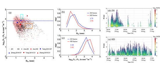
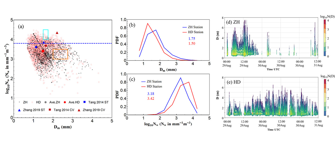
As there are no disdrometers deployed at the Doumen and Gaotan stations, two nearby Parsivel² disdrometers were selected to analyze the raindrop size distribution from 00:00 UTC 29 August to 12:00 UTC 31 August. One disdrometer is located at Zhuhai (22.2750 °N, 113.5669 °E) near the Doumen station (45 km away); the other is located at Huidong (23.0261 °N, 114.6681 °E) near the Gaotan station (67 km away) (see Figure 1). The comparisons of hourly rainfall between the disdrometers and the gauges at Zhuhai and Huidong stations (within 20 m for each pair) are shown in Figure 7. Although the disdrometer might slightly underestimate the rainfall compared with gauge data because of the absence of some records and the overlap of drops along the laser beam, overall, they captured the rainfall pattern very well. As such, we ignored the impact on DSD observations in this study. Moreover, the rainfall pattern at Zhuhai station is similar to that of Doumen station, and the rainfall pattern of Huidong station is similar to Gaotan station. The similar patterns indicate that these two disdrometers could, respectively, represent the DSD characteristic of Doumen and Gaotan stations.

Figure 8 shows the time series of the drop size distribution ($N(D)$: m⁻³ mm⁻¹) in the logarithmic scale from 00:00 UTC 29 August to 12:00 UTC 31 August, derived by the 1-min disdrometer observations at the two stations. In line with the synoptic condition shown in Figure 2, it can be seen that the Zhuhai station experienced stronger rainfall during 29 August, and it reached the maximum hourly rainfall of about 40 mm (Figure 7). The maximum raindrops greater than 7 mm were recorded from 12:00 to 14:00 UTC 29 August. After that, rainfall at Zhuhai station began to weaken with the decreasing number of raindrop concentration and size of raindrops, while that at Huidong station gradually increased. After 23:00 UTC 29 August, this long-lasting storm disappeared at Zhuhai station following with two short storms characterized with lower concentration but bigger raindrops around 04:00 UTC 30 August and around 11:00 UTC 31 August. The rain at Huidong station showed an increasing trend from 13:00 UTC 29 August, and the number of raindrop concentration and size of raindrops also show an increasing trend, and the hourly rainfall reached the highest from 18:00 to 19:00 UTC 30 August. Compared to the extreme rainfall period at Zhuhai station, the number of large drops (D > 5 mm) at Huidong station is much less during the strong rainfall period which we hypothesize is due to the collision caused by sea-inland orographic effect [38,39,40].

4.2.2. The Distribution of $D_m$ and $N_w$

Figure 9a shows the scatterplot of ${\log }_{10}{N}_w$ vs. $D_m$ of the two stations. The maritime convective clusters, continental convective clusters, and the stratiform rain line described in Bringi et al. [41] as well as the convection-stratiform separation line suggested by Thompson et al. [42] are also shown in Figure 9a. The scatter points of two stations show similar boundaries, of which there are both convective rain and stratiform rain types. Meanwhile, there are more points classified as stratiform rain by the classification suggested by Thompson et al. [42], and the averaged ${\log }_{10}{N}_w$-$D_m$ pairs of two stations are close to the stratiform line described by Bringi et al. [41]. Moreover, for convective rain type, there are more points located at the continental convective cluster rather than maritime cluster for both stations. Compared with the DSD characteristics studied at Yangjiang from July to August by Tang et al. [43], the ${\log }_{10}{N}_w$ of both two stations are smaller no matter what rain types, suggesting a lower drop concentration of this rain system.

The probability density functions (PDFs) of $D_m$ and ${\log }_{10}{N}_w$ with the mean values are presented in Figure 9b,c. The PDF of $D_m$ at Zhuhai station peaks around 1.25 mm while that at Huidong peaks around at 1.75 mm. Additionally, the PDF of ${\log }_{10}{N}_w$ at Zhuhai station peaks around 3.25 while that at Huidong peaks around at 3.75. This leads to a higher mean value of $D_m$ (1.75 mm) and lower mean value of ${\log }_{10}{N}_w$ (3.18) at Zhuhai station than those at Huidong station. This result indicates that the rain at Zhuhai station has larger drops, but a lower drop number concentration compared to Huidong station.

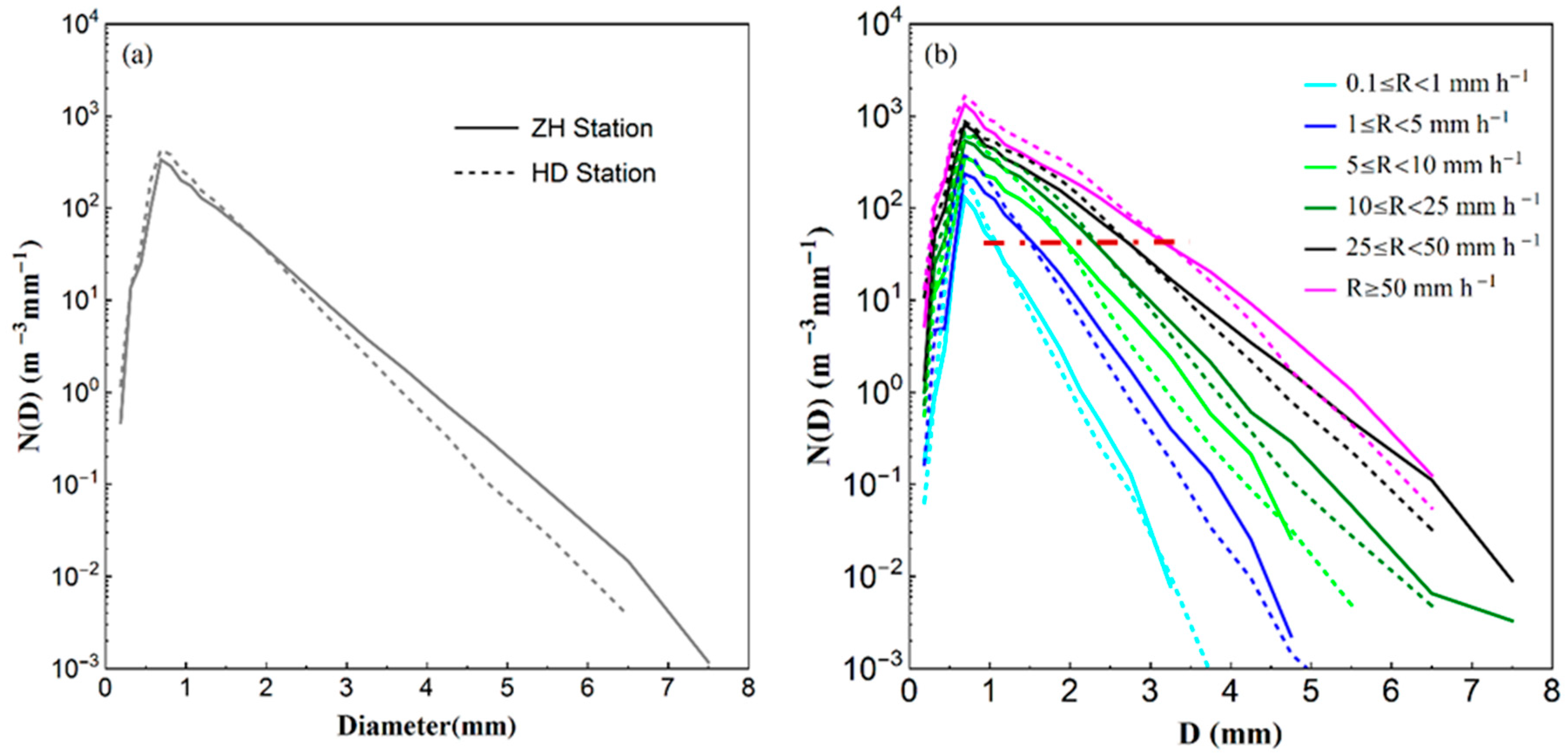
4.2.3. The DSD Spectra

The characteristics of DSD of this rain system are investigated to understand the precipitation microphysical processes. To eliminate to the effect caused by rain rate and duration, the DSD measurements are divided into six classes according to the associated rain rate ($R$): C1,$0.1\le R<1$; C2, $1\le R<5$; C3, $5\le R<10$; C4, $10\le R<25$; C5, $25\le R<50$ mm h⁻¹. Such classification is based on the rain rate distribution of this system, as well as several previous studies [25,35]. The DSD sample relative frequency, rain rate statistics and mean DSD parameters for each class are summarized in

Table 1. Number and DSD retrieved rain rate statistics of each rain rate class for Zhuhai and Huidong station data.

Classes	Rain Rate Threshold (mm h−1)	Relative Frequency		Mean (mm h−1)		SD (mm h−1)		Skewness
		ZH	HD	ZH	HD	ZH	HD	ZH	HD
C1	$0.1\le \mathrm{R}<1$	0.32	0.32	0.52	0.48	0.25	0.26	0.05	0.27
C2	$1\le \mathrm{R}<5$	0.35	0.37	2.66	2.30	1.10	1.04	0.28	0.82
C3	$5\le \mathrm{R}<10$	0.09	0.11	7.41	7.07	1.45	1.44	0.17	0.32
C4	$10\le \mathrm{R}<25$	0.12	0.11	15.72	16.46	4.09	4.16	0.31	0.32
C5	$25\le \mathrm{R}<50$	0.09	0.06	35.41	35.38	6.85	7.30	0.25	0.34
C6	$\mathrm{R}\ge 50$	0.03	0.02	68.14	71.02	12.14	16.40	0.77	0.87
All data	-	1	1	9.01	7.43	15.28	13.81	2.70	3.45

and

Table 2. Mean values DSD parameters for each rain rate class for Zhuhai and Huidong station data.

Classes	${\mathit{D}}_{\mathit{m}}$(mm)		${\mathit{N}}_{\mathit{t}}$(m−3)		${\mathbf{log}}_{\mathbf{10}}{\mathit{N}}_{\mathit{w}}$(m−3 mm−1)		$\mathit{W}$(g m−3)
	ZH	HD	ZH	HD	ZH	HD	ZH	HD
C1	1.29	1.14	54.8	81.0	2.94	3.18	0.030	0.031
C2	1.66	1.43	139.6	200.5	3.19	3.42	0.132	0.127
C3	1.96	1.64	255.2	409.6	3.30	3.67	0.337	0.360
C4	2.18	1.96	429.8	548.5	3.44	3.66	0.682	0.748
C5	2.62	2.32	648.2	786.8	3.44	3.66	1.409	1.474
C6	2.80	2.48	1051.5	1369.3	3.57	3.82	2.616	2.863
All data	1.75	1.50	232.1	286.8	3.18	3.42	0.378	0.337

. For lower rain rate classes (C1–C3), the rain rate of Huidong station is lower than that of Zhuhai station. For C5, the rain rates of two stations are close to each other and for the other two high rain rate classes (C4 and C6), the rain rate of Huidong station is higher than that of Zhuhai station, which caused the higher hourly rainfall at from 18:00 to 19:00 UTC 30 August. However, due to the lower relative frequency of high rain rate classes, the overall average rain rate of Huidong station is smaller than that of Zhuhai station.

It can be shown from Figure 10 that the total averaged DSD of Zhuhai station has wider spread as well as lower concentration at small and medium-sized drops (D < 2 mm) but higher concentration at big and large drops (D > 2 mm) compared with that of Huidong station, which corresponds to a larger$D_m$, more W, but a lower $N_t$ for Zhuhai station compared with those for Huidong station (Table 2). For the same rain class, the DSD of Huidong shows the same characteristics with higher concentration at smaller drops as well as lower concentration at larger drops. Additionally, the diameters where the raindrop concentrations of two stations become larger as the rain classes increased, from 1.2 to 3.8 mm, due to the higher the concentration of larger drops at higher rain rates for both stations.

Table 3. Relative contributions of each size class to the total drop numbers$T_d$, total drop concentration$N_t$, liquid water content $W$, rain rate $R$. The bold number highlights the maximum.

D (mm)	${\mathit{T}}_{\mathit{d}}$ (%)		${\mathit{N}}_{\mathit{t}}$ (%)		$\mathit{R}$ (%)		$\mathit{W}$ (%)
	ZH	HD	ZH	HD	ZH	HD	ZH	HD
<1	38.08	44.26	51.99	57.92	3.91	6.30	7.79	11.69
1~2	47.48	45.99	39.54	36.60	30.70	40.50	37.01	45.65
2~3	11.67	8.41	7.03	4.82	34.39	34.00	31.33	28.83
3~4	2.24	1.16	1.18	0.58	19.22	13.80	15.25	10.16
>4	0.53	0.18	0.26	0.08	11.78	5.40	8.62	3.67

summarizes the relative contributions of each size class to $N_t$, $W$, and $R,$which are obtained through dividing the parameters calculated for the raindrops of each size class by the corresponding parameters calculated for all the size classes. For both stations, the small raindrops (D < 1 mm) have the highest concentration (51.99% and 57.92%) of the total data set and the second highest relative frequency (Td 38.08% and 44.26%), but relatively low contributions to total water content and rainfall. The contribution of small and medium-sized raindrops (D: 1–2 mm) to the total number is the greatest, accounting for 47.48% (45.99%) at Zhuhai (Huidong) station. However, for Zhuhai station, the middle-sized drops (D: 2–3 mm) accounts for the most rainfall (34.39%), while the small and medium-sized raindrops (D: 1–2 mm) account for the most for Huidong station (40.50%). Moreover, for Zhuhai station, the medium-sized and larger drops (D > 2 mm) account more for rainfall and water content compared with Huidong station, as the higher relative frequency. This result is consistent with the conclusion shown in Figure 8 and Figure 9 that larger drops are less likely to occur at Huidong, where complex topography could exacerbate the collision.

4.3. Polarimetric Radar Signatures and Rainfall Analysis

As the rain patterns of Zhuhai station and Huidong station are similar to that of Doumen station and Gaotan station, the DSD characteristics of Zhuhai and Huidong areas can partly represent the microphysics of Doumen and Gaotan station, which suggests a high probability of a higher drop concentration at Gaotan station and a larger drops at Doumen station. However, the total rainfall difference between Huidong and Gaotan station is significant (≈400 mm vs. ≈1000 mm), which means the DSD of Gaotan may be different and need more observation to supplement the current study. In the following study, the dual-polarized radar observations are used to further understand the rainfall.

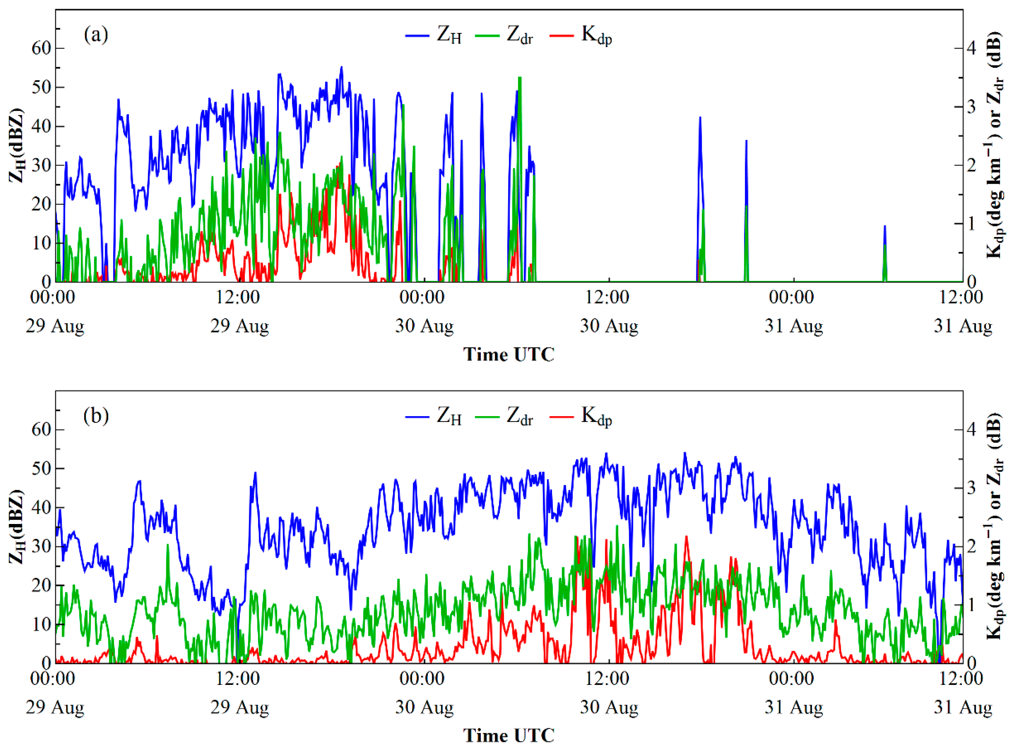
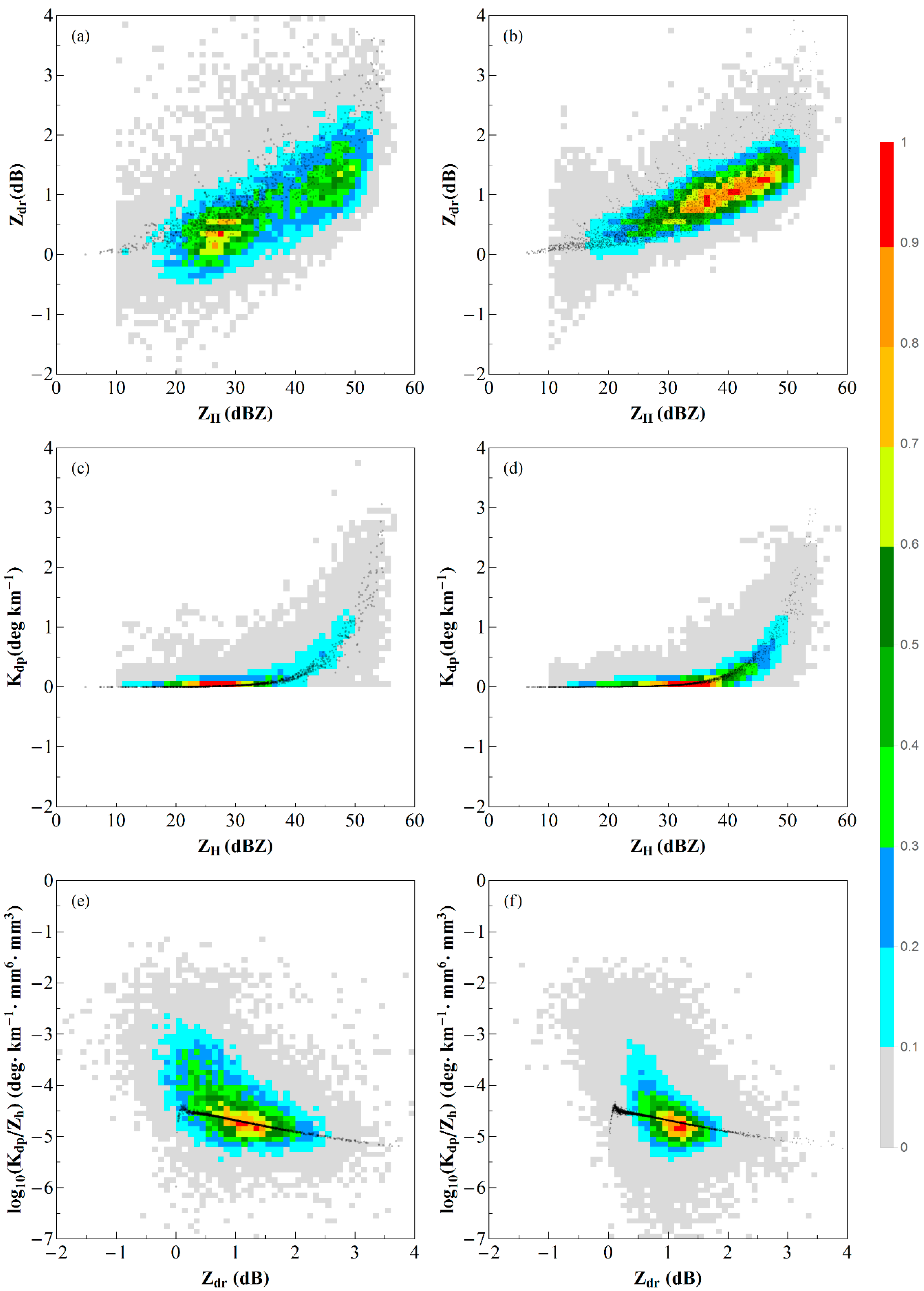
4.3.1. The Polarimetric Radar Signatures

To further understand the differences between the two rain patterns on 29 and 30 August, the polarimetric radar fields over the two extreme stations are compared. Figure 11 shows the time series of polarimetric variables over Doumen and Gaotan stations observed by GZRD and MZRD 0.5-degree sweeps, respectively. The size of radar pixel over Doumen (Gaotan) station is around 0.25 × 1.49 km (0.25 × 2.23 km), and the horizontal/vertical distances are 93 km/0.81 km (137 km/1.21 km) between the radar pixel and the station. Generally speaking, Figure 11 shows that the timing changes of radar variables are consistent with the rainfall changes at both stations (Figure 6). During the extreme rainfall periods of Doumen station and Gaotan station, the mean values of $Z_H$ over both stations are similar while the mean value of $Z_{dr}$ over Doumen station is higher than that over Gaotan station, indicating that bigger drops are more likely to occur at Doumen station than Gaotan station, which is similar to the DSD analysis of Zhuhai and Huidong.

To eliminate the random error of one radar pixel, two extreme regions were defined as circular areas with a radius of 5 km centered on Doumen station and Gaotan station, respectively, hereafter referred to Doumen rain region and Gaotan rain region. The polarimetric variables from 0.5-degree sweep over these two regions from 00:00 UTC 29 August to 12:00 UTC 31 August were analyzed. Figure 12 shows the joint frequency distributions of $Z_{dr}$ vs. $Z_H$, $K_{dp}$ vs. $Z_H$, as well as ${\log }_{10}(K_{dp}/Z_h)$ vs. $Z_{dr}$ observed by radars over two regions as well as the simulated radar moments based on DSD data at Zhuhai station and Huidong station. The frequency at each pair of data bin (e.g., the bin width is 1 dBZ for $Z_H$ and 0.1 dB for$Z_{dr}$, 0.1 degree km⁻¹ for $K_{dp}$, and 0.1 for log₁₀($K_{dp}/Z_h$)) refers to the total number of radar pixels with values of $Z_{dr}$ vs. $Z_H$ ($K_{dp}$ vs. $Z_H$ or ${\log }_{10}(K_{dp}/Z_h)$ vs. $Z_{dr}$) falling into the bins, and the frequency distribution is further normalized by dividing by the maximum frequency among all the pairs of data bins.

Frequencies for the observed $Z_H$,$Z_{dr}$ at Doumen rain region peaked at approximately 28 dBZ, and 0.3 dB, respectively. While at Gaotan rain region they peaked at high values, around 35 dBZ for $Z_H$ and 0.8 dB for $Z_{dr}$. The $Z_H$ maximum values with the 10% normalized frequency of two regions are similar around 52 dBZ, which are consistent with the extreme rainfall periods of two stations. Meanwhile, the $Z_{dr}$ maximum values with the 10% normalized frequency at Gaotan rain region is smaller (2.1 dB vs. 2.5 dB). Meanwhile, for the same $Z_H$, the range and mean$Z_{dr}$ at Doumen rain region is larger than that at Gaotan station, which indicates that larger drops more likely occurred at Doumen compared with Gaotan. For both regions, the slope between $Z_H$ and $K_{dp}$ shows a sharp transition over sampling grids with $Z_H$ exceeding 40 dBZ, resulting in a rapid increase of $K_{dp}$ along with the increase of $Z_H$. Although the peak frequencies for $K_{dp}$ at two rain regions are similar around 0.1 degree km⁻¹, $K_{dp}$ increases faster as the $Z_H$ increases at Doumen rain region which indicates that there are more relative larger drops at Doumen rain region. Then, considering the higher rain rate and smaller raindrops at Gaotan station, the number concentration must be larger. The extreme lower value of ${\log }_{10}(K_{dp}/Z_h)$ could confirm this, which means the concentration of small drops at Gaotan is higher than that at Doumen. It can be concluded from the polarimetric radar signatures that compared with Doumen rain region, the raindrops at Gaotan rain region have higher concentration but smaller drops, which is consistent with the DSD characteristic at Huidong station.

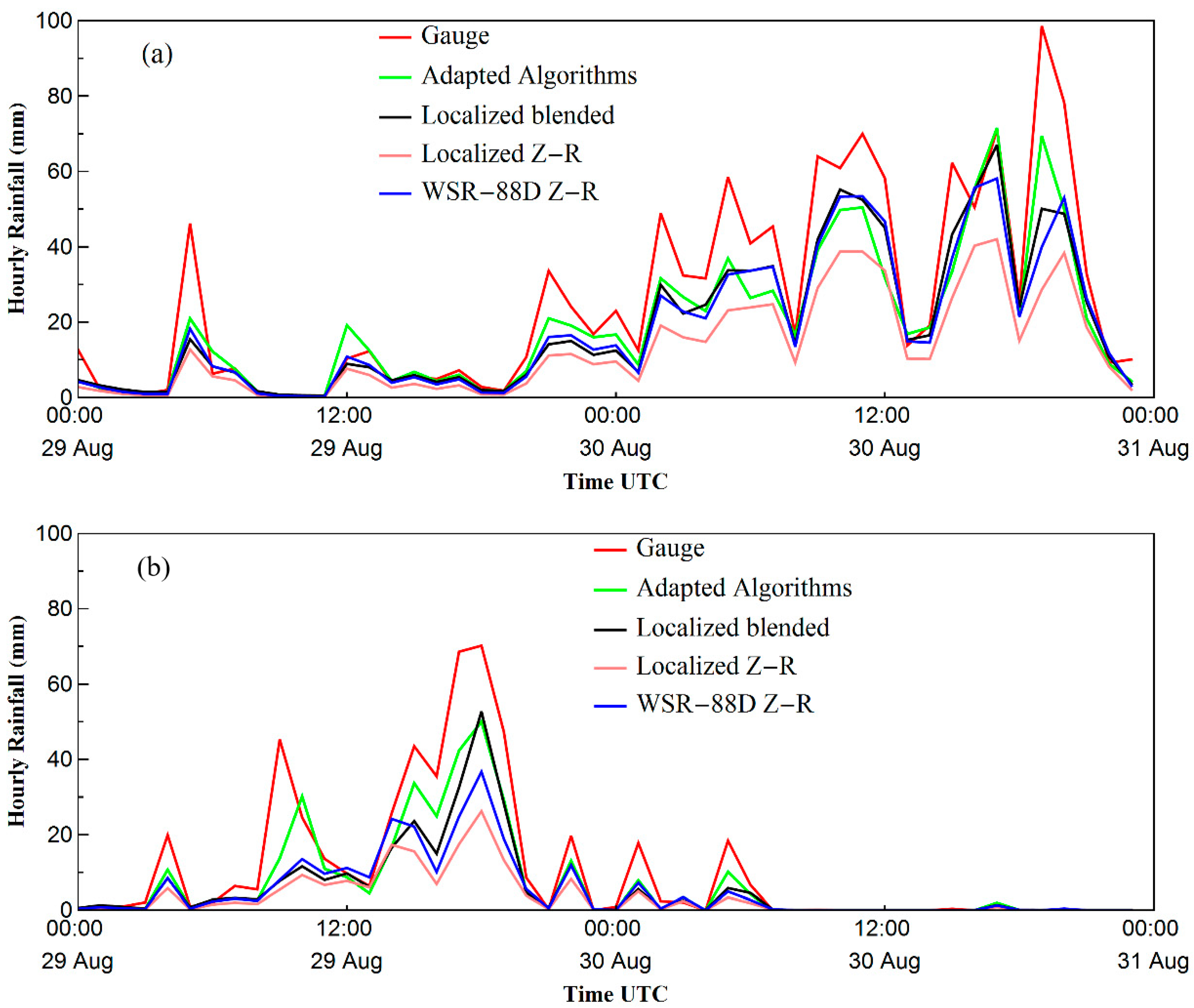
4.3.2. Radar-Based Quantitative Precipitation Estimation (QPE)

In this part, a set of various radar rainfall algorithms including the “adapted algorithm” [36], the localized blended algorithm, the localized relation and WSR-88D Z-R relation [13], were applied to quantify the precipitation intensity and amounts during this event. After estimating the instantaneous rainfall rates using various radar rainfall algorithms, the rainfall accumulations were computed at hourly scale. To quantify the performances of different algorithms, a set of metrics was computed, including the bias (BIAS), normalized mean bias ($NMB$), normalized mean absolute error ($NMAE$), Pearson’s correlation coefficients ($CC$), which are defined as follows:

$$BIAS= \frac{{\sum }_{N=1}^M(R_N - G_N)}{M},$$

(13)

$$NMB = \frac{[{\sum }_{N=1}^M(R_N - G_N)]/M}{({\sum }_{N=1}^M{G}_N)/M}\times 100\%,$$

(14)

$$NMAE = \frac{({\sum }_{N=1}^M|R_N - G_N|)/M}{({\sum }_{N=1}^M{G}_N)/M}\times 100\%,$$

(15)

$$CC = \frac{{\sum }_{N=1}^M(R_N - \overline{R_N})(G_N - \overline{G_N})}{\sqrt{{\sum }_{N=1}^M{(R_N - \overline{R_N})}^2{\sum }_{N=1}^M{(G_N - \overline{G_N})}^2}},$$

(16)

where $R_N$ and $G_N$ represent the radar estimates of different algorithms and the rain gauge measurements at time frame $N$, respectively. $M$ is the total sample number.

The comparison of estimates from different rainfall algorithms and rain gauge measurements at Gaotan and Doumen station is shown in Figure 13 and the evaluation results are shown in

Table 4. Evaluation results of the various radar algorithms at Gaotan station and Doumen station.

Station	Metrics	Algorithm
		“Adapted Algorithm”	Localized Blended Rainfall Algorithm	Localized Z–R Relation	WSR-88D Z-R Relation
Gaotan	BIAS (mm)	−6.61	−7.30	−13.17	−7.90
	NMB (%)	−25.37	−28.01	−50.56	−30.31
	NMAE (%)	29.64	30.16	50.56	32.26
	CC	0.95	0.94	0.93	0.93
Huidong	BIAS (mm)	−3.65	−4.92	−7.03	−5.47
	NMB (%)	−34.39	−46.37	−66.29	−51.63
	NMAE (%)	37.65	47.83	66.72	54.36
	CC	0.96	0.93	0.91	0.91

. As shown in Figure 13, all the algorithms have similar patterns to the rain gauge measurements, while QPE results of the “adapted algorithm” is better than other algorithms with lowest BIAS, NMB, NMAE and the highest CC (Table 4). This is in line with the findings during typhoon case studies [36]. Nevertheless, we should note that all the algorithms are underestimating the rain rates and accumulations during this flood event and the results still need to be optimized.

To further analyze the QPE results of various radar rainfall algorithms, the scatter plots of radar rainfall estimates versus gauge measurements at all rain gauge stations less than 100 km from the radars are shown in Figure 14 and the evaluation results are shown in

Table 5. Evaluation results of the various radar algorithms compared with gauges within 100-km scale of radars.

Metrics	Algorithm
	“Adapted Algorithm”	Localized Blended Rainfall Algorithm	Localized Z–R Relation	WSR-88D Z-R Relation
BIAS (mm)	−0.29	−0.90	−1.38	−1.09
NMB (%)	−12.47	−39.21	−60.35	−47.70
NMAE (%)	39.93	46.38	63.24	53.76
CC	0.91	0.92	0.90	0.90

. Most of the hourly rainfall rates are from 0 to 40 mm hr⁻¹. Again, the adapted algorithm has the best performance, while all the rainfall algorithms show underestimation compared to the gauge measurements, especially during heavy rain periods.

5. Discussion

Although the analysis of DSD and polarimetric radar signatures shows similar results, the relatively long distances between disdrometers and the extreme rain centers might induce some uncertainty in the representation of extreme rainfall DSD characteristics. As mentioned, the polarimetric radar signatures at the two rainfall centers are quite different, even for the same precipitation system, which is likely due to the complex falling processes as a result of orographic enhancement and dynamic cloud microphysics involved in this extreme event [44]. More disdrometers and in situ measurements would be required to fully resolve the three-dimensional structure of precipitation in such complex terrains.

In addition, although the polarimetric radars could provide more insights into the two extreme rain regions, the precipitation estimated by the current radar algorithms underestimate the rainfall compared to the ground gauges. The differences of sample areas between radars and gauges may be one reason, especially when the gauges are far from the radars. In such cases, a network of short-range X-band polarimetric radars would be useful for better QPE. Additionally, the adapted algorithms have relatively better performance mainly because they are derived using DSD and gauge data collected during many storm events in Southern China [36]. However, at the same time, the DSD observed at both Huidong and Zhuhai stations during this event showed a lower number concentration compared with previous long-term studies in Yangjiang [43]. This reminds us that the rainfall algorithms should be appropriately developed based on local rainfall characteristics, which is still under investigation.

6. Conclusions

An epic flood event occurred in southern China from 27 August to 1 September 2018, with a maximum accumulative rainfall of 1394.6 mm recorded at Gaotan station. Multi-observations including reanalysis data, soundings, gauges, disdrometers, and polarimetric radars were used to comprehensively analyze this extreme precipitation event. Based on the reanalysis and gauge data, the synoptic environment and precipitation pattern were investigated. The DSD time series, the mass weighted diameter $D_m$, and normalized intercept parameter $N_w$ of Huidong and Zhuhai stations were derived to achieve a better understanding of the precipitation microphysics. It was found that the depression coupled with land–sea interaction and orographic enhancement kept providing moisture to Guangdong province, leading to the extreme rainfall on 29 at Doumen station and on 30 August at Gaotan station. Although both locations are under the same synoptic system, the DSD observed at Huidong station showed a higher number concentration at smaller drop size and lower number concentration at larger drop size compared with the Zhuhai station. This is likely due to the stronger collision caused by sea–inland orographic effect near the Huidong station, which is similar to the microphysical signatures observed by polarimetric radars at Gaotan and Doumen rain regions. Future study is needed to reveal the mechanism of the sea–inland orographic effect on the precipitation microphysics. In addition, the radar based QPE results show that the rainfall algorithms have great influence on the accuracy. Extra work is required to improve local radar rainfall estimates in order to further help with the severe weather warning operations.

References

1. Stevenson, S.N.; Schumacher, R.S. A 10-Year Survey of Extreme Rainfall Events in the Central and Eastern United States Using Gridded Multisensor Precipitation Analyses. Mon. Weather Rev. 2014, 142, 3147–3162. [Google Scholar] [CrossRef]
2. Zhou, T.; Yu, R.; Chen, H.; Dai, A.; Pan, Y. Summer Precipitation Frequency, Intensity, and Diurnal Cycle over China: A Comparison of Satellite Data with Rain Gauge Observations. J. Clim. 2008, 21, 3997–4010. [Google Scholar] [CrossRef]
3. Battan, L.J. Radar Observation of the Atmosphere; University of Chicago Press: Chicago, IL, USA, 1973. [Google Scholar]
4. Abel, S.J.; Boutle, I.A. An improved representation of the raindrop size distribution for single-moment microphysics schemes. Quart. J. R. Meteor. Soc. 2012, 138, 2151–2162. [Google Scholar] [CrossRef]
5. Tang, G.; Zeng, Z.; Ma, M.; Liu, R.; Wen, Y.; Hong, Y. Can Near-Real-Time Satellite Precipitation Products Capture Rainstorms and Guide Flood Warning for the 2016 Summer in South China? IEEE Geosci. Remote Sens. 2017, 14, 1208–1212. [Google Scholar] [CrossRef]
6. Huang, Y.; Liu, Y.; Liu, Y.; Knievel, J.C. Budget Analyses of a Record-Breaking Rainfall Event in the Coastal Metropolitan City of Guangzhou, China. J. Geophys. Res. Atmos. 2019, 124, 9391–9406. [Google Scholar] [CrossRef]
7. Li, H.; Wan, Q.; Peng, D.; Liu, X.; Xiao, H. Multiscale analysis of a record-breaking heavy rainfall event in Guangdong, China. Atmos. Res. 2020, 232, 104703. [Google Scholar] [CrossRef]
8. Chen, X.; Zhao, K.; Xue, M. Spatial and temporal characteristics of warm season convection over Pearl River Delta region, China, based on 3 years of operational radar data. J. Geophys. Res. Atmos. 2014, 119, 412–447. [Google Scholar] [CrossRef]
9. Fu, S.; Li, D.; Sun, J.; Si, D.; Ling, J.; Tian, F. A 31-year trend of the hourly precipitation over South China and the underlying mechanisms. Atmos. Sci. Lett. 2016, 17, 216–222. [Google Scholar] [CrossRef]
10. Li, Z.; Yang, D.; Hong, Y. Multi-scale evaluation of high-resolution multi-sensor blended global precipitation products over the Yangtze River. J. Hydrol. 2013, 500, 157–169. [Google Scholar] [CrossRef]
11. Ma, Y.; Zhang, Y.; Yang, D.; Farhan, S.B. Precipitation bias variability versus various gauges under different climatic conditions over the Third Pole Environment (TPE) region. Int. J. Climatol. 2015, 35, 1201–1211. [Google Scholar] [CrossRef]
12. Wang, Z.; Zhong, R.; Lai, C.; Chen, J. Evaluation of the GPM IMERG satellite-based precipitation products and the hydrological utility. Atmos. Res. 2017, 196, 151–163. [Google Scholar] [CrossRef]
13. Fulton, R.A.; Breidenbach, J.P.; Seo, D.; Miller, D.A.; O’Bannon, T. The WSR-88D Rainfall Algorithm. Weather Forecast 1998, 13, 377–395. [Google Scholar] [CrossRef]
14. Bringi, V.N.; Chandrasekar, V. Polarimetric Doppler Weather Radar: Principles and Applications; Cambridge University Press: Cambridge, UK, 2001. [Google Scholar]
15. Bechini, R.; Chandrasekar, V. A Semisupervised Robust Hydrometeor Classification Method for Dual-Polarization Radar Applications. J. Atmos. Ocean. Tech. 2015, 32, 22–47. [Google Scholar] [CrossRef]
16. Park, H.S.; Ryzhkov, A.V.; Zrnić, D.S.; Kim, K. The Hydrometeor Classification Algorithm for the Polarimetric WSR-88D: Description and Application to an MCS. Weather Forecast 2009, 24, 730–748. [Google Scholar] [CrossRef]
17. Wen, G.; Chen, H.; Zhang, G.; Sun, J. An Inverse Model for Raindrop Size Distribution Retrieval with Polarimetric Variables. Remote Sens. 2018, 10, 1179. [Google Scholar] [CrossRef] [Green Version]
18. Sun, Y.; Xiao, H.; Yang, H.; Feng, L.; Chen, H.; Luo, L. An Inverse Mapping Table Method for Raindrop Size Distribution Parameters Retrieval Using X-band Dual-Polarization Radar Observations. IEEE Trans. Geosci. Remote Sens. 2020, 1–22. [Google Scholar] [CrossRef]
19. Ryzhkov, A.V.; Giangrande, S.E.; Schuur, T.J. Rainfall Estimation with a Polarimetric Prototype of WSR-88D. J. Appl. Meteorol. 2005, 44, 502–515. [Google Scholar] [CrossRef] [Green Version]
20. Berne, A.; Jaffrain, J.; Schleiss, M. Scaling analysis of the variability of the rain drop size distribution at small scale. Adv. Water Resour. 2012, 45, 2–12. [Google Scholar] [CrossRef]
21. McFarquhar, G.M.; Hsieh, T.; Freer, M.; Mascio, J.; Jewett, B.F. The Characterization of Ice Hydrometeor Gamma Size Distributions as Volumes in N0–λ–μ Phase Space: Implications for Microphysical Process Modeling. J. Atmos. Sci. 2015, 72, 892–909. [Google Scholar] [CrossRef]
22. Kalnay, E. The NCEP/NCAR Reanalysis 40-year Project. B. Am. Meteorol. Soc. 1996, 77, 437–471. [Google Scholar] [CrossRef] [Green Version]
23. Tokay, A.; Wolff, D.B.; Petersen, W.A. Evaluation of the New Version of the Laser-Optical Disdrometer, OTT Parsivel2. J. Atmos. Ocean. Technol. 2014, 31, 1276–1288. [Google Scholar] [CrossRef]
24. Löffler-Mang, M.; Joss, J. An Optical Disdrometer for Measuring Size and Velocity of Hydrometeors. J. Atmos. Ocean. Tech. 2000, 17, 130–139. [Google Scholar] [CrossRef]
25. Ma, Y.; Ni, G.; Chandra, C.V.; Tian, F.; Chen, H. Statistical characteristics of raindrop size distribution during rainy seasons in the Beijing urban area and implications for radar rainfall estimation. Hydrol. Earth Syst. Sci. 2019, 23, 4153–4170. [Google Scholar] [CrossRef] [Green Version]
26. Luo, L.; Xiao, H.; Yang, H.; Chen, H.; Guo, J.; Sun, Y.; Feng, L. Raindrop size distribution and microphysical characteristics of a great rainstorm in 2016 in Beijing, China. Atmos. Res. 2020, 239, 104895. [Google Scholar] [CrossRef]
27. Janapati, J.; Seela, B.K.; Reddy, M.V.; Reddy, K.K.; Lin, P.; Rao, T.N.; Liu, C. A study on raindrop size distribution variability in before and after landfall precipitations of tropical cyclones observed over southern India. J. Atmos. Sol. Terr. Phys. 2017, 159, 23–40. [Google Scholar] [CrossRef]
28. Seo, B.; Krajewski, W.F.; Quintero, F.; El Saadani, M.; Goska, R.; Cunha, L.K.; Dolan, B.; Wolff, D.B.; Smith, J.A.; Rutledge, S.A.; et al. Comprehensive Evaluation of the IFloodS Radar Rainfall Products for Hydrologic Applications. J. Hydrometeorol. 2018, 19, 1793–1813. [Google Scholar] [CrossRef]
29. Atlas, D.; Srivastava, R.C.; Sekhon, R.S. Doppler radar characteristics of precipitation at vertical incidence. Rev. Geophys. 1973, 11, 1–35. [Google Scholar] [CrossRef]
30. Jaffrain, J.; Berne, A. Experimental Quantification of the Sampling Uncertainty Associated with Measurements from PARSIVEL Disdrometers. J. Hydrometeorol. 2010, 12, 352–370. [Google Scholar] [CrossRef]
31. Leinonen, J. High-level interface to T-matrix scattering calculations: Architecture, capabilities and limitations. Opt. Express 2014, 22, 1655. [Google Scholar] [CrossRef]
32. Mackowski, D.W.; Mishchenko, M.I. A multiple sphere T-matrix Fortran code for use on parallel computer clusters. J. Quant. Spectrosc. Radiat. Transf. 2011, 112, 2182–2189. [Google Scholar] [CrossRef]
33. Waterman, P.C. Matrix formulation of electromagnetic scattering. Proc. IEEE 1965, 53, 805–812. [Google Scholar] [CrossRef]
34. Thurai, M.; Huang, G.J.; Bringi, V.N.; Randeu, W.L.; Schönhuber, M. Drop Shapes, Model Comparisons, and Calculations of Polarimetric Radar Parameters in Rain. J. Atmos. Ocean. Technol. 2007, 24, 1019–1032. [Google Scholar] [CrossRef]
35. Jash, D.; Resmi, E.A.; Unnikrishnan, C.K.; Sumesh, R.K.; Sreekanth, T.S.; Sukumar, N.; Ramachandran, K.K. Variation in rain drop size distribution and rain integral parameters during southwest monsoon over a tropical station: An inter-comparison of disdrometer and Micro Rain Radar. Atmos. Res. 2019, 217, 24–36. [Google Scholar] [CrossRef]
36. Xia, Q.; Zhang, W.; Chen, H.; Lee, W.-C.; Han, L.; Ma, Y.; Liu, X. Quantification of Precipitation Using Polarimetric Radar Measurements during Several Typhoon Events in Southern China. Remote Sens. 2020, 12, 2058. [Google Scholar] [CrossRef]
37. Weisman, M.L.; Klemp, J.B.; Rotunno, R. Structure and Evolution of Numerically Simulated Squall Lines. J. Atmos. Sci. 1988, 45, 1990–2013. [Google Scholar] [CrossRef] [Green Version]
38. Yang, L.; Smith, J.; Liu, M.; Baeck, M.L. Extreme rainfall from Hurricane Harvey (2017): Empirical intercomparisons of WRF simulations and polarimetric radar fields. Atmos. Res. 2019, 223, 114–131. [Google Scholar] [CrossRef]
39. Powell, M.D. Changes in the low-level kinematic and thermodynamic structure of hurricane Alicia (1983) at landfall. Mon. Weather Rev. 1987, 115, 75–99. [Google Scholar] [CrossRef] [Green Version]
40. Cifelli, R.; Chandrasekar, V.; Chen, H.; Johnson, L.E. High resolution radar quantitative precipitation estimation in the San Francisco Bay Area: Rainfall monitoring for the urban environment. J. Meteorol. Soc. Jpn. Ser. II 2018, 96A, 141–155. [Google Scholar] [CrossRef] [Green Version]
41. Bringi, V.N.; Chandrasekar, V.; Hubbert, J.; Gorgucci, E.; Randeu, W.L.; Schoenhuber, M. Raindrop size distribution in different climatic regimes from disdrometer and dual-polarized radar analysis. J. Atmos. Sci. 2003, 60, 354–365. [Google Scholar] [CrossRef]
42. Thompson, E.J.; Rutledge, S.A.; Dolan, B.; Thurai, M. Drop size distributions and radar observations of convective and stratiform rain over the equatorial Indian and West Pacific Oceans. J. Atmos. Sci. 2015, 72, 4091–4125. [Google Scholar] [CrossRef]
43. Tang, Q.; Xiao, H.; Guo, C.; Feng, L. Characteristics of the raindrop size distributions and their retrieved polarimetric radar parameters in northern and southern China. Atmos. Res. 2014, 135–136, 59–75. [Google Scholar] [CrossRef]
44. Chen, H.; Cifelli, R.; White, A. Improving operational radar rainfall estimates using profiler observations over complex terrain in Northern California. IEEE Trans. Geosci. Remote Sens. 2020, 58, 1821–1832. [Google Scholar] [CrossRef]
Figure 1. The topography of Guangdong province and geographical locations of instruments used in this study. The red circles are the 150-km coverage range rings from the radars. The red square, triangle, star, and pentagon represent the locations of radar, disdrometer, special gauge, and sounding, respectively. The small black circles stand for the gauges. The instrument names are abbreviated version of location names: DM (Doumen), GT (Gaotan), HD (Huidong), QY (Qingyang), ST (Shantou), ZH (Zhuhai).
Remotesensing 12 02772 g001
Figure 2. Geopotential height (gpm, solid blue lines at intervals of 10 gpm), winds (m s−1, black vector arrows, vector scale at upper right), and vorticity (shaded, ×10−4 s−1) at 500 hPa (a) at 12:00 UTC 29 August, and (b) at 12:00 UTC 30 August. The red (blue) shadings in panels (a,b) indicate positive (negative) vorticity. Geopotential height (gpm, solid blue lines at intervals of 10 gpm), winds (m s−1, black vector arrows, vector scale at upper right), and the temperature advection (shaded, ×10−4 °C s−1) at 850 hPa (c) at 12:00 UTC 29 August, and (d) at 12:00 UTC 30 August. The red (blue) shadings in panels (c) and (d) indicate warm (cold) temperature advection. The 1000–300 hPa vertically integrated water vapor transport (IVT, shaded, kg m−1s−1, also in black vector arrows, vector scale at upper right) (e) at 12:00 UTC 29 August, and (f) at 12:00 UTC 30 August. The dashed red rectangle indicates the area of the southeast of Guangdong province.
Remotesensing 12 02772 g002
Figure 3. The skew T-log10P sounding profiles at (a,b) QY station and (c,d) ST station at 1200 UTC 29 August (left) and 1200 UTC 30 August (right). The red dashed line and black and blue solid lines represent the stratification curve, temperature profile, and dew point profile, respectively.
Remotesensing 12 02772 g003
Figure 4. The spatial distribution of the accumulated rainfall from 27 August 2018 to 1 September 2018 of Guangdong province. The red squares and triangles represent the locations of radars and disdrometers, respectively.
Remotesensing 12 02772 g004
Figure 5. Daily rainfall accumulation (in mm, a day is defined from 0000 UTC to 0000 UTC of the next day) for (a) 28 August, (b) 29 August, (c) 30 August, (d) 31 August, (e) a zoomed area for 30 August, (f) a zoomed area for 29 August. Each dot represents a gauge station with daily rainfall accumulation exceeding 100 mm.
Remotesensing 12 02772 g005
Figure 6. Hourly and accumulated precipitation at (a) Doumen station, (b) Gaotan station from 00:00 UTC 29 August to 12:00 UTC 31 August.
Remotesensing 12 02772 g006
Figure 7. Hourly rainfall measured by gauges and collocated disdrometers: (a) Zhuhai station, (b) Huidong station from 00:00 UTC 29 August to 12:00 UTC 31 August.
Remotesensing 12 02772 g007
Figure 8. Time series of raindrop size distributions (DSD) observed at (a) Zhuhai station, (b) Huidong station from 00:00 UTC 29 August to 12:00 UTC 31 August. The color density in both (a) and (b) represents the number concentration in logarithmic units of N ( D ) (m−3 mm−1).
Remotesensing 12 02772 g008
Figure 9. (a) The scatterplots of log 10 N w vs. D m ; (b) probability density functions (PDFs) of D m ; (c) PDFs of log 10 N w at Huidong and Zhuhai stations. Both data are from 00:00 UTC 29 August to 12:00 UTC 31 August. The black dot and pink circle represent Zhuhai data and Huidong data, respectively. The mean values of log10 N w and D m are represented by circles (gray for Zhuhai and red for Huidong). The two rectangles correspond to the maritime (cyan) and continental convective (orange) clusters reported by Bringi et al. [41]. The black and purple dash-dot lines represent the characteristics of stratiform rain described in Bringi et al. [41] and the convection/stratiform separation line from Thompson et al. [42], respectively. The square symbols represent the average values of various types of rain, from Tang et al. [43]. CV stands for convective rain, ST is stratiform rain. ZH is short for Zhuhai, and HD is short for Huidong. It is the same in the following figures and tables.
Remotesensing 12 02772 g009
Figure 10. Mean DSDs observed at Zhuhai and Huidong stations from 00:00 UTC 29 August to 12:00 UTC 31 August: (a) all DSD data, (b) DSD data classified by different rain rates. The solid and dashed lines in (a) and (b) represent Zhuhai and Huidong stations, respectively. The dash-dot line in (b) shows the DSD intersection of two stations for each rain rate class.
Remotesensing 12 02772 g010
Figure 11. Time series of different polarimetric radar variables over (a) Doumen station observed by GZRD, (b) Gaotan station observed by MZRD from 00:00 UTC 29 August to 12:00 UTC 31 August.
Remotesensing 12 02772 g011
Figure 12. Joint frequency distributions of polarimetric radar at (a,c,e) Doumen and (b,d,f) Gaotan areas from 00:00 UTC 29 August to 00:00 UTC 31 August: (a,b) Z d r vs. Z H , (c,d) K d p vs. Z H , (e,f) log 10 ( K d p / Z h ) vs. Z d r . The black dots are the simulated radar moments based on DSD data at (a,c,e) Zhuhai station, (b,d,f) Huidong station.
Remotesensing 12 02772 g012
Figure 13. The rain gauge measurements (red line) and estimates computed by various radar algorithms. (a) Gaotan station, (b) Doumen station.
Remotesensing 12 02772 g013
Figure 14. The scatter plots of radar estimated rainfall versus gauge measurements at gauge locations less than 100 km from the radar: (a) the “adapted algorithm” [36]; (b) localized blended rainfall algorithm; (c) localized Z–R relation; (d) WSR-88D Z-R relation [13]. The color density represents the observation sample numbers in logarithmic unit.
Remotesensing 12 02772 g014