Validation and Evaluation of a Ship Echo-Based Array Phase Manifold Calibration Method for HF Surface Wave Radar DOA Estimation and Current Measurement

Abstract

Shore-based phased-array HF radars have been widely used for remotely sensing ocean surface current, wave, and wind around the world. However, phase uncertainties, especially phase distortions, in receiving elements significantly degrade the performance of beam forming and direction-of-arrival (DOA) estimation for phased-array HF radar. To address this problem, the conventional array signal model is modified by adding a direction-based phase error matrix. Subsequently, an array phase manifold calibration method using antenna responses of incoming ship echoes is proposed. Later, an assessment on the proposed array calibration method is made based on the DOA estimations and current measurements that are obtained from the datasets that were collected with a multi-frequency HF (MHF) radar. MHF radar-estimated DOAs using three calibration strategies are compared with the ship directions that are provided by an Automatic Identification System (AIS). Additionally, comparisons between the MHF radar-derived currents while using three calibration strategies and Acoustic Doppler Current Profilers (ADCP)-measured currents are made. The results indicate that the proposed array calibration method is effective in DOA estimation and current measurement for phased-array HF radars, especially in the phase distortion situation.

1. Introduction

Up to now shore-based HF surface wave radars, which operate in the band from 3–30 MHz, have been extensively used for ocean surface current [1], wave [2], and wind measurement [3], as well as ship detection [4,5,6]. The capability of obtaining ocean parameters with a relatively high temporal resolution and a fairly extensive coverage makes HF radars suitable for oceanography research [7], hazard forecasting [8], coastal engineering [9], and maritime security [10,11]. Many types of HF radars are in operation worldwide [12,13,14]. Estimating the range and bearing from the backscattering patch to the receiving antennas is a necessary step for a HF radar to map ocean surface currents [15]. The distance from the backscattering patch to the radar is quite easy to estimate, whereas the estimation of target bearing is much more complicated. Direction-finding and beam-forming methods have been commonly adopted to estimate the direction-of-arrival (DOA) of the sea echo for HF radars [16]. For example, direction-finding techniques, such as multiple signal classification (MUSIC) algorithm, have been used by the Seasonde HF radar and the multi-frequency HF (MHF) radar to determine DOAs of sea surface current echoes. Kirincich et al. recently compared the performance of different direction-finding methods for HF radar current measurements [17]. In contrast, the WavE RAdar (WERA), which takes advantage of a long receiving array, adopts the beam-forming method to steer in the desired direction. However, in practical situations, both of the approaches are negatively affected by array uncertainties [18]. Without array calibration, the beam-forming method may result in an incorrect beam with a broadened beamwidth, and the direction-finding approach would yield a spurious direction with a poor angular resolution [19,20,21].

Unlike the use of array amplitude pattern in direction-finding HF radars [22], the performance of a phased-array HF radar significantly depends on the accuracy of the phase differences (or time delay) among receiving elements [23]. Cost-effective and real-time array calibration methods for phased-array HF radars have received significant attention in the past several years. For example, Fabrizio et al. developed an adaptive algorithm that estimates the receiver frequency response corrections for HF radar arrays [24]. Later, a maximum-likelihood (ML)-based phase error calibration method in which sea echoes are regarded as disparate sources was developed for the Ocean State Monitor and Analysis Radar (OSMAR) [25]. Afterwards, Fernandez et al. developed a phase error calibration method treating ship echoes as disparate sources [26]. Subsequently, Flores-Vidal et al. employed a number of unknown ship echoes to solve the phase errors from a cost function [27]. Recently, Chen et al. developed an approach that is based on the MUSIC algorithm (so-called MU method) for calibrating phase errors while using single-DOA sea echoes [28], and this method was compared with the ML-based method based on current measurements [18]. Almost all of the aforementioned methods only consider the phase uncertainty for each receiving element as a constant value that does not vary with direction. However, phase distortion in the receiving elements [29,30], which has a negative impact on the radar performance, is neglected in the aforementioned methods. This phase distortion problem was recently found in a small-aperture HF radar based on a circular array [31].

In order to address the phase distortion problem, the conventional array signal model is modified by adding a direction-based phase error matrix, and a new array phase manifold calibration method using measured phase responses of incoming ship echoes is proposed to compensate the array phase distortions. An assessment on the proposed array calibration method is made based on the DOA estimations and current measurements that are obtained from the datasets collected by a multi-frequency HF (MHF) radar, especially in the phase distortion case. The paper is organized, as follows: Section 2 contains the array signal model and a modified array signal model. The array phase manifold calibration method and DOA estimation method are also presented in this section. A description of the MHF radar and an example of array phase manifold measurement are given in Section 3. The assessment on the proposed calibration method based on DOA estimations and current measurements is provided in Section 4. The results are discussed in Section 5. Section 6 consists of a conclusion.

2. Calibration Model and Method

2.1. Conventional Calibration Model

Consider a narrowband signal $s\left(t\right)$ with a DOA of $\theta$ observed by a receiving array consisting of M elements, in the absence of the mutual coupling, the signal at the output of the mth antenna element [28], $z_m$, can be described by

$$z_m\left(t\right)={\mathrm{g}}_m{e}^{j{\varphi }_m}{e}^{j\omega {\tau }_m}s\left(t\right)+n_m\left(t\right),$$

(1)

where the subscript m denotes the mth antenna element, t represents time, $g_m=1+{\alpha }_m$, ${\alpha }_m$ and ${\varphi }_m$ are the gain and phase errors, respectively, $\omega$ denotes the radar operating radian frequency, ${\tau }_m=\left(x_{m}sin\theta +y_{m}cos\theta \right)/c$ represents the time delay of radio wave, $\left(x_m,y_m\right)$ defines the position of the mth antenna element for a planar array, c represents the speed of light in free space, and $n_m\left(t\right)$ is the additive receiver noise.

Let $A_m=e^{j\omega {\tau }_m}$, then the output vector $\mathit{Z}\left(t\right)$ of M antenna elements can be expressed while using vector notation as

$$\mathit{Z}\left(t\right)=\mathbf{\Phi }\mathit{A}s\left(t\right)+\mathit{N}\left(t\right),$$

(2)

where $\mathit{Z}\left(t\right)={[z_1\left(t\right),z_2\left(t\right),\cdots ,z_M\left(t\right)]}^T$, T is the transpose operator, $\mathbf{\Phi }=\mathrm{diag}\left\{[g_1{e}^{j{\varphi }_1},g_2{e}^{j{\varphi }_2},\cdots ,g_M{e}^{j{\varphi }_M}]\right\}$ represents the gain and phase error matrix, $\mathit{A}={\left[A_1,A_2,\cdots ,A_M\right]}^T$ denotes the steering vector, and $\mathit{N}\left(t\right)={[n_1\left(t\right),n_2\left(t\right),...,n_M\left(t\right)]}^T$ represents the additive noise vector.

In this model, the gain and phase errors are assumed to be constant for each antenna element. The model has been widely used for phased-array HF radars. Some aforementioned methods, e.g., [27,28], have been developed to estimate the gain and phase errors. For this model, it is straightforward to compensate the received signals if the gain and phase errors $\mathbf{\Phi }$ have been estimated. Subsequently, the output vector of M antenna elements becomes

$$\mathit{Z}\left(t\right)=\mathit{A}s\left(t\right)+\mathit{N}\left(t\right).$$

(3)

From the output vector, the DOA of the radar returns can be estimated using a direction-finding approach [1]. Actually, the phase distortion exists in the receiving elements. Figure 1 shows an example of the phase values of $A_m$ measured from an MHF radar operating at 16.8 MHz. In Figure 1, the red lines, which are simulated using (3) from the receiving array configuration of MHF radar (see Figure 2), denote the ideal phase values against the signal direction. In contrast, the blue dots, which are measured from the known ship echoes that were collected with the MHF radar, represent the measured phase values. If there is no phase distortion, the correlation coefficient (CC) between the ideal phase values and the measured phase values should be 1. However, the CCs for antenna 3 and antenna 4 are 0.76 and 0.89, respectively. Obviously, there are some differences between the ideal and the measured phase values, and this difference is a function of direction.

2.2. Modified Calibration Model

The phase distortion leads the phase differences in Figure 1, and the gain and phase errors vary with direction in the presence of phase distortions. Consequently, the array signal model in (1) for a source signal coming from $\theta$ should be modified using direction-based gain and phase errors as

$$z_m\left(t\right)={\mathrm{g}}_m\left(\theta \right)e^{j{\varphi }_m\left(\theta \right)}{e}^{j\omega {\tau }_m}s\left(t\right)+n_m\left(t\right).$$

(4)

Subsequently, the output vector of M antenna elements in (2) can be expressed as

$$\mathit{Z}\left(t\right)=\mathbf{\Phi }\left(\theta \right)\mathit{A}\left(\theta \right)s\left(t\right)+\mathit{N}\left(t\right),$$

(5)

where the gain and phase error matrix $\mathbf{\Phi }\left(\theta \right)$ is a function of $\theta$ and $\mathbf{\Phi }\left(\theta \right)=\mathrm{diag}\left\{[g_1\left(\theta \right)e^{j{\varphi }_1\left(\theta \right)},\cdots ,g_M\left(\theta \right)e^{j{\varphi }_M\left(\theta \right)}]\right\}$.

It can be found from (4) that, for a given $\theta$, the value

$$B_m\left(\theta \right)=\frac{e^{j\left({\varphi }_m\left(\theta \right)+\omega {\tau }_m\right)}}{e^{j({\varphi }_1\left(\theta \right)+\omega {\tau }_1)}}$$

(6)

is constant. Let the first antenna element be a referenced element, then (4) could be expressed as

$$z_m\left(t\right)={\mathrm{g}}_m\left(\theta \right)B_m\left(\theta \right)e^{j({\varphi }_1\left(\theta \right)+\omega {\tau }_1)}s\left(t\right)+n_m\left(t\right),$$

(7)

and $z_1$ becomes

$$z_1\left(t\right)={\mathrm{g}}_1\left(\theta \right)B_1{e}^{j({\varphi }_1\left(\theta \right)+\omega {\tau }_1)}s\left(t\right)+n_1\left(t\right),$$

(8)

where $B_1=1$. From (7) and (8), the output vector of M antenna elements in (5) becomes

$$\mathit{Z}\left(t\right)=\mathit{B}\left(\theta \right)e^{j({\varphi }_1\left(\theta \right)+\omega {\tau }_1)}s\left(t\right)+\mathit{N}\left(t\right),$$

(9)

where $\mathit{B}={[g_1{B}_1,g_2{B}_2,\cdots ,g_M{B}_M]}^T$ denotes the array phase manifold or the new steering vector. The gain and phase errors in (5) are associated with direction, and the bearing of the incoming signal is unknown. Therefore, it is impossible to directly compensate the received signal to obtain the signals in (5). Alternatively, the term $\mathit{B}\left(\theta \right)$ can be treated as a steering vector and estimated while using the responses of receiving antenna array. If the phase of $\mathit{B}\left(\theta \right)$ is measured (like the blue dots in Figure 1), the $\mathit{B}\left(\theta \right)$ can be calculated and then used to estimate a more accurate DOA rather than using the term $\mathit{A}\left(\theta \right)$.

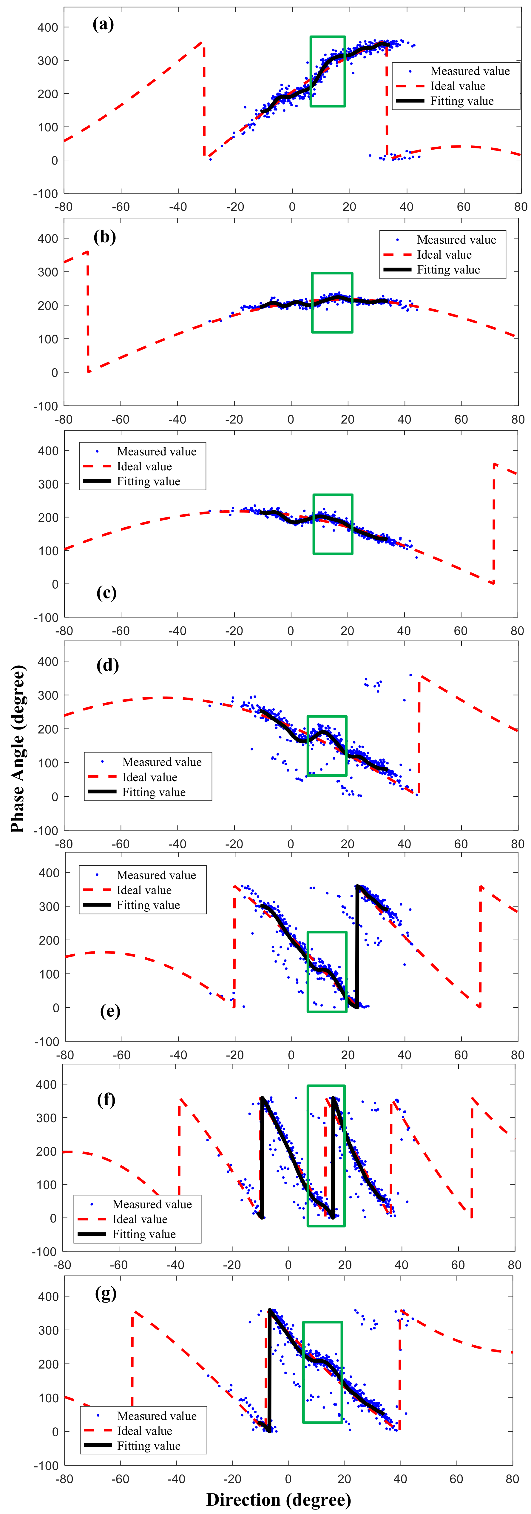
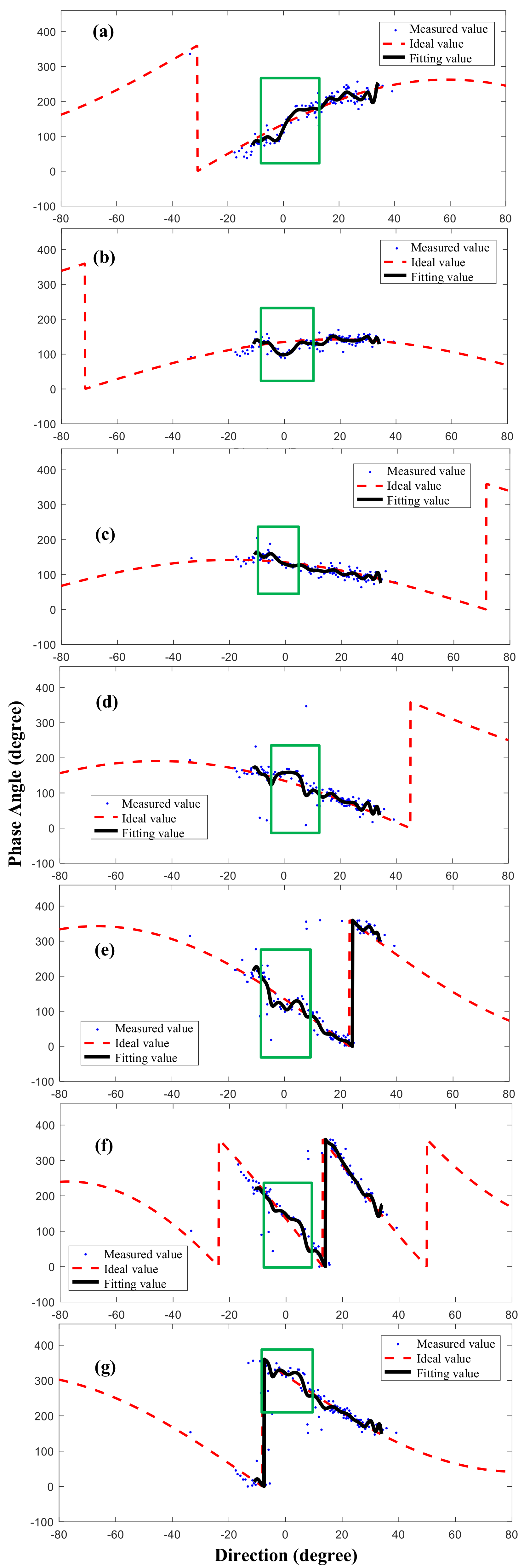
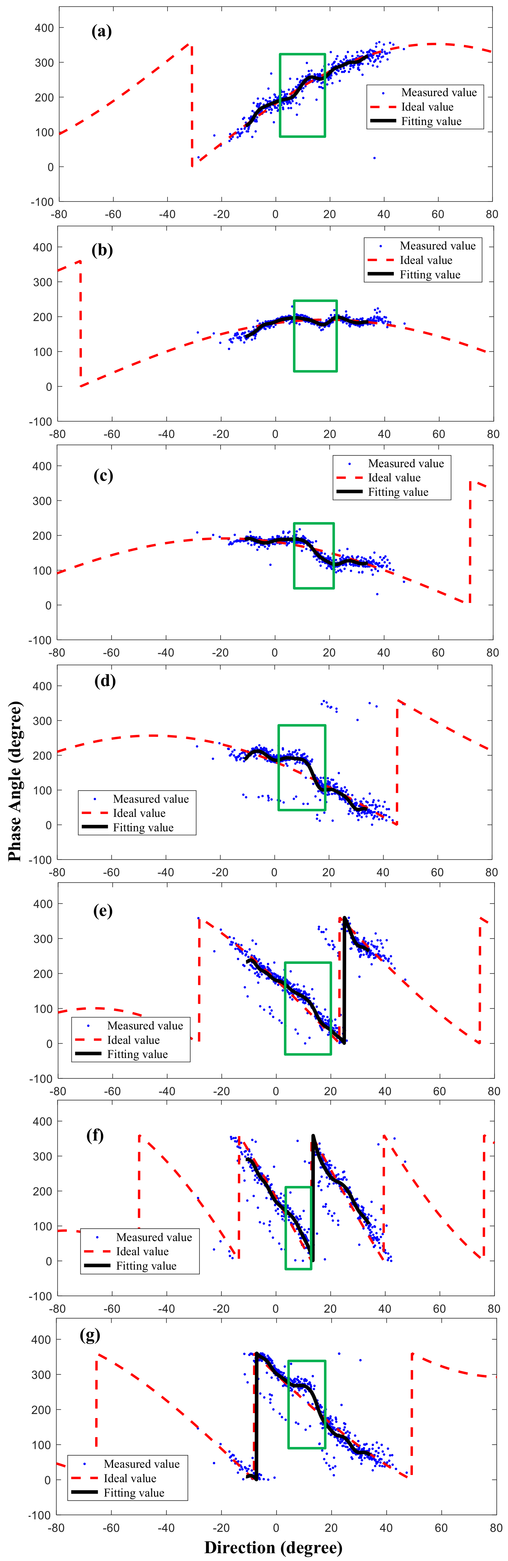
2.3. Array Phase Manifold Estimation

For a known ship echo with a relatively high signal-to-noise ratio (SNR), e.g., 20 dB, the estimate of array phase manifold, which is denoted as $\widehat{B_m\left(\theta \right)}$, can be obtained from receiving signals as:

$$\widehat{B_m\left(\theta \right)}=\frac{z_m\left(t\right)}{z_1\left(t\right)}=\frac{g_m\left(\theta \right)e^{j\left({\varphi }_m\left(\theta \right)+\omega {\tau }_m\right)}s\left(t\right)+n_m\left(t\right)}{g_1\left(\theta \right)e^{j({\varphi }_1\left(\theta \right)+\omega {\tau }_1)}s\left(t\right)+n_1\left(t\right)}.$$

(10)

The phase angle of $\widehat{B_m\left(\theta \right)}$, which is denoted as $\widehat{{\phi }_m\left(\theta \right)}$, can be estimated as

$$\widehat{{\phi }_m\left(\theta \right)}={\varphi }_m\left(\theta \right)-{\varphi }_1\left(\theta \right)+\omega ({\tau }_m-{\tau }_1).$$

(11)

According to (10) and (11), a method for estimating the array phase manifold $\mathit{B}\left(\theta \right)$ while using antenna responses of incoming ship echoes (abbreviated as APM method) is proposed. The steps are as follows:

• Use the MU method to compensate the phase errors of the antenna array.
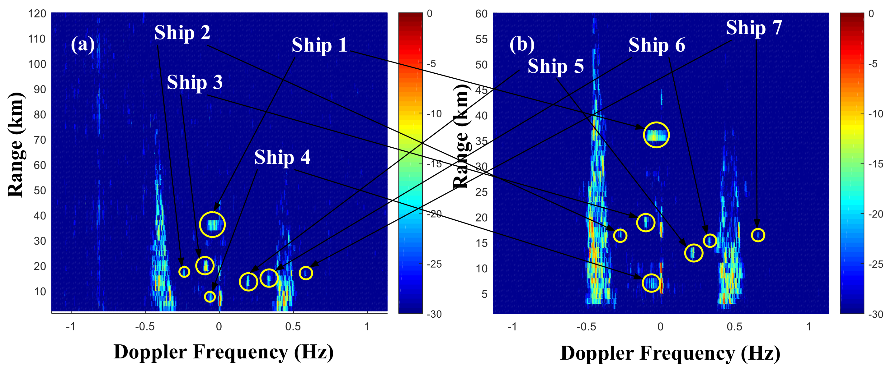
• Detect ships by applying a constant false alarm rate (CFAR)-based method [32] to the range-Doppler spectra.
• Discard the detected ship echoes in the first-order clutter zone. The Doppler frequency of the first-order clutter zone is assumed to be in the band from $-1.3f_B$ to $-0.7f_B$ and from $0.7f_B$ to $1.3f_B$ ($f_B$ denotes the Doppler Bragg frequency).
• Obtain ship information, such as time, range, and radial velocity from both radar and AIS data.
• Determine whether the radar echoes obtained in Step 3 are ship echoes using AIS data.
• Calculate the phase data of the ship echoes by using Equations (10) and (11). From the AIS data the Doppler frequency of the individual ship, $f_{ais}$, can be calculated. If the ship peak exists in the frequency range from $f_{ais}-5\ast \Delta f$ to $f_{ais}+5\ast \Delta f$ ($\Delta f$ denotes the Doppler frequency resolution), the individual ship is matched to the AIS data.
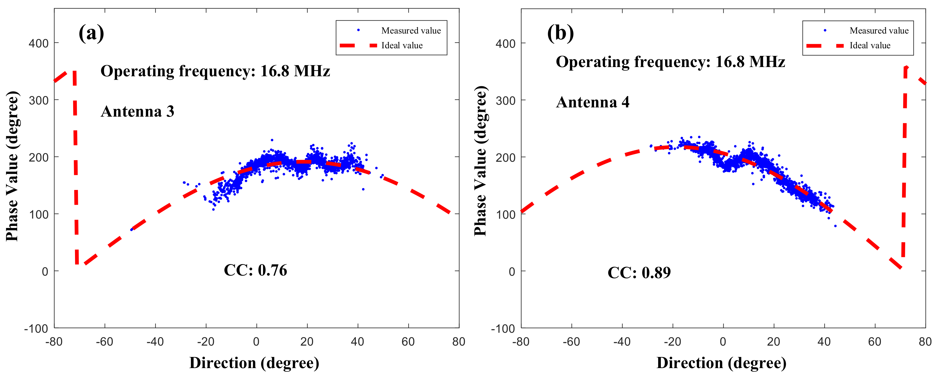
• Apply a least-squares fitting to ship echoes to obtain the phase angle of $\widehat{B_m\left(\theta \right)}$, then the array phase manifold $\widehat{B_m\left(\theta \right)}$ is calculated.

Because the bearing distribution of incoming ship echoes is random, a least-squares fitting method based on a polynomial model is employed to estimate the complex value $\widehat{B_m\left(\theta \right)}$ in Step 7. This polynomial model can be expressed as

$$\mathrm{y}=p\left(1\right)x^b+p\left(2\right)x^{b-1}+...+p\left(b\right)x+p(b+1),$$

(12)

where x denotes the bearing of incoming signal, y represents $\widehat{B_m\left(\theta \right)}$ in (11), and b is the order of the polynomial function ($b=30$ in this work). For a small b (e.g., $4,10,or$ 15), the fitted $\widehat{B_m\left(\theta \right)}$, which is obtained using (12), can not match well with ship echoes. In contrast, for a big b (e.g., 50), it may need more ship echoes. It seems that $b=30$ is appropriate to obtain $\widehat{B_m\left(\theta \right)}$ from hundreds of ship echoes for the MHF radar. It can be seen from the steps that the approach takes few seconds while using a computer and needs accessional AIS antenna and receiver.

2.4. DOA Estimation for Ship Detection and Current Measurement

The MUSIC algorithm is used for HF radar DOA estimation and current measurement. For phase error calibration, the phase error of the received signals should be compensated first (i.e., $\mathit{Z}$ in (3) is obtained). Subsequently, the covariance matrix $\mathit{R}$ of the received signals can be obtained

$$\mathit{R}=E\left[\mathit{Z}{\mathit{Z}}^H\right],$$

(13)

where H denotes the Hermitian transpose operation and E represents the mathematical expectation. The spatial spectrum, $\mathit{P}$, obtained from $\mathit{R}$ in (13) while using the MUSIC algorithm can be expressed by (e.g., see [17])

$$\mathit{P}\left(\theta \right)=\frac{1}{\mathit{A}{\left(\theta \right)}^H{\mathit{E}}_{\mathit{N}}{\mathit{E}}_{\mathit{N}}^H\mathit{A}\left(\theta \right)},$$

(14)

where ${\mathit{E}}_{\mathit{N}}$ represents the noise subspace derived from the eigen-decomposition of the covariance matrix $\mathit{R}$. In contrast, the utility of the measured array phase manifold for the MUSIC algorithm is different. The term $\mathit{A}$ in (14) should be replaced by the measured array phase manifold as:

$$\mathit{P}\left(\theta \right)=\frac{1}{\mathit{B}{\left(\theta \right)}^H{\mathit{E}}_{\mathit{N}}{\mathit{E}}_{\mathit{N}}^H\mathit{B}\left(\theta \right)}.$$

(15)

Eight eigenvalues satisfying $k_1\ge k_2\ge k_3\ge k_4\ge k_5\ge k_6\ge k_7\ge k_8$ are obtained from the eigen-decomposition of the covariance matrix. The biggest gradient of the eigenvalues ($k_1/k_2$, $k_2/k_3$, ..., $k_7/k_8$) is calculated as the boundary between the signal subspace and noise subspace.

3. Radar and Array Manifold Measurement

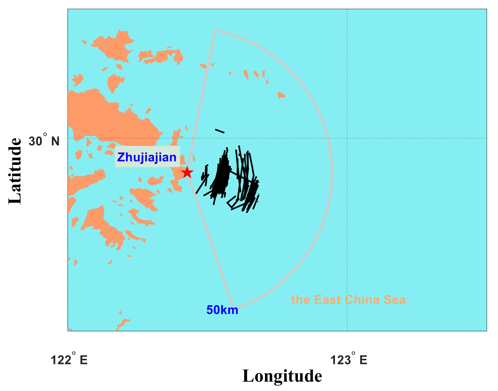
3.1. MHF Radar

The datasets that were selected in this work were collected with a MHF radar installed at Zhujiajian along the coast of the East China Sea from 28 August to 1 September 2009.

Table 1. Capabilities of the MHF Radar System.

Parameter	Value
Operating frequency range (MHz)	7.5–25
Number of operating frequencies	≤4
Transmitter peak power (W)	300
Range cell resolution (km)	1–5
Doppler sampling cycle (s)	0.4–0.6
Measurement cycle (min)	10

provides the details on the radar parameters. The transmitting antennas and receiving antennas are separated. The receiving array consisting of eight monopole antennas requires an occupying area of $54\times 12{\mathrm{m}}^2$, and the positions of the receiving antennas are shown in Figure 2. The steering vector of radar array can be theoretically calculated using the positions of the antennas. During the experiment, the MHF radar operated in a time division multiple sweep mode at 12.5 MHz, 16.8 MHz, and 19.1 MHz, with range resolutions of 5 km, 2 km, and 1 km, respectively. A 512-point fast Fourier transform (FFT) with a 75% overlap is applied to the raw radar data to obtain the Doppler spectra. Every covariance matrix consists of eight snaps. Therefore, 1408 chirps are involved in order to estimate the DOAs while using the MUSIC algorithm.

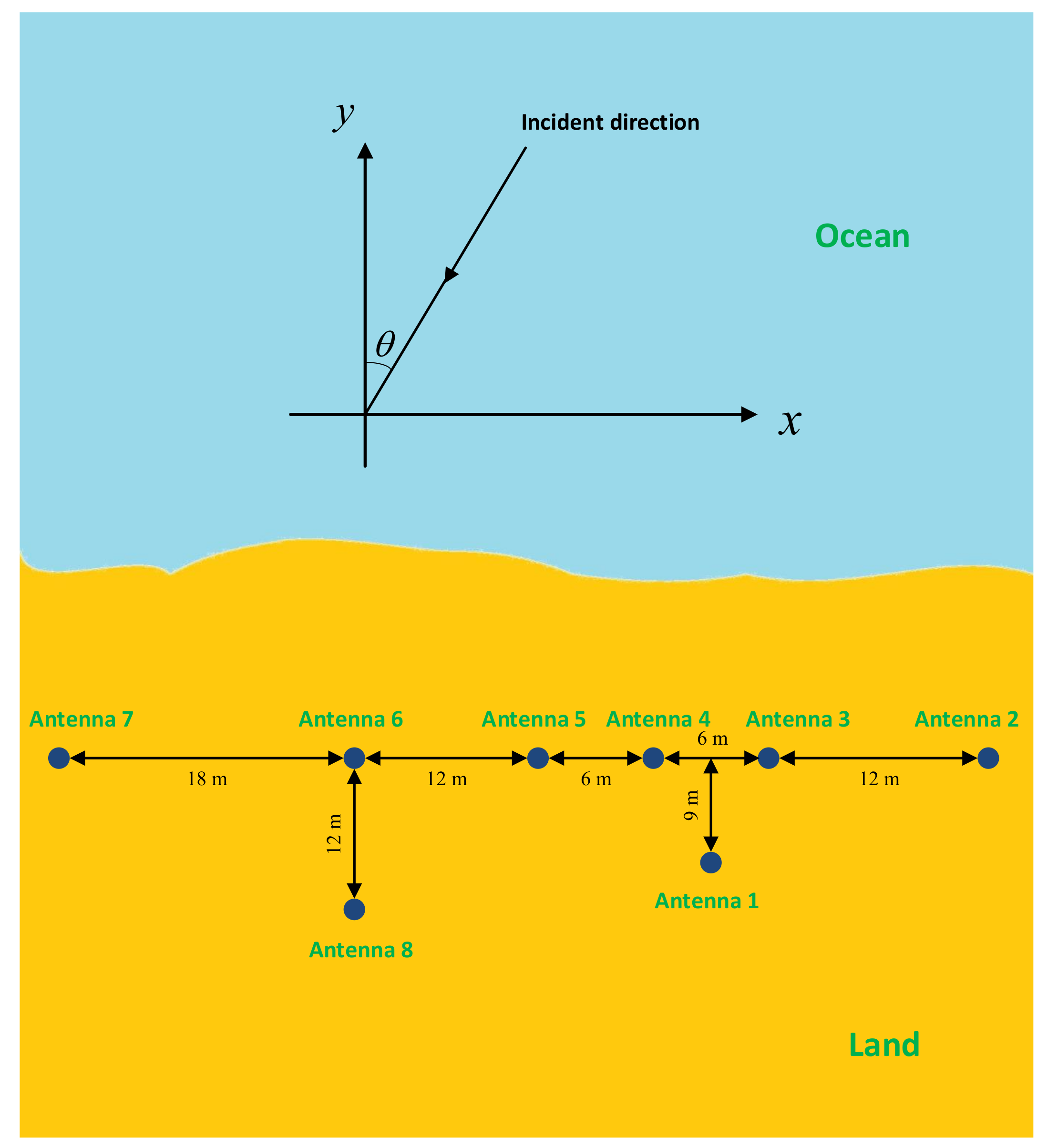
3.2. Array Manifold Measurement

There is a harbor near the Zhujiajian radar site, and lots of ships pass through the radar coverage everyday. Figure 3a,b show two range-Doppler spectra that were collected at 16.8 MHz and 19.1 MHz at 10:40 a.m. on 28 August 2009, respectively. Each range-Doppler spectrum contains seven peaks that are caused by ships. In an attempt to measure the array manifold using ship echoes, an AIS, which is an automatic tracking system that is commonly used on ships and by vessel traffic services (VTS) for identifying and locating vessels, was installed near the radar station during this experiment. The AIS system provided real-time information of ships (e.g., position and speed) within an approximate 100 km radius. In the meantime, the Zhujiajian MHF radar received the echoes of corresponding ships. Therefore, combining AIS and MHF radar data together, ship echoes, as well as the ship locations relative to the radar array, were collected.

The ship echoes outside the first-order clutter zone, which may not be masked in sea clutter, are convenient to identify. A minimum SNR of 20 dB is required for array phase manifold measurement in this study. It can be found that array phase manifold is also a function of radio wavelength. Therefore, the array phase manifold needs to be measured at every radio frequency. Figure 4 shows an example of ships that meet the requirement to measure array phase manifold at 19.1 MHz. The distances between the selected ships and the radar are mostly less than 50 km.

Figure 5 shows the phase angles of the measured array phase manifold at 19.1 MHz. The red dashed lines, which are simulated using (6) from the receiving array configuration of the MHF radar as Figure 2, denote the ideal phase angles of $B_m\left(\theta \right)$ against signal direction $\theta$. The blue dots represent the measured phase angles $\widehat{{\phi }_m}$, which are obtained from ship echoes using Equations (10) and (11). The black lines are acquired by applying a least-squares fitting to blue dots. Consequently, the array phase manifold at operating frequency of 19.1 MHz is obtained using actual phase angles against signal directions relative to antenna boresight from −15 to ${35}^{°}$ (the black lines). Note that phase errors have been compensated in the figure. The fitting values (black solid lines) roughly coincide with theoretical values (red dashed lines). However, in some bearing range (as the green rectangle shown in Figure 4, approximately from 13 to ${20}^{°}$), the fitting values are not in agreement with the theoretical values. This disagreement is caused by the phase distortion of antenna array. In the phase distortion situation, the theoretical values would bring errors to DOA estimations. By the same way, array phase manifolds at operating frequencies of 12.5 MHz and 16.8 MHz are also measured using ship echoes, as shown in Figure 6 and Figure 7. Figure 8a–c show the number of AIS points with ship DOAs. Figure 8d–f show the mean differences between the ideal phase and the fitting phase against direction at 12.5 MHz, 16.8 MHz, and 19.1 MHz, respectively. In the phase distortion range (as the black rectangle shown), the mean differences are larger than those in the other ranges.

4. Results

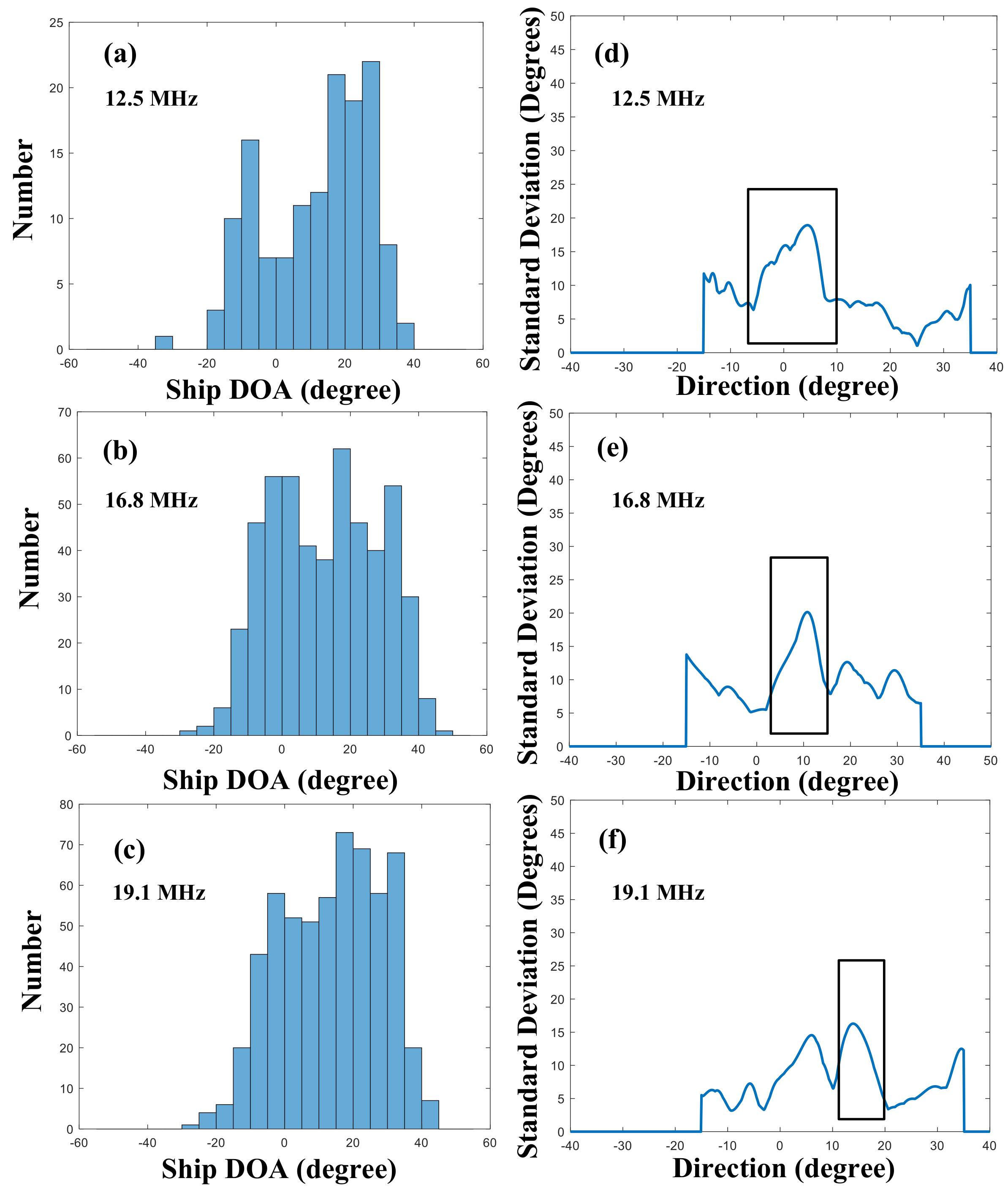
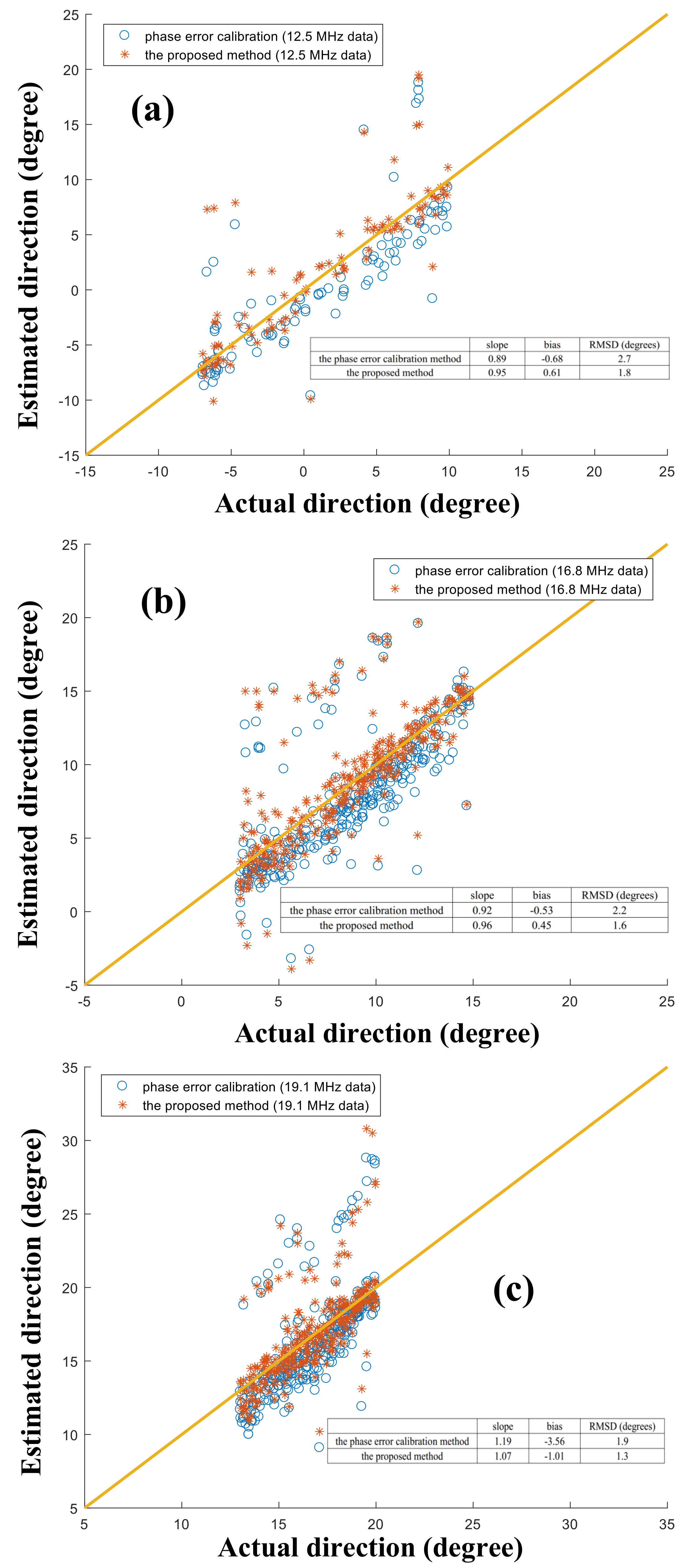
4.1. Ship DOA Estimation

Ship DOAs are estimated from the MHF radar data using the MUSIC algorithm, which is an eigenstructure-based method, in order to evaluate the performance of the proposed calibration method. The ship bearings provided by the AIS are treated as ‘true direction’. As shown in Figure 9, DOA estimation comparisons are made among three data calibration strategies: no calibration, phase error calibration, and array manifold calibration. No calibration means that the radar datasets have not been compensated before DOA estimation. Phase error calibration represents that phase errors of the radar have been compensated using a MU method before DOA estimation [28]. The MU method forms a cost function using the eigenstructure decomposition of single-DOA first-order sea echoes, and the phase errors in array are estimated by minimizing the cost function through an iterative procedure. For phase error calibration, the MU method and the ML approach have already been compared in the previous work [18], and that work indicates that the MU method is better than the ML approach for the MHF radar. Therefore, the MU method is adopted for comparison in this paper. Array manifold calibration means that the array phase manifold has been measured while using the APM method that was introduced in Section 2.3, and ship DOAs are estimated using the method presented in Section 2.4.

The MHF radar operated at 12.5 MHz, 16.8 MHz, and 19.1 MHz from 10:00 a.m. 28 August to 07:30 p.m. 1 September 2009. The array phase manifold measurement is taken using the datasets from 12:00 a.m. 31 August to 07:30 p.m. 1 September 2009, whereas the datasets that were collected from 10:00 a.m. 28 August to 12:00 p.m. 30 August 2009 are selected for comparisons. After combining ship echoes and AIS data, 467, 1638, and 1855 ship echoes are, respectively, used for comparisons for the radar datasets at operating frequencies of 12.5 MHz, 16.8 MHz, and 19.1 MHz. The root mean square deviations (RMSDs) of ship DOA estimation using the no calibration approach at these three operating frequencies are all larger than 18 degrees, as shown in

Table 2. Ship DOA estimation with the Zhujiajian MHF radar using three calibration strategies.

Operating Frequency	Ship Number	RMSD (degrees)
		No Calibration	Phase Error Calibration	The APM Method
12.5 MHz	467	18.3	1.6	1.3
16.8 MHz	1638	22.8	1.8	1.5
19.1 MHz	1855	24.9	1.6	1.4

. In contrast, both calibration strategies using the MU method and the APM method significantly improve the DOA estimation performance compared with the no calibration approach. The results indicate that the APM method is the best among these three strategies with RMSDs around 1.5 degrees at these operating frequencies.

For the 19.1 MHz datasets, significant phase distortion approximately occurs in the bearing range of radar array from 13 to ${20}^{°}$, as shown in Figure 5 and Figure 8f. The datasets at 12.5 MHz and 16.8 MHz have also been tested. In the radar bearing range from $-7$ to ${10}^{°}$ at 12.5 MHz and from 3 to ${15}^{°}$ at 16.8 MHz, the phase distortion is significant. As shown in

Table 3. Ship DOA estimation in the radar bearing range where phase distortion is significant.

Operating Frequency	Ship Number	Bearing Range	RMSD (degrees)
			Phase Error Calibration	The APM Method
12.5 MHz	96	from $-7$ to ${10}^{°}$	2.7	1.8
16.8 MHz	302	from 3 to ${15}^{°}$	2.2	1.6
19.1 MHz	290	from 13 to ${20}^{°}$	1.9	1.3

and Figure 10, in the radar bearing range where the phase distortion is significant, the ship DOA measurement accuracy using the phase error calibration method drops. The APM method shows better performance than the phase error calibration method for the phase distortion cases. The RMSDs are reduced from 2.7 degrees to 1.8 degrees at 12.5 MHz, from 2.2 degrees to 1.6 degrees at 16.8 MHz, and from 1.9 degrees to 1.3 degrees at 19.1 MHz. In the case that phase distortion is significant, the RMSDs have been reduced around $30\%$ while using the APM method compared with the phase error calibration method. The slopes and biases of ship DOA measurements at 12.5 MHz, 16.8 MHz, and 19.1 MHz are also shown in Figure 10. When comparing with the phase error calibration method, the slopes of the ship DOA measurements using the APM method are closer to 1, and the biases are smaller. This also indicates that the APM method is better than the phase error calibration method.

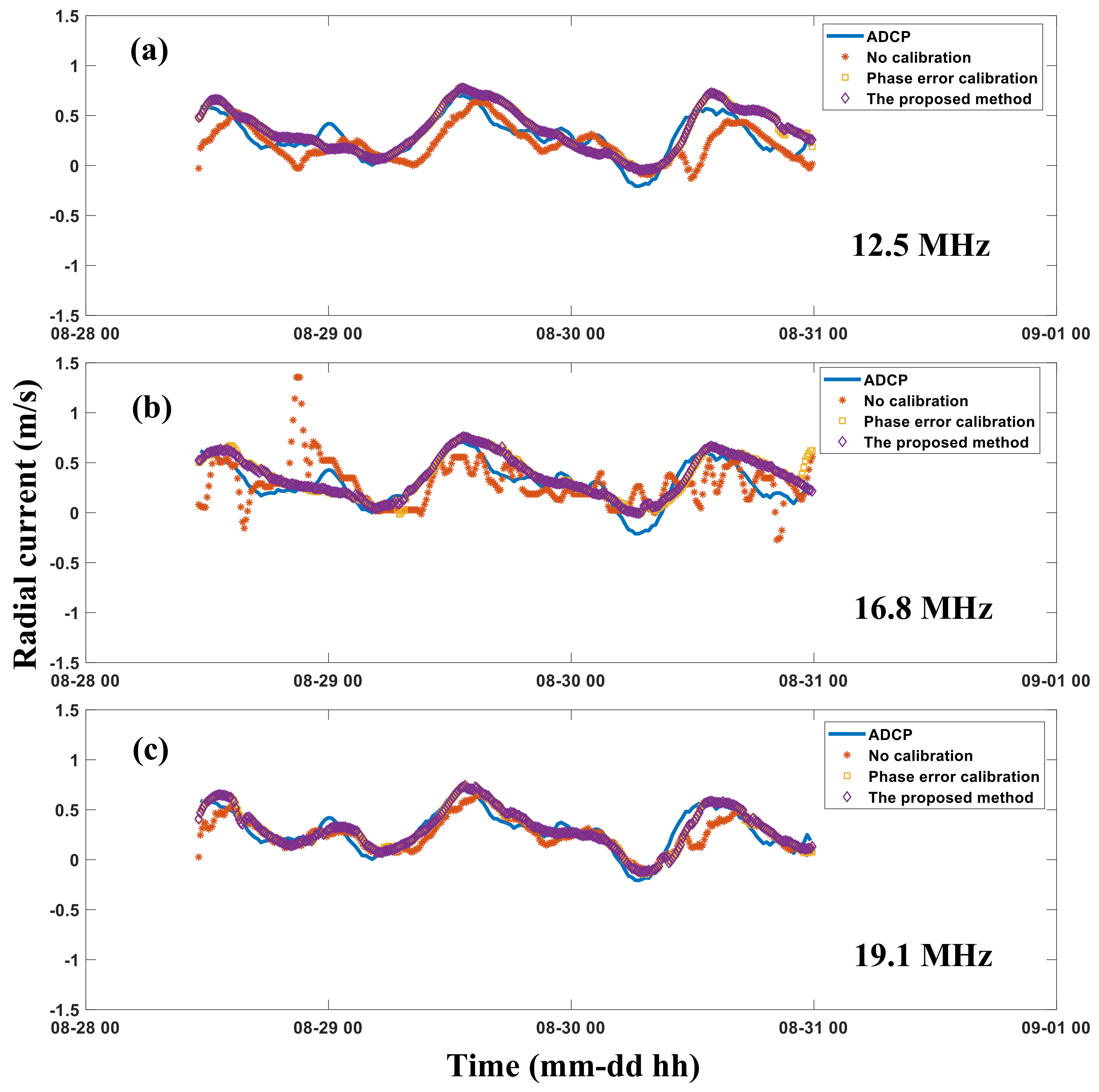
4.2. Current Measurements

The MHF radar was employed to provide current maps over a portion of the East China Sea near Zhejiang Province. Currents in this area are complex, and the radial current $v_R$ obtained from the MHF radar is a function of radar look direction ${\theta }_R$, i.e. $v_R=vcos({\theta }_C-{\theta }_R)$, where v is the current velocity and ${\theta }_C$ denotes the current direction. Consequently, making a comparison of radar-measured radial current against ‘ground-truth’ data is a convincing way to evaluate calibration methods that significantly affect the estimation of radar look direction ${\theta }_R$.

The radial currents obtained from the MHF radar data using three calibration strategies (no calibration, phase error calibration, and array manifold calibration) are compared with Acoustic Doppler Current Profilers (ADCP) current measurements that are considered as ‘ground-truth’ data. A bottom-mounted upward-looking ADCP was deployed at the cell that is 10 km from the radar and $-{10}^{°}$ from the radar boresight. The ADCP provided current vector profiles at depths from approximately 3 m to 20 m at a resolution of 1 m and an interval of 20 min. The ADCP-measured current vectors at the depth of 3 m are converted to radial currents for comparisons.

Radar-derived radial currents are estimated from all eight receiving elements data while using the MUSIC algorithm every 10 minutes. Details on the MHF radar current measurements can be found in [1]. A first-order signal SNR threshold of 10 dB and a MUSIC spectrum SNR threshold of 6 dB are configured for quality control. Figure 11a–c show the radial current comparisons at operating frequencies of 12.5 MHz, 16.8 MHz, and 19.1 MHz, respectively. CCs and RMSDs are reported in

Table 4. Radial current measurements with the Zhujiajian MHF radar using three calibration strategies.

Operating Frequency	No Calibration		Phase Error Calibration		The APM Method
	CC	RMSD (cm/s)	CC	RMSD (cm/s)	CC	RMSD (cm/s)
12.5 MHz	0.65	17.5	0.83	13.1	0.86	12.6
16.8 MHz	0.40	22.4	0.82	13.1	0.86	12.6
19.1 MHz	0.81	12.7	0.91	9.1	0.93	8.4

. When compared with the no calibration approach, both phase error calibration and APM methods significantly improve the current measurement performance. For example, at 16.8 MHz, the current measurements without array calibration are poor with a CC of 0.40 and a RMSD of 22.4 cm/s, whereas current measurements obtained by using the phase error calibration and the APM methods are consistent with ADCP-measured currents, with CCs of 0.82 and 0.86, respectively. The CCs and RMSDs indicate that the measurements obtained using the APM method are better than those using the phase error calibration method. Additionally, the comparisons at operating frequencies of 12.5 MHz and 19.1 MHz indicate that the APM method is the best.

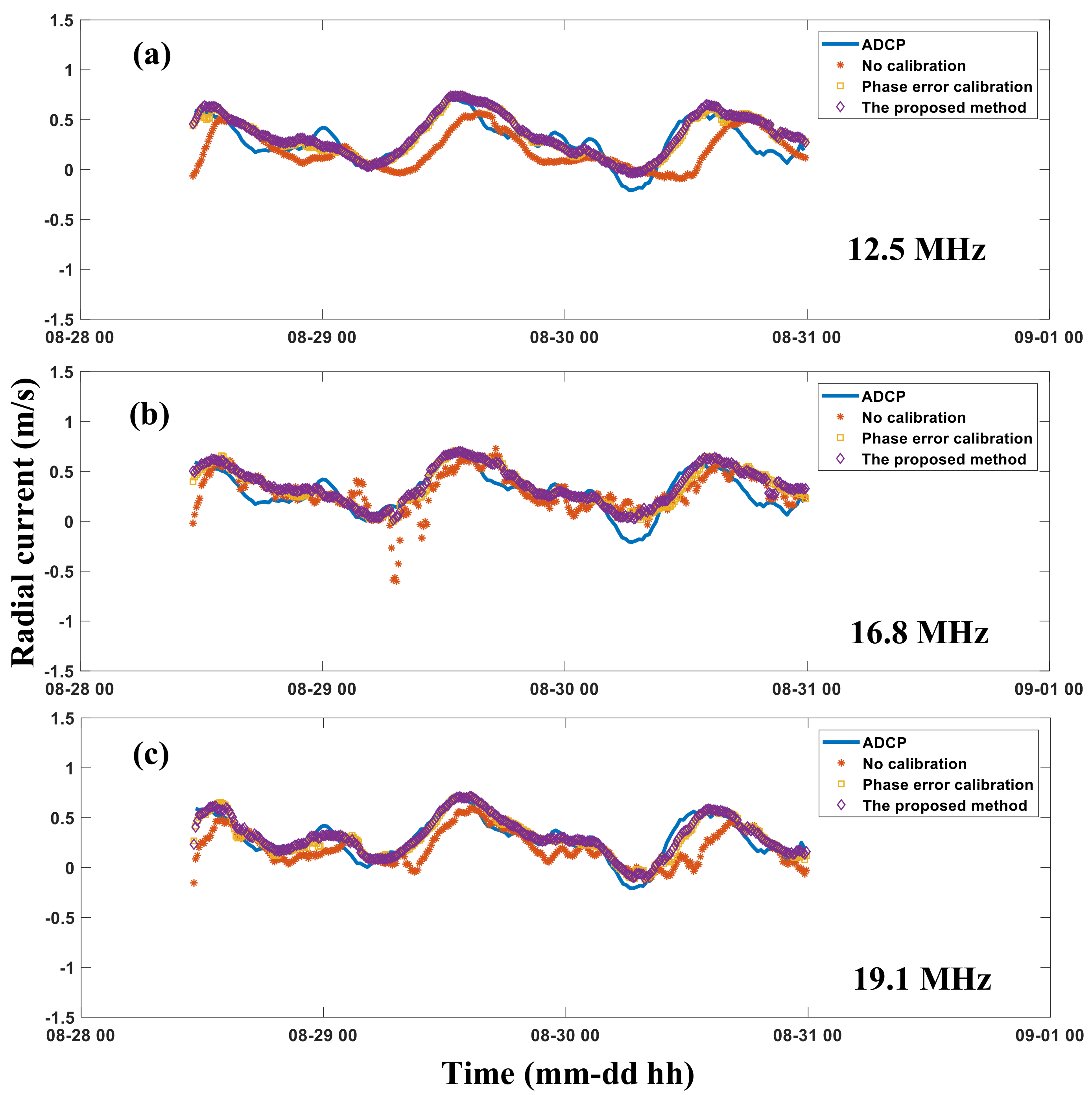
4.3. Current Measurements Using Four Receiving Elements

For a special antenna configuration, radial currents are obtained from four-element MHF radar datasets. The four receiving elements are antenna 2, antenna 3, antenna 4, and antenna 5, which are deployed as the configuration that is shown in Figure 2. The experiment is conducted in this way, because the four-element configuration has been employed in some phase-mode direction-finding radars, e.g., the compact WERA system that was developed by the Heltz company and the High Frequency Doppler Radio scatterometers (HFDR) in direction-finding mode developed by University of Hawaii. Radial currents which are obtained from the MHF radar datasets at the location of ADCP using three calibration strategies are compared with ADCP measurements. Figure 12a–c show the results at operating frequencies of 12.5 MHz, 16.8 MHz, and 19.1 MHz, respectively. CCs and RMSDs are listed in

Table 5. Radial current measurements with the Zhujiajian MHF radar using three calibration strategies. Only four-element datasets are involved in the MHF radar radial current measurements

Operating Frequency	No Calibration		Phase Error Calibration		The APM Method
	CC	RMSD (cm/s)	CC	RMSD (cm/s)	CC	RMSD (cm/s)
12.5 MHz	0.43	22.8	0.82	14.3	0.85	13.1
16.8 MHz	0.57	18.7	0.82	14.6	0.86	13.1
19.1 MHz	0.63	18.6	0.89	9.2	0.92	8.9

. The agreement using the APM method is the best with CCs of 0.85, 0.86, and 0.92, at operating frequencies of 12.5 MHz, 16.8 MHz, and 19.1 MHz, respectively, while the worst result is obtained using the no calibration approach with CCs being less than 0.65 at these three operating frequencies.

5. Discussion

HF radar current measurement and target detection performance is associated with DOA estimation capability, which strongly depends on the accuracy of array manifold. Both the proposed calibration technique (APM method) and traditional phase error calibration method (MU method) show significant improvements on HF radar DOA estimation and current measurement comparing with the no calibration strategy. In the case that phase distortion is significant, the RMSDs have been reduced while using the APM method as compared with the MU method.

For current comparison, the ADCP was deployed at the cell, which is $-{10}^{°}$ from the radar boresight. At this bearing the phase distortions of the radar at these three operating frequencies are not significant (see Table 3). At the bearing of $-{10}^{°}$, the steering vector for the MU method $\mathit{A}(-{10}^{°})$ and the steering vector for the APM method $\mathit{B}(-{10}^{°})$ are approximately the same. As a consequence, the DOA performances at the bearing of $-{10}^{°}$ using the APM method and the phase error method are nearly the same. This is why the APM method slightly, but not significantly, improves the current measurement performance compared with the MU method for these datasets.

Another interesting work is that the APM method has been applied to four-element HF radar datasets. As reported in Table 5, the current measurements that were obtained from the four-element HF radar datasets using the APM method are as good as those obtained from eight-element MHF radar datasets using the MU method. This is extremely useful for compact HF radars, since they are more convenient than large array radar to deploy.

6. Conclusions

The receiving array signal model for a phased-array HF radar has been investigated and modified. Phase distortions have been observed in the MHF radar receiving elements. The APM method based on measuring array manifold HF radar ship echoes as well as AIS data has been proposed. The performance of the APM method has been compared with the no calibration strategy and the phase error calibration method.The DOA estimations and current measurements using the MUSIC algorithm show a reasonable improvement after taking the phase distortion into consideration and using the APM method.

Array calibration is critical for HF surface wave radar applications, and it can significantly improve azimuth estimation performance as well as current measurements. The phase error calibration, which has been studied in the past few decades, is not sufficient for the MHF radar in the phase distortion situation. The APM method provides a feasible way to measure the array manifold and calibrate the array distortion. This method will be validated in other radar sites in the future.

References

1. Zhao, C.; Chen, Z.; Zeng, G.; Zhang, L.; Xie, F. Evaluating radial current measurement of multifrequency HF radar with multidepth ADCP data during a small storm. J. Atmos. Ocean. Technol. 2015, 32, 1071–1087. [Google Scholar] [CrossRef]
2. Chen, Z.; Zhao, C.; Jiang, Y.; Hu, W. Wave measurements with multi-frequency HF radar in the East China Sea. J. Electromagn. Waves Appl. 2011, 25, 1031–1043. [Google Scholar] [CrossRef]
3. Zhao, C.; Chen, Z.; He, C.; Xie, F.; Chen, X. A Hybrid Beam-Forming and Direction-Finding Method for Wind Direction Sensing Based on HF Radar. IEEE Trans. Geosci. Remote Sens. 2018, 56, 6622–6629. [Google Scholar] [CrossRef]
4. Grosdidier, S.; Baussard, A.; Khenchaf, A. HFSW radar model: Simulation and measurement. IEEE Trans. Geosci. Remote Sens. 2010, 48, 3539–3549. [Google Scholar] [CrossRef]
5. Anderson, S.J. Optimizing HF Radar Siting for surveillance and remote sensing in the strait of Malacca. IEEE Trans. Geosci. Remote Sens. 2013, 51, 1805–1816. [Google Scholar] [CrossRef]
6. Le Caillec, J.M.; Mandridake, L. Influence of the waveform on propagation and sea radar cross section of HF radar signals. IEEE Trans. Antennas Propag. 2014, 62, 2721–2735. [Google Scholar]
7. Chavanne, C.; Janeković, I.; Flament, P.; Poulain, P.M.; Kuzmić, M.; Gurgel, K.W. Tidal currents in the northwestern Adriatic: High-frequency radio observations and numerical model predictions. J. Geophys. Res. Ocean. 2007, 112. [Google Scholar] [CrossRef] [Green Version]
8. Liu, Y.; Weisberg, R.H.; Merz, C.R.; Lichtenwalner, S.; Kirkpatrick, G.J. HF radar performance in a low-energy environment: CODAR SeaSonde experience on the West Florida Shelf. J. Atmos. Ocean. Technol. 2010, 27, 1689–1710. [Google Scholar] [CrossRef]
9. Paduan, J.D.; Washburn, L. High-frequency radar observations of ocean surface currents. Annu. Rev. Mar. Sci. 2013, 5, 115–136. [Google Scholar] [CrossRef] [Green Version]
10. Dzvonkovskaya, A.; Rohling, H. HF radar performance analysis based on AIS ship information. In Proceedings of the 2010 IEEE Radar Conference, Washington DC, USA, 10–14 May 2010; pp. 1239–1244. [Google Scholar]
11. Fernandez, D.M.; Vesecky, J.F.; Barrick, D.; Teague, C.C.; Plume, M.; Whelan, C. Detection of ships with multi-frequency and CODAR SeaSonde HF radar systems. Can. J. Remote Sens. 2001, 27, 277–290. [Google Scholar] [CrossRef]
12. Wyatt, L.R.; Mantovanelli, A.; Heron, M.L.; Roughan, M.; Steinberg, C.R. Assessment of surface currents measured with high-frequency phased-array radars in two regions of complex circulation. IEEE J. Ocean. Eng. 2018, 43, 484–505. [Google Scholar] [CrossRef] [Green Version]
13. Kamli, E.; Chavanne, C.; Dumont, D. Experimental assessment of the performance of high-frequency CODAR and WERA radars to measure ocean currents in partially ice-covered waters. J. Atmos. Ocean. Technol. 2016, 33, 539–550. [Google Scholar] [CrossRef]
14. Zhao, C.; Chen, Z.; He, C.; Xie, F.; Chen, X.; Mou, C. Validation of Sensing Ocean Surface Currents Using Multi-Frequency HF Radar Based on a Circular Receiving Array. Remote Sens. 2018, 10, 184. [Google Scholar] [CrossRef] [Green Version]
15. Gurgel, K.W.; Antonischki, G.; Essen, H.H.; Schlick, T. Wellen Radar (WERA): A new ground-wave HF radar for ocean remote sensing. Coast. Eng. 1999, 37, 219–234. [Google Scholar] [CrossRef]
16. Zhao, C.; Chen, Z.; Jiang, Y.; Fan, L.; Zeng, G. Exploration and validation of wave-height measurement using multifrequency HF radar. J. Atmos. Ocean. Technol. 2013, 30, 2189–2202. [Google Scholar]
17. Kirincich, A.; Emery, B.; Washburn, L.; Flament, P. Improving Surface Current Resolution Using Direction Finding Algorithms for Multiantenna High-Frequency Radars. J. Atmos. Ocean. Technol. 2019, 36, 1997–2014. [Google Scholar] [CrossRef]
18. Zhao, C.; Chen, Z.; Zeng, G.; Zhang, L. Evaluating two array autocalibration methods with multifrequency HF radar current measurements. J. Atmos. Ocean. Technol. 2015, 32, 1088–1097. [Google Scholar] [CrossRef]
19. Schmid, C.M.; Schuster, S.; Feger, R.; Stelzer, A. On the effects of calibration errors and mutual coupling on the beam pattern of an antenna array. IEEE Trans. Antennas Propag. 2013, 61, 4063–4072. [Google Scholar] [CrossRef]
20. Tian, Y.; Wen, B.; Tan, J.; Li, Z. Study on pattern distortion and DOA estimation performance of crossed-loop/monopole antenna in HF radar. IEEE Trans. Antennas Propag. 2017, 65, 6095–6106. [Google Scholar] [CrossRef]
21. De Paolo, T.; Terrill, E. Skill assessment of resolving ocean surface current structure using compact-antenna-style HF radar and the MUSIC direction-finding algorithm. J. Atmos. Ocean. Technol. 2007, 24, 1277–1300. [Google Scholar] [CrossRef]
22. Emery, B.M.; Washburn, L.; Whelan, C.; Barrick, D.; Harlan, J. Measuring antenna patterns for ocean surface current HF radars with ships of opportunity. J. Atmos. Ocean. Technol. 2014, 31, 1564–1582. [Google Scholar] [CrossRef]
23. Weiss, A.J.; Friedlander, B. Eigenstructure methods for direction finding with sensor gain and phase uncertainties. Circuits Syst. Signal Process. 1990, 9, 271–300. [Google Scholar] [CrossRef]
24. Fabrizio, G.; Gray, D.; Turley, M. Using sources of opportunity to compensate for receiver mismatch in HF arrays. IEEE Trans. Aerosp. Electron. Syst. 2001, 37, 310–316. [Google Scholar] [CrossRef] [Green Version]
25. Xiongbin, W.; Feng, C.; Zijie, Y.; Hengyu, K. Broad beam HFSWR array calibration using sea echoes. In Proceedings of the International Conference on Radar, CIE’06, Shanghai, China, 16–19 October 2006; pp. 1–3. [Google Scholar]
26. Fernandez, D.M.; Vesecky, J.F.; Teague, C. Phase corrections of small-loop HF radar system receive arrays with ships of opportunity. IEEE J. Ocean. Eng. 2006, 31, 919–921. [Google Scholar] [CrossRef]
27. Flores-Vidal, X.; Flament, P.; Durazo, R.; Chavanne, C.; Gurgel, K.W. High-frequency radars: Beamforming calibrations using ships as reflectors. J. Atmos. Ocean. Technol. 2013, 30, 638–648. [Google Scholar] [CrossRef]
28. Chen, Z.; Zeng, G.; Zhao, C.; Zhang, L. A Phase Error Estimation Method for Broad Beam High-Frequency Radar. IEEE Geosci. Remote Sens. Lett. 2015, 12, 1526–1530. [Google Scholar] [CrossRef]
29. Byun, G.; Choo, H. A Novel Approach to Array Manifold Calibration Using Single-Direction Information for Accurate Direction-of-Arrival Estimation. IEEE Trans. Antennas Propag. 2017, 65, 4952–4957. [Google Scholar] [CrossRef]
30. Pralon, M.G.; Del Galdo, G.; Landmann, M.; Hein, M.A.; Thomä, R.S. Suitability of Compact Antenna Arrays for Direction-of-Arrival Estimation. IEEE Trans. Antennas Propag. 2017, 65, 7244–7256. [Google Scholar] [CrossRef]
31. Chen, Z.; Zhang, L.; Zhao, C.; Li, J. Calibration and Evaluation of a Circular Antenna Array for HF Radar Based on AIS Information. IEEE Geosci. Remote. Sens. Lett. 2020, 17, 988–992. [Google Scholar] [CrossRef]
32. Maresca, S.; Braca, P.; Horstmann, J.; Grasso, R. Maritime surveillance using multiple high-frequency surface-wave radars. IEEE Trans. Geosci. Remote Sens. 2014, 52, 5056–5071. [Google Scholar] [CrossRef]
Figure 1. An example of ideal and measured phase values of A m obtained by the MHF radar at 16.8 MHz for different antenna elements. The phase values are measured from ship echoes. (a) Antenna 3; (b) Antenna 4.
Remotesensing 12 02761 g001
Figure 2. The setup of receiving antennas of multi-frequency HF (MHF) radar. The blue dots represent the positions of eight antennas.
Remotesensing 12 02761 g002
Figure 3. Two range-Doppler spectra collected using the Zhujiajian MHF radar at 10:40 a.m. on 28 August 2009. Seven ships are observed in both range-Doppler spectra. (a) 16.8 MHz; (b) 19.1 MHz.
Remotesensing 12 02761 g003
Figure 4. Ships that are used for array phase manifold measurement at 19.1 MHz. Black lines in the map denote the AIS-ship tracks.
Remotesensing 12 02761 g004
Figure 5. Array phase value measurements at 19.1 MHz. (a) Antenna 2; (b) Antenna 3; (c) Antenna 4; (d) Antenna 5; (e) Antenna 6; (f) Antenna 7; and, (g) Antenna 8.
Remotesensing 12 02761 g005
Figure 6. Array phase value measurements at 12.5 MHz. (a) Antenna 2; (b) Antenna 3; (c) Antenna 4; (d) Antenna 5; (e) Antenna 6; (f) Antenna 7; and, (g) Antenna 8.
Remotesensing 12 02761 g006
Figure 7. Array phase value measurements at 16.8 MHz. (a) Antenna 2; (b) Antenna 3; (c) Antenna 4; (d) Antenna 5; (e) Antenna 6; (f) Antenna 7; (g) Antenna 8.
Remotesensing 12 02761 g007
Figure 8. The measure of the number of AIS points with ship DOA: (a) 12.5 MHz; (b) 16.8 MHz; (c) 19.1 MHz. The mean differences between the ideal phase and the fitting phase against direction at: (d) 12.5 MHz; (e) 16.8 MHz; and, (f) 19.1 MHz.
Remotesensing 12 02761 g008
Figure 9. Scatter plot of the ship direction estimation using three data calibration strategies: no calibration, phase error calibration, and array manifold calibration. (a) 12.5 MHz; (b) 16.8 MHz; and, (c) 19.1 MHz.
Remotesensing 12 02761 g009
Figure 10. Scatter plot of the ship direction estimation using the phase error calibration method and the proposed method in the phase distortion case. (a) 12.5 MHz; (b) 16.8 MHz; and, (c) 19.1 MHz.
Remotesensing 12 02761 g010
Figure 11. Comparisons between the MHF radar-derived radial currents and ADCP data. (a) 12.5 MHz; (b) 16.8 MHz; (c) 19.1 MHz.
Remotesensing 12 02761 g011
Figure 12. Comparisons between the MHF radar-derived radial currents and ADCP data. Only four-element datasets are involved in the MHF radar radial current measurements. (a) 12.5 MHz; (b) 16.8 MHz; and, (c) 19.1 MHz.
Remotesensing 12 02761 g012