Climatology Characteristics of Ionospheric Irregularities Described with GNSS ROTI

Abstract

At equatorial and high latitudes, the intense ionospheric irregularities and plasma density gradients can seriously affect the performances of radio communication and satellite-based navigation systems; that represents a challenging topic for the scientific and engineering communities and operational use of communication and navigation services. The GNSS-based ROTI (rate of TEC index) is one of the most widely used indices to monitor the occurrence and intensity of ionospheric irregularities. In this paper, we examined the long-term performance of the ROTI in terms of finding the climatological characteristics of TEC fluctuations. We considered the different scale temporal signatures and checked the general sensitivity to the solar and geomagnetic activity. We retrieved and analyzed long-term time-series of ROTI values for two chains of GNSS stations located in European and North-American regions. This analysis covers three full years of the 24th solar cycle, which represent different levels of solar activity and include periods of intense geomagnetic storms. The ionospheric irregularities’ geographical distribution, as derived from ROTI, shows a reasonable consistency to be found within the poleward/equatorward boundaries of the auroral oval specified by empirical models. During magnetic midnight and quiet-time conditions, the equatorward boundary of the ROTI-derived ionospheric irregularity zone was observed at 65–70${}^{°}$ of north magnetic latitude, while for local noon conditions this boundary was more poleward at 75–85 magnetic latitude. The ionospheric irregularities of low-to-moderate intensity were found to occur within the auroral oval at all levels of geomagnetic activity and seasons. At moderate and high levels of solar activity, the intensities of ionospheric irregularities are larger during local winter conditions than for the local summer and polar day conditions. We found that ROTI displays a selective latitudinal sensitivity to the auroral electrojet activity—the strongest dependence (correlation R > 0.6–0.8) was observed within a narrow latitudinal range of 55–70${}^{°}$N magnetic latitude, which corresponded to a band of the largest ROTI values within the auroral oval zone expanded equatorward during geomagnetic disturbances.

1. Introduction

Apart from its primary operational objective, the Global Navigation Satellite System (GNSS) has become one of the most important tools in ionospheric research. The greatest advantages over traditional techniques (such as radar/ionosonde and in situ plasma density measurements) are the global coverage and continuous, permanent availability [1,2,3,4]. Though GNSS signal frequencies have been chosen within the ionospheric disturbances resistant L–band, steeply and rapidly moving plasma density gradients may cause scintillations of the signals phase and intensity [5,6].

The problem of ionospheric plasma density irregularities is very complex, as it depends on a whole range of drivers—from the typical diurnal and seasonal ionization variation to the space weather induced events. Plasma density irregularities in auroral and subauroral latitudes are mainly caused by the auroral particle precipitation and high-speed plasma convection [7,8]. The scale of the processes—and thus the irregularities—can be substantially enlarged during geomagnetic storms and substorms [9,10].

Several ionospheric fluctuations models have already been developed [11,12]; however, most of them focus on weak scintillations in the radio signals. Strong ionospheric irregularities may cause serious signal degradation and harmfully impact precise positioning [13]. Satellite navigation is based on the observations from satellites located in various parts of the sky above the receiver—a proper geometry can provide a higher accuracy [14]. Strong scintillations of the received satellite signals may cause the loss-of-lock and in the worst scenarios affect the overall constellation geometry observed, resulting in a serious degradation of performance or full loss of navigation. Thus, development of the ionospheric fluctuations models is crucial for the GNSS users sector as well.

Additionally, many scientific users are interested in the information about the ionosphere rapid dynamics. Nowadays many facilities for radio astronomy operate on low radio frequencies (below 1 GHz and down to even ionospheric critical plasma frequency). Rapid changes in ionospheric plasma density can significantly affect the performances of such instruments as the Low Frequency Array (LOFAR)—a European radio interferometer operating on a frequency range of 20–240 MHz [15]. Such sensitive instruments as LOFAR provide, also, some possibilities of ionospheric irregularity observations [16].

One of the most commonly used scintillation indices is S4, which directly describes fluctuation-caused variations in the signal amplitude; however, it requires dedicated GNSS receivers. It is possible to obtain phase fluctuations using data from standard geodetic GNSS receivers in various worldwide permanent networks. One of the phase fluctuation measures is the rate of total electron content changes index (ROTI). ROTI is proven to have a direct correlation with radio wave scintillations [17]. Another data product describing phase fluctuation activity using GNSS ROTI measurements is being developed, and since 2018 it has been freely accessible as an International GNSS Service (IGS) ROTI map product [18,19]. For many years, ROTI has been successfully utilized for ionospheric irregularity studies at sub-auroral [3,20,21,22] and equatorial [23,24,25,26,27] latitudes. Most often, a detailed ROTI analysis is performed for particular events or case-studies, such as severe geomagnetic storms. In this work, however, we aimed to study extensively the long-term climatology of the ROTI behavior during different periods and conditions. We found some ROTI characteristics during quiet time; disturbed geomagnetic conditions signatures; and solar activity, seasonal, and diurnal dependencies. Better understanding of the ROTI climatological performance would be an important step towards better modeling of the TEC fluctuations’ occurrence.

In this paper, we present a long-term analysis of ionospheric irregularities based on GNSS ROTI observations to evaluate ROTI capabilities and find the climatological characteristics for the morphology and variability of the ionospheric plasma density irregularity phenomenon at middle and high latitudes depending on diurnal and seasonal cycles, and on geomagnetic activity.

2. Materials and Methods

Today, one of the most commonly-used GNSS-based parameters characterizing the ionospheric plasma density is the total electron content (TEC). In its most basic form (denoted as slant TEC-STEC), it describes the total quantity of free electrons in the ionosphere along the satellite-receiver’s line-of-sight (LOS):

$$STEC=\int n_e\left(s\right)ds$$

(1)

where $n_e$ stands for the number of electrons and s for the path of signal along the LoS. TEC is described in TEC units, denoted as TECU, and equal to ${10}^{16}$ el ∗ m${}^{-2}$.

STEC integrates contributions from all electrons along the LOS through the whole ionospheric layer. There are several approaches describing the TEC distribution within the ionospheric layer. The most common, also used in this study, uses the thin single-layer model, which accumulates the TEC value to a single point (ionospheric pierce point—IPP) on a sphere of unit width fixed to a certain altitude representing the whole layer. In this work, we use 350 km altitude of the ionospheric layer, and an approximation of the free electron maximum density height.

With dual-frequency GNSS receivers, the relative STEC can be directly estimated using a geometry-free combination of GNSS observables [28,29]:

$$STE{C}_i=(\frac{L1}{f_1}-\frac{L2}{f_2})\ast \frac{f_1^2\ast f_2^2}{f_1^2-f_2^2}\ast \frac{c}{K}$$

(2)

where L1 and L2 are carrier phase observations performed on frequencies f1 and f2 for the GPS equal f1 = 1525.42 MHz and f2 = 1227.60 MHz; c is the speed of light in the vacuum; and K is a constant factor equal to 40.3.

Ionospheric irregularities could be described by the fluctuations of the GNSS signals corresponding to the rapid changes in TEC. Rate of TEC described by Pi [1] is a simple time derivative of the TEC calculated along the single, continuous GNSS satellite passing arc:

$$ROT=\frac{TE{C}_{i+1}-TE{C}_i}{t_{i+1}-t_i}$$

(3)

ROT is then a difference of observed nominal slant TEC values in the interval equal to the chosen time unit equal to one minute. ROT is measured in TECU/min. ROT denotes directly the fluctuations of the signal caused by the ionospheric structures. ROT index (ROTI) calculated as a standard deviation of nominal ROT values (Equation (4)) can be used to describe the occurrence of irregularities in the ionospheric plasma density.

$$ROTI=\sqrt{\langle RO{T}^2\rangle -{\langle ROT\rangle }^2}$$

(4)

In this study, we calculated ROTI using a running window for 5-min sets of ROT observations. Then, we calculated hourly and daily average ROTI values within cells of 2 degrees in latitude and 2 degrees in longitude—although the daily averages smooth out some peaks in ROTI values, they can be still treated as reasonable measures of the general irregularity occurrence, as the ROTI median value depends on the observation sampling rate rather than the calculation interval [30]. During calculations, we also split the obtained daily values into local day-time and nighttime averages, with day set as 6:00 a.m.–6:00 p.m. local time (LT) and night as 6:00 p.m.–6:00 a.m. LT. To avoid the multipath effect distortion on the ROTI values, we applied a 30 degree elevation angle cutoff mask.

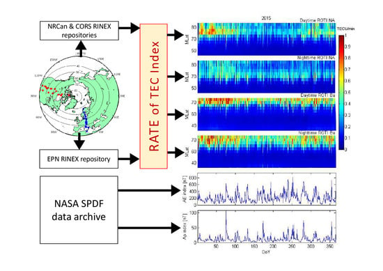
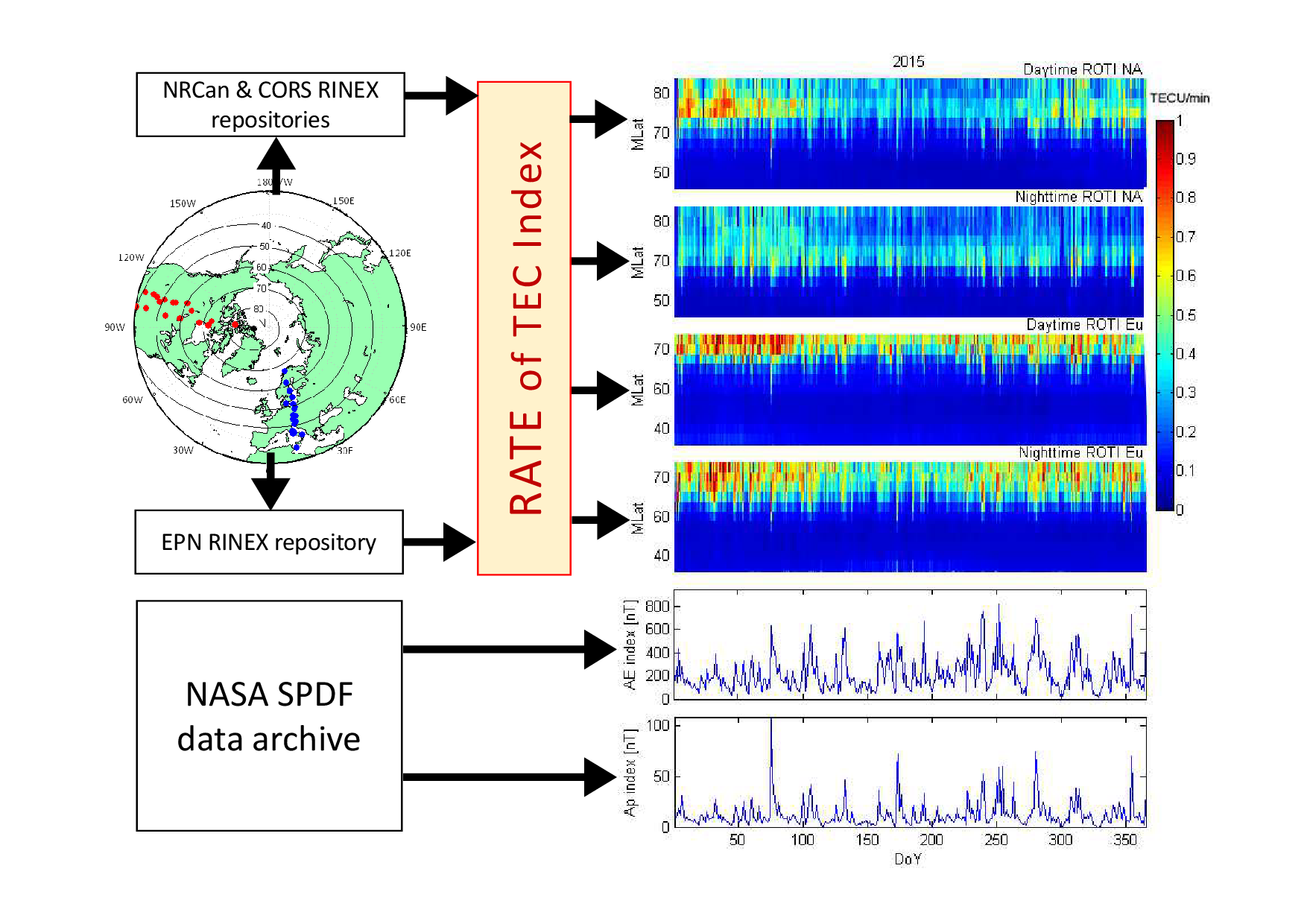
We collected the raw RINEX (receiver independent exchange system) data with a standard 30-s resolution from GNSS permanent stations distributed along two selected meridians, namely, 15${}^{°}$E and 100${}^{°}$W, to illustrate the ionospheric irregularity occurrence in two zones: Europe and North America. 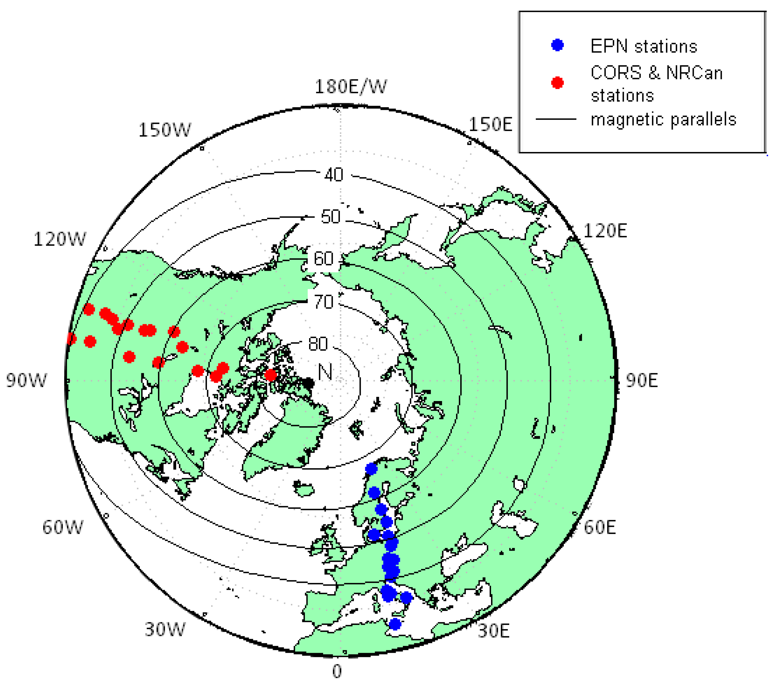Selected chains of GNSS stations belonging to the EUREF Permanent Network (EPN), Continuously Operating Reference Stations (CORS), and Natural Resources Canada (NRCan) properly cover the latitudinal range between ∼30${}^{°}$N and ∼80${}^{°}$N (Figure 1). The collected dataset includes observations over three selected years: 2013, 2015, and 2017, representing high, moderate, and low solar activity periods, respectively. Figure 2 shows the monthly averaged sunspot number for the whole 24th solar cycle and three selected time intervals. Such an approach allows one to analyze different time scales and different aspects—the diurnal, seasonal, and annual variations of the ionospheric fluctuations, and to examine relationships between geomagnetic activity and latitudinal extent of the auroral irregularity occurrence.

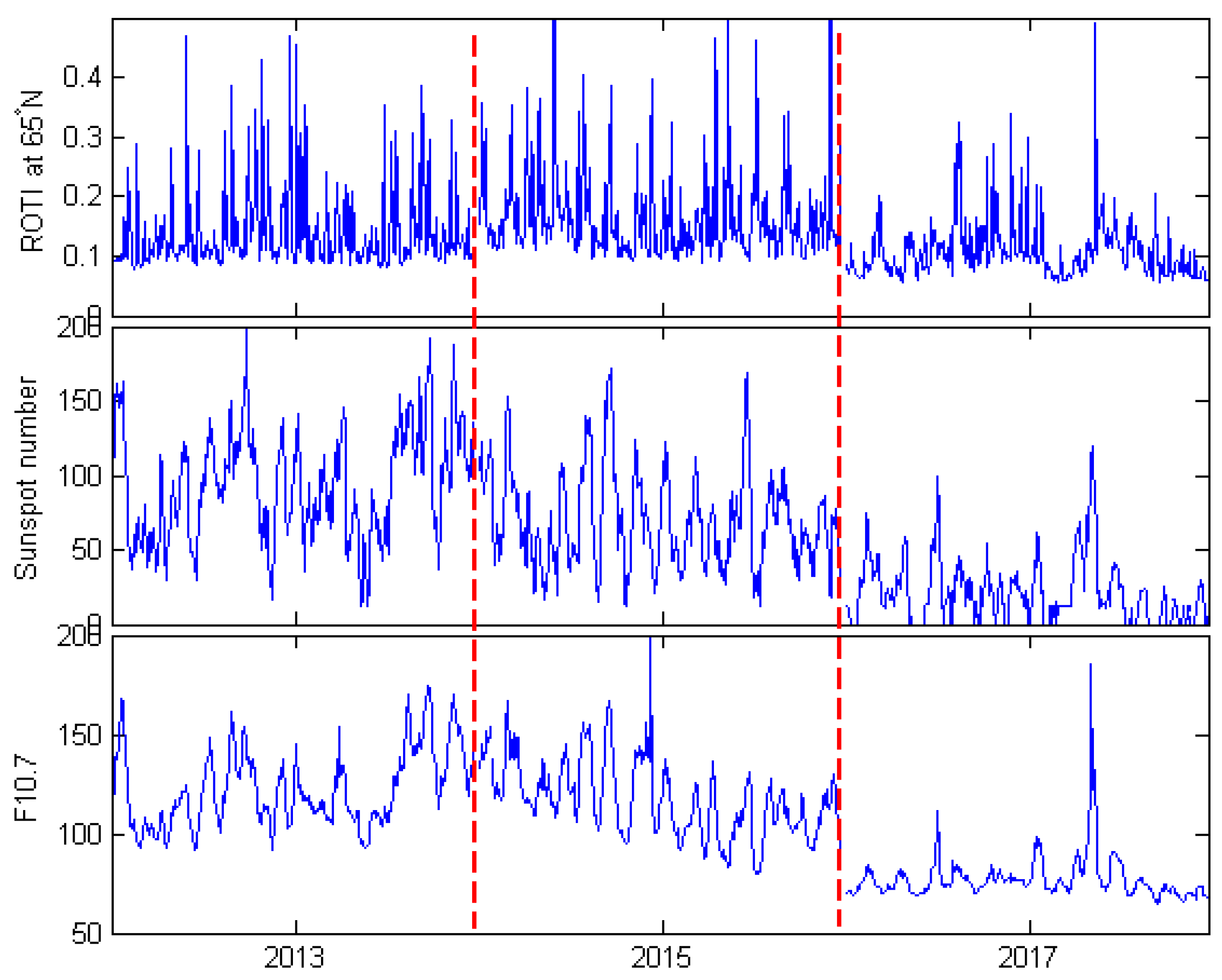
Results for 2013, 2015, and 2017 were selected from the whole 11-year dataset, as the most representatives to analyze the solar activity’s impact on the ROTI performance–selected years cover ascending and descending phases of the solar activity and first part of the solar cycle maximum at the turn of 2013 and 2014. During the above-mentioned periods there also occurred several severe geomagnetic storms. High latitude ROTI—especially in the long scales—reveals sensitivity to the solar conditions. In Figure 3 there is a three-year daily ROTI time-series (for the 65${}^{°}$N of magnetic latitude) compared with the daily average sunspot number and F10.7 index.

Although not every peak value in solar indices has a direct counterpart in the high-latitude ROTI values, Figure 3 clearly shows that during low solar activity (2017) the ROTI values are generally lower.

As we assessed the ROTI performance to describe ionospheric irregularity occurrences for various magnetic local time conditions, we converted geographic positions (GLAT, GLON) of the selected stations to magnetic coordinates (MLat, MLon). We also superimposed magnetic isolines in the station map in Figure 1. Sets of geographic and geomagnetic coordinates are shown in

Table 1. Geographic and geomagnetic positions of the considered European stations (in degrees).

Station ID	GLAT	GLON	MLAT	MLon
TRO1	69.663	18.940	67.115	102.790
VIL0	64.698	16.560	62.069	97.596
MAR6	60.595	17.259	57.623	96.175
VIS0	57.654	18.367	54.343	95.952
BUDP	55.739	12.500	52.326	90.331
REDZ	54.472	17.118	50.768	93.853
BYDG	53.135	17.994	49.209	94.214
BOR1	52.277	17.073	48.223	93.182
GOPE	49.914	14.786	45.424	90.588
TUBO	49.206	16.593	44.579	91.996
LINZ	48.310	14.283	43.466	89.771
GRAZ	47.067	15.493	41.961	90.560
GSR1	46.048	14.544	40.681	89.508
UNPG	43.119	12.356	36.849	87.015
AQUI	42.368	13.350	35.923	87.770
M0SE	41.893	12.493	35.249	86.923
MATE	40.649	16.704	33.898	90.510
LAMP	35.500	12.606	26.469	86.179

for the European sector and

Table 2. Geographic and geomagnetic positions of the considered North-American stations (in degrees).

Station ID	GLAT	GLON	MLat	MLon
RESO	74.691	−94.894	82.570	326.490
BAKE	64.318	−96.002	72.630	330.740
TKTO	62.490	−103.282	70.110	319.920
ENNA	60.767	−101.696	68.610	320.130
CHUR	58.759	−94.089	67.340	331.150
FLIN	54.726	−101.978	62.660	322.600
SASK	52.196	−106.398	59.710	318.140
DUBO	50.259	−95.866	58.790	331.460
P055	47.117	−104.685	54.890	321.700
P054	45.846	−104.441	53.660	322.300
ECSD	43.734	−96.614	52.260	331.880
P042	42.052	−104.911	49.860	322.610
P044	40.172	−103.222	48.160	324.900
P037	38.422	−105.105	46.250	323.090
P123	36.635	−105.911	44.400	322.510
WMOK	34.738	−98.781	43.160	330.760
P027	32.802	−105.804	40.610	323.250
P807	30.495	−98.822	38.940	331.250

for the North-American one.

After collecting a set of RINEX observation files, we calculated ROTI series for each station with the following steps:

• We examined the quality of the RINEX files, data gaps, and a number of cycle slips.
• We calculated ROT values using Equation (3) (taking STEC values for the epoch $t_i$ and $t_{i-2}$, as we used standard 30-s RINEX files), taking the 30-degree cutoff mask for the elevation angle.
• We calculated ROTI values using a 5-min running window with the checking of the observation arc continuity assessment—for each epoch t we included into the calculation ROT values from the previous 5 min, while taking the possibility of observing lags into account as well.
• We calculated 5-min ROTI average values within 2 degree by 2 degree cells above each station.
• We calculated hourly, day-time, and nighttime LT average ROTI values.

Finally, the derived year-long ROTI series of ROTI values for each year and each station were reorganized into keogram-like time series as a function of time and latitude, with subsequent days of the year on the horizontal axis, latitude on the vertical axis, and the corresponding ROTI values from 0 up to 1 on the TECU/min color scale.

In order to evaluate relationships of ionospheric irregularities detected by GNSS ROTI with geomagnetic conditions, we also analyzed the corresponding time series of the AE index—a measure of global electrojet activity based on the measurements from observatories located in the auroral area [31]; and the Ap index denoting the disturbances in the Earth’s magnetic field on a global scale, which can also be treated as the auroral oval spread measure. Indices were turned into hourly and daily averages.

Currently there exist few models of the auroral oval ionosphere and the ROTI product could be their reasonable supplement. Additionally, the International Reference Ionosphere (IRI)—although it does not include ionospheric irregularities in any form—had an auroral oval model implemented [32].

To assess the latitudinal distribution of the enhanced ROTI-described irregularities we included the Zhang and Paxton auroral oval model [33] for comparison. This model—included a few years ago into the most recent version of the IRI model [34]—is based on the observations performed by the Global Ultraviolet Imager (GUVI) settled on the Thermosphere Ionosphere Mesosphere Energetics and Dynamics (TIMED) mission spacecraft. The GUVI-based model is completely independent from the GNSS-based model and products.

3. Results

In terms of GNSS ROTI analysis, the ionospheric irregularity phenomenon can be characterized in several ways. The first one is to analyze long-term time-series of ROTI values; the other one is to analyze the equatorward move of the auroral ionospheric irregularity zone.

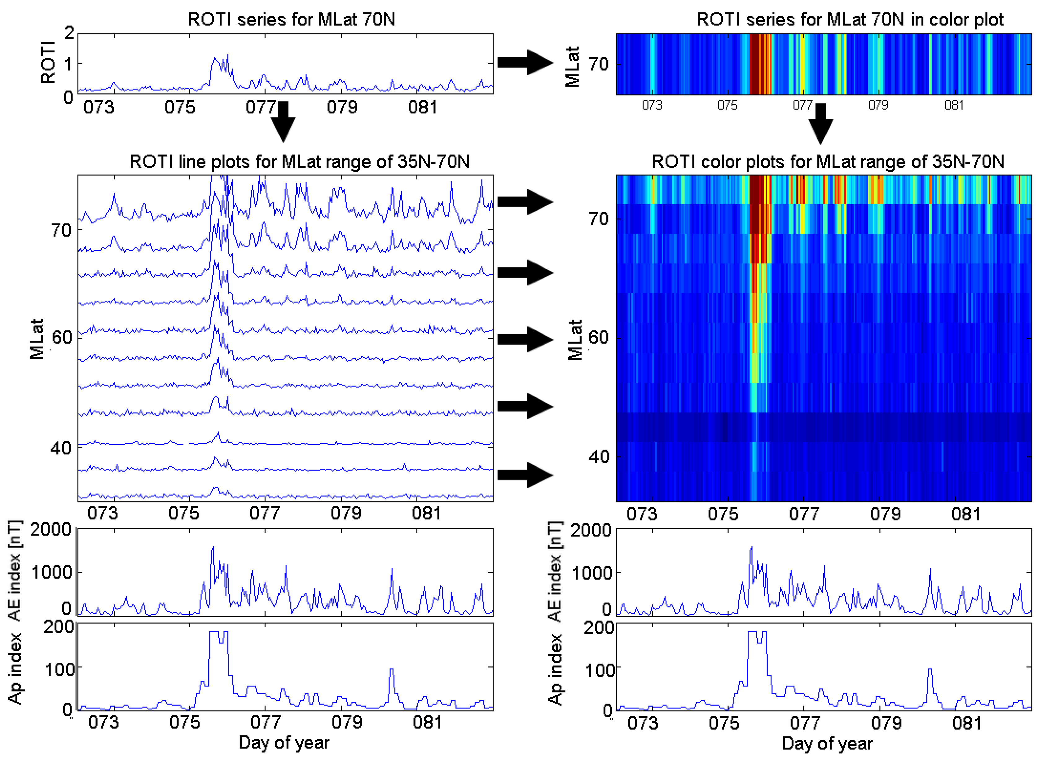
For a more clear presentation, the ROTI series are organized in the form of keogram-like color plots, where ROTI is presented as a function of magnetic latitude and time. Figure 4 shows an example of this projection. Here, time-series of GNSS ROTI values calculated for every station of the latitudinal chain are binned into small cells in magnetic latitude, and U.T.; a color of each cell represents an average intensity of ROTI (blue depicts low intensity, while yellow-to-dark red colors show a high level of ionospheric irregularity intensity).

Previous studies of ROTI behavior at high latitudes [18,19] reported that ionospheric irregularity occurrence signatures, as derived from ground-based GNSS measurements, have a high degree of similarity with the auroral oval location and they can be discussed in terms of general auroral oval dynamics. Considering diurnal ROTI changes at high latitudes and auroral oval dynamics, one can note a clear difference between ROTI intensity during magnetic daytime and nighttime conditions, both in quiet and disturbed ones. To demonstrate the presence of these signatures in long-term series, we split our ROTI results into daytime and nighttime parts in terms of LT.

In the study, we selected the European and North-American latitudinal chains of stations—this allowed us to analyze cross sections of the ionospheric irregularities oval at quite opposite longitudinal sectors. Additionally, the North-American network provides a better covering range towards the north magnetic pole, whereas the European stations have a denser coverage of the magnetic latitudes between 50${}^{°}$N and 70${}^{°}$N.

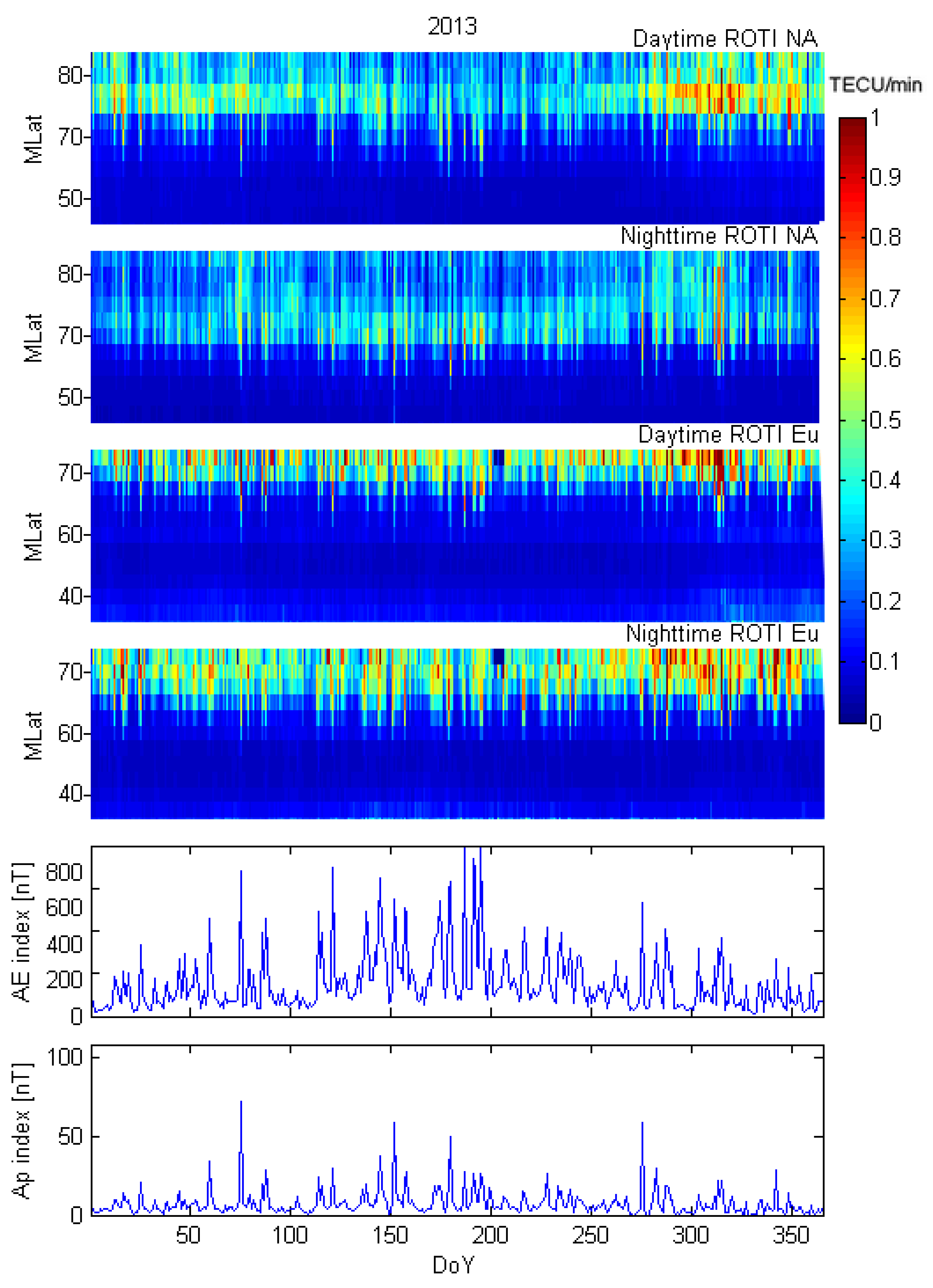
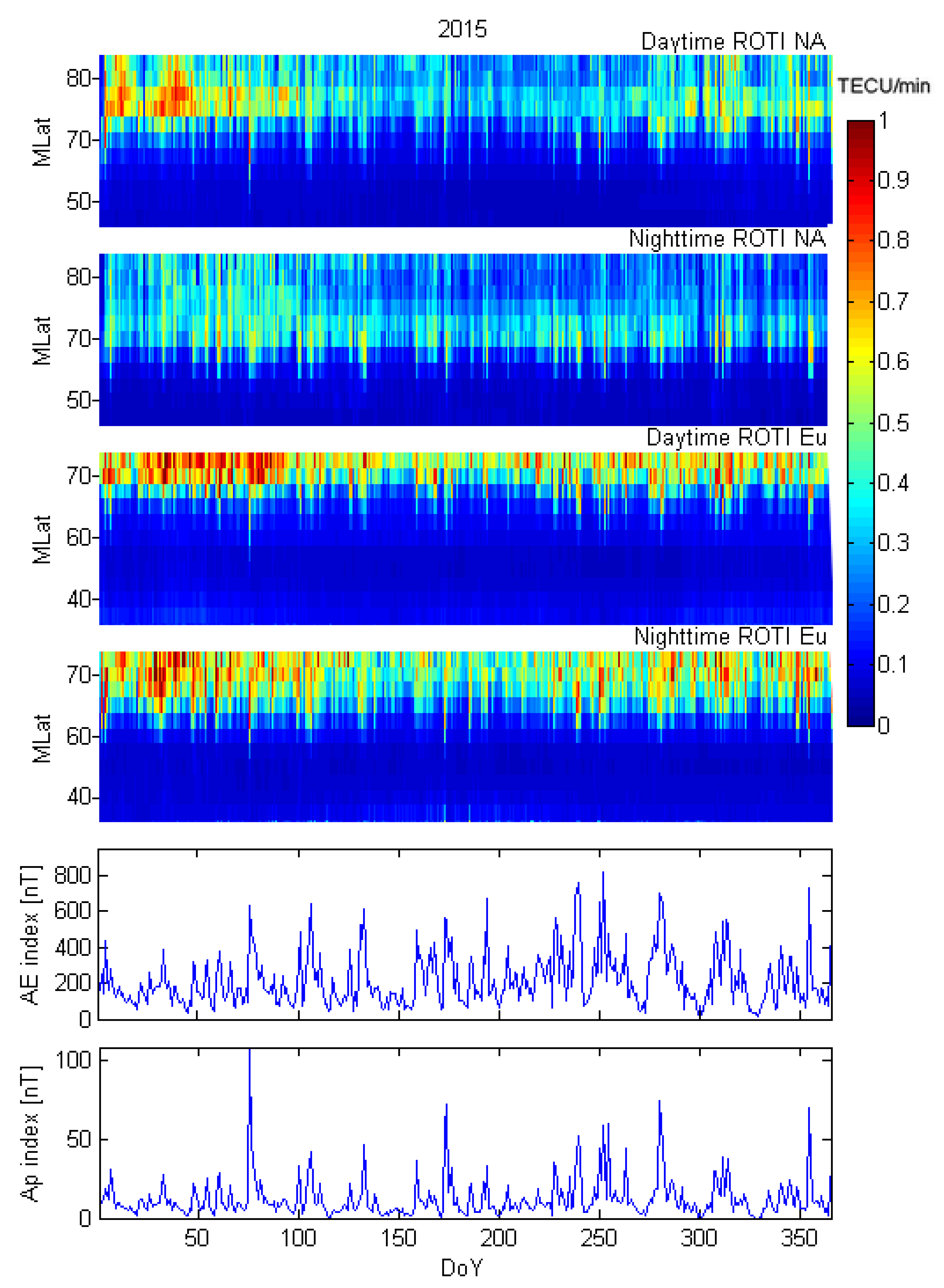
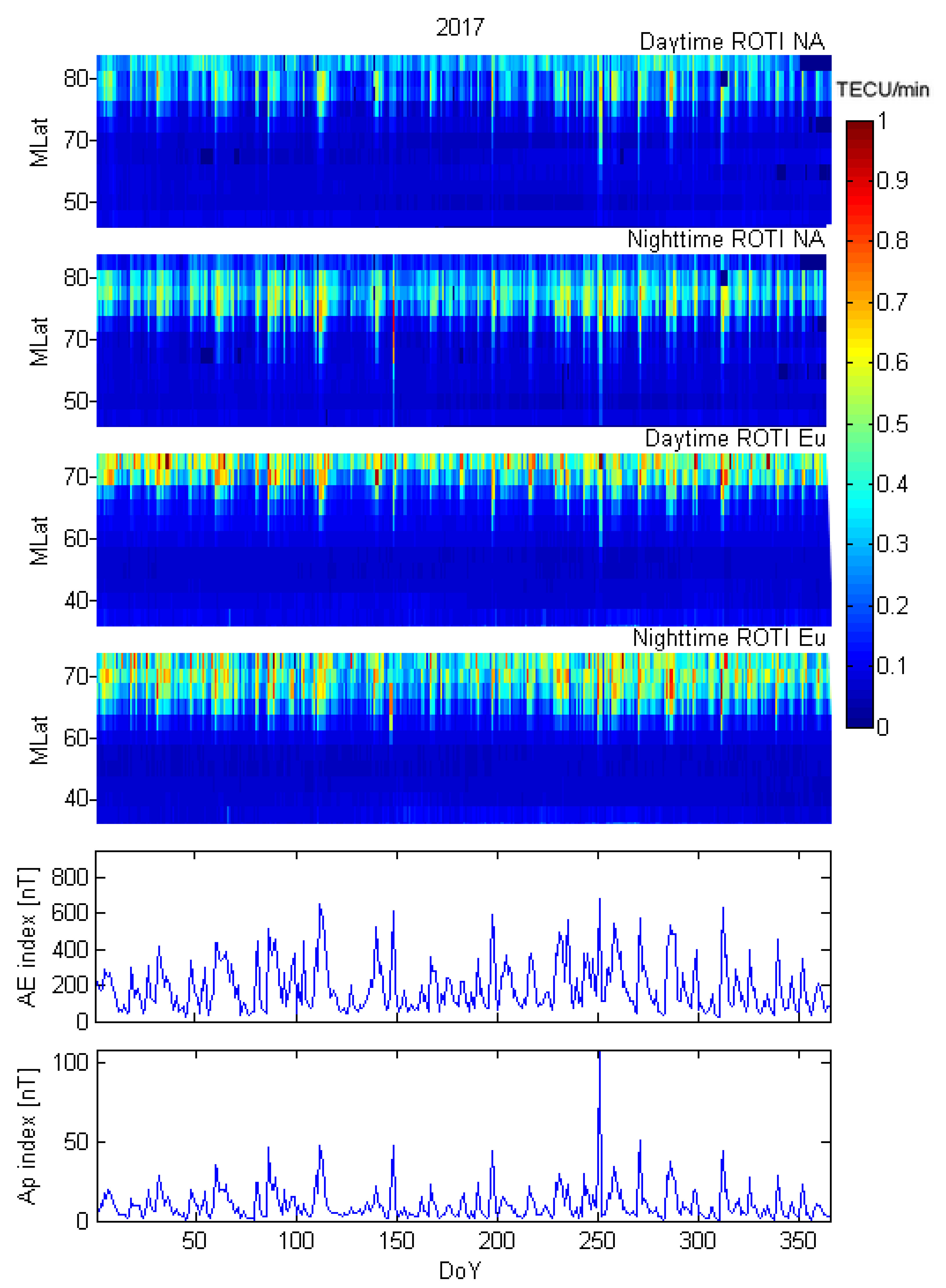
Figure 5, Figure 6 and Figure 7 present the results of the averaged GNSS ROTI variability together with time-series of the AE and Ap indices for years of 2013, 2015, and 2017, respectively. Each of those figures is organized in the following way—the top two panels present ROTI nighttime and daytime time-series for each latitude in the American sector. Two middle panels present the ROTI time-series constructed for the European chain of stations. The last two panels contain time-series of the AE and Ap indices. Such a presentation provides an easy comparison of ROTI behavior in different zones on the background of various geomagnetic activities.

At high latitudes, large magnitudes of GNSS ROTI values are typically associated with the auroral zone of the intense ionospheric irregularities and gradients, forming the so-called “auroral oval” [35]. The auroral oval is expected to form a ring structure surrounding the magnetic pole [36]. Each ROTI time series in Figure 5, Figure 6 and Figure 7 presents a latitudinal slice of the auroral oval, as performed on local day-and night-sides in the European and North-American regions.

The color scale is arranged in the following way to determine the occurrence of the significant ROTI values: The minimal value of ROTI that should be considered as “noticeable” is 0.4 TECU/min. Values below this level are marked with blue and correspond to the state of absence or very weak fluctuation activity. ROTI values above 0.4 TECU/min are marked with light green and move to yellow, then orange, and up to red along with the intensity of the fluctuations. Red corresponds to the ROTI level of 0.9–1.0 TECU/min and above—strong fluctuations that are more typical for intense geomagnetic storms. Such presentation makes it clear to distinguish the range of the significant ROTI occurrence range and the remarkable ROTI value enhancements during events.

All presented ROTI series reveal similar quiet-time behavior, but with some differences associated with the solar activity changes. During high solar activity, ROTI values above 0.4 TECU/min were observed at latitudes between ∼70${}^{°}$N and ∼80${}^{°}$N, with an equatorward expansion down to ∼65${}^{°}$N during night. During the high solar activity period, the ROTI values above 0.5 TECU/min were observed almost every day. During low solar activity (2017), ROTI values were overall smaller and located within a more narrow latitudinal range—between 75${}^{°}$N and 80${}^{°}$N during the day and 70${}^{°}$N and 80${}^{°}$N MLat at night.

In general, an average position of the auroral ionospheric irregularities’ equatorward boundary typically varies near 70–75${}^{°}$N of geomagnetic latitude during local daytime and around 65–70${}^{°}$N during local nighttime conditions.

The color plots of the ROTI series reveal a “spiked structure”—the downward spikes corresponding with the occasional equatorward expansion of the high ROTI values during intense geomagnetic activity events.

Peaking values of both Ap and AE indices have an immediate response in ROTI enhancements at high latitudes and increased ROTI value occurrences at much lower latitudes. We selected several of the highest values of the Ap index in each analyzed year and compared them with AE values, ROTI maxima, and the high ROTI values (

Table 3. High Ap and AE values compared with ROTI behavior (maximum value and equatorward spread).

Date of the Event	Ap (Daily)	Ap max	AE (Daily) [nT]	AE max [nT]	Daily ROTI Peak	Lowest MLat of High ROTI
2013/076	72	111	684	2571	1.0735	55${}^{°}$N
2013/152	58	132	546	1645	0.7331	60${}^{°}$N
2013/275	58	179	528	2087	0.9189	55${}^{°}$N
2015/076	108	179	633	2269	0.8900	50${}^{°}$N
2015/174	72	179	555	2212	0.7207	55${}^{°}$N
2015/280	74	154	697	1839	0.7484	60${}^{°}$N
2015/354	70	111	726	1946	0.9969	55${}^{°}$N
2017/148	47	132	617	1960	0.6777	60${}^{°}$N
2017/197	44	80	590	1748	0.7097	60${}^{°}$N
2017/251	106	236	677	2677	1.1066	50${}^{°}$N

).

Table 3 clearly shows that stronger geomagnetic events (with AE exceeding values of 2000 nT triggering a stronger response in ROTI values and high ROTI spreading towards the equator.

In the European sector, due to the station distribution, the latitudinal slices of ROTI cover mainly the low-to-mid part of the auroral irregularity oval. In the North-American sector with a more favorable configuration of GNSS stations—the ROTI observations reveal a clear poleward boundary of the auroral irregularity oval around 80–85${}^{°}$N during local daytime and down to 75${}^{°}$N during local nighttime conditions, depending on the season and solar cycle phase. The poleward boundary of the auroral oval is also vulnerable to the disruptions caused by intense geomagnetic activity. The poleward boundary moves further poleward during severe geomagnetic storms.

We found that the ROTI daily average values were larger in the second half of the year 2013 and the first half of 2015. There were no significant enhancements in the geomagnetic indices, but these periods are around the 24th solar cycle maximum (at the turn of 2013 and 2014, as shown in Figure 1) and thus the background TEC was also larger.

In order to illustrate the diurnal variability of ROTI-based characteristics of ionospheric irregularities’ occurrence, we calculated ROTI hourly averages; and taking into account the seasonal variation as well, we divided the results into separate seasons (centered for March, June, September, and December). The seasonal averages can be treated as quiet-time ionosphere description, as the considered 24th solar cycle was characterized by moderate/low overall activity, so occasional geomagnetic events were smoothed-out by three-month averaging.

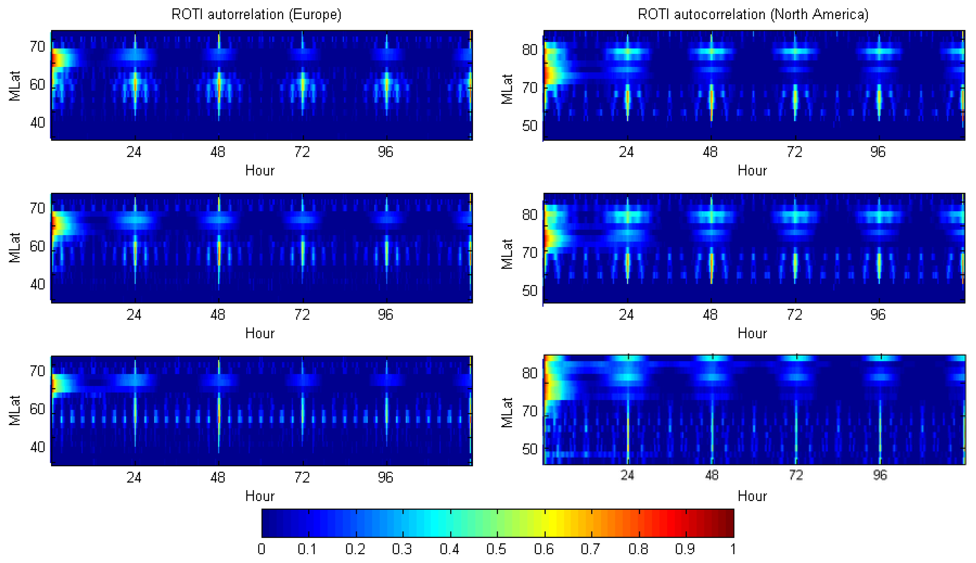
Presented annual sets of daytime/nighttime ROTI observations also demonstrate some characteristics of the seasonal and annual variability of the high-latitude ionospheric irregularities’ occurrence, but the used 12-h averaging potentially whites out all daily variations (besides most general day–night differences). In order to examine the day-to-day changes and repeatability of the ionospheric irregularities patterns, we calculated the autocorrelation of each latitudinal ROTI time-series. For a detailed analysis, we used the basic 5-min data. The derived autocorrelation results for the European and North-American sectors for the years of 2013, 2015, and 2017 subsequently are shown in Figure 8.

The autocorrelation analysis shows in the first place a strong autocorrelation for the lags of 24, 48 h, and the following 24-h multiples. Values for those lags exceed level of 0.6. This makes it possible to conclude that there is a daily repeatable pattern in the ROTI time-series; however, this is only valid for middle geomagnetic latitudes (below 60–70${}^{°}$N), so below the area of strong ionospheric irregularities’ occurrence. At high latitudes, the autocorrelation seems to be blurred and high values occur only for lags below 2 h. The low-to-intense ionospheric irregularities are present almost all the time within the auroral oval zone independently of the geomagnetic and solar activity level (cf., Figure 9). Additionally, some autocorrelations could be spotted for ∼3-h lags; however, their values do not exceed the level of 0.4.

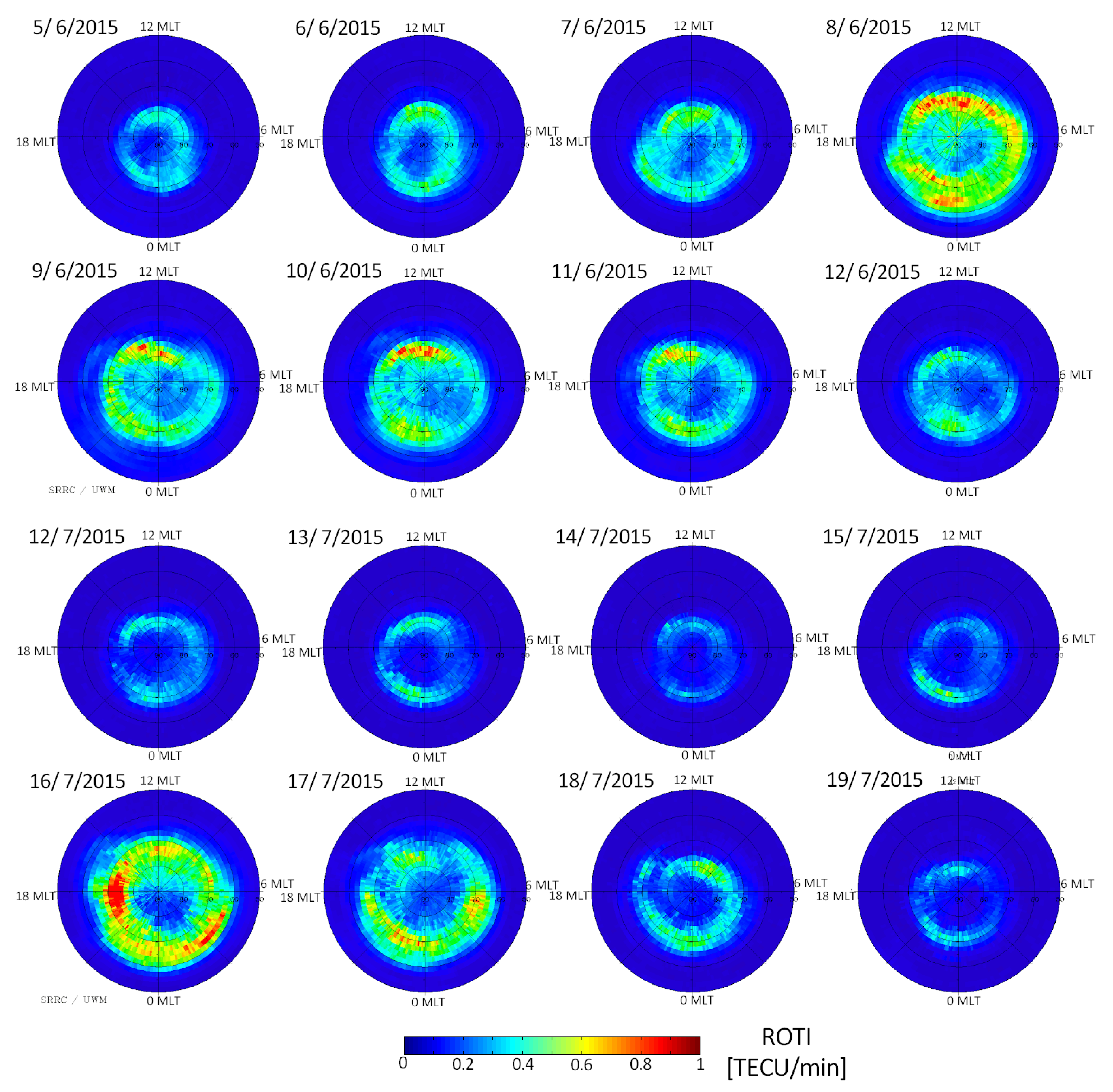
Figure 9 shows several examples of the IGS ROTI maps in a polar view illustrating the auroral oval of the ionospheric irregularities as derived from multi-station GNSS observations. The maps were constructed in the 00–24 magnetic local time (MLT) domain.

The sequence of the diurnal ROTI maps presented an evolution of the ionospheric irregularities oval before, during, and after moderate geomagnetic storms. At the background quiet time, the ionospheric irregularities were found to be more pronounced during a high solar activity period (year of 2015). The intensity, shape, and location of the irregularities oval during disturbed conditions mainly depend on geomagnetic storm’s intensity and duration for both low and high solar activity periods.

Despite different conditions of solar activity level, it can be noted that ionospheric irregularities of moderate intensity are observed permanently within the oval, which explains a low day-to-day autocorrelation (on 24-h lags), as presented in Figure 8. The oval is also stretched more equatorwards at the night side and reaches latitudes of 60${}^{°}$–70${}^{°}$N MLat—similarly to the results presented in Figure 5, Figure 6 and Figure 7. Figure 8 demonstrated that there should be a daily repeatability of ROTI patterns seen (at least for latitudes below 70${}^{°}$N), and we examined the daily variability signatures in more detail (below).

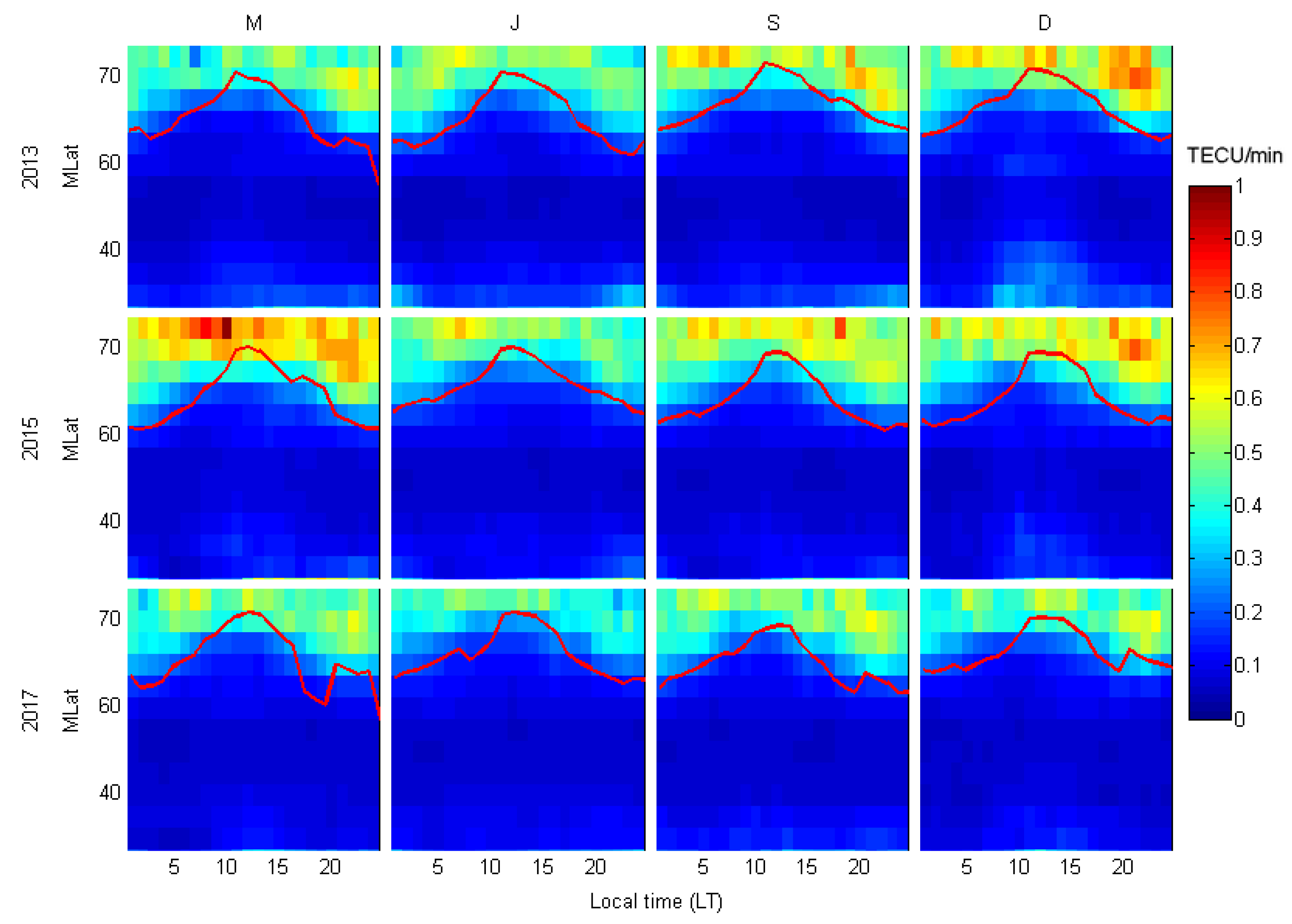
To analyze the average characteristics of diurnal ROTI variability, we calculated the hourly ROTI averages in terms of L.T., taking into account different seasons—the entire dataset was divided into twelve subsets: four seasonal (March, June, September, and December-centered) subsets for every year. The seasonal averages can be treated as quiet-time ionosphere descriptions, as the considered 24th solar cycle was characterized by moderate/low overall activity, so occasional geomagnetic events were smoothed-out by the applied three-month averaging. Figure 10 and Figure 11 present the results for the European and the North-American regions, respectively. For every seasonal subplot, we also superimposed the equatorward boundary of the auroral oval, as derived from the Zhang and Paxton [33] empirical model of the auroral oval that was implemented into the recent version of the International Reference Ionosphere—IRI-2016 [34]. This model is a Kp-dependent global auroral model developed based on global far ultraviolet auroral data collected by Thermosphere Ionosphere Mesosphere Energetics and Dynamics (TIMED)/Global Ultraviolet Imager (GUVI).

The seasonal averages of hourly ROTI values presented as a function of MLT and MLat in Figure 10 and Figure 11 demonstrate a similar daily trend as single-day observations (Figure 9)—the equatorward boundary of the ionospheric irregularities region expands equatorwards during magnetic night and demonstrates a more poleward location during local daytime. That is a typical behavior of the auroral oval corresponding to the observations and current empirical models of the auroral oval. Additionally, the maximum of ROTI obviously shifts equatorward during local nighttime, as was also shown for ROTI observations in [37], and well agreed with the concept of the auroral oval (e.g., [35,38,39]). A daytime localized ROTI increase close to the magnetic noon can be associated with particle precipitation into the polar cusp region. In Figure 11 one can also note a pronounced drop in the irregularities intensity at higher latitudes (around 80${}^{°}$N) during nighttime—this also corresponds to the quiet-time auroral oval poleward border in Figure 9—irregularities surround the north magnetic pole in a ring-like structure, decreasing significantly in the closest vicinity of the pole [36]. Thus, for the North-American region, the ROTI-based analysis can detect both the poleward and equatorward boundaries of the irregularities oval.

The border is sharper in the local winter half of the year (March and December-centered seasons). Additionally, the average ROTI values were found to be higher during winter seasons. This can be explained by the sunlight conditions during polar day/night which impact quiet-time, large-scale plasma gradient formation at high latitudes.

The winter-summer differences become less evident in 2017 (c.f. June and December results in Figure 8 and Figure 9, when the background ionospheric plasma density level and the whole activity were very low due to the deep solar cycle minimum). During the whole 2017, the ionospheric irregularities oval was narrower—about five degrees closer to the north magnetic pole—than that of the years with a higher solar activity level.

Additionally, we note that the latitudinal spread of the irregularities oval corresponds well to the equatorward border of the auroral oval derived from the Zhang and Paxton model (red lines in Figure 8 and Figure 9.

Thus, our results confirm repeatable signatures of ROTI occurrence at high latitudes as observational evidence for presence of low-to-moderate intensity ionospheric irregularities within the auroral oval zone at all levels of solar activity and quiet-time conditions. The most dramatic intensification of ROTI at high latitudes is usually a result of geomagnetic activity increases.

As it was shown in Figure 5, Figure 6 and Figure 7, jumping values of AE and Ap indices have a direct response in ROTI results, both in the magnitude and in the expansion of latitudinal range of high ROTI values. To examine the latitudinal dependence of ROTI on geomagnetic conditions in more detail, we calculated linear correlation coefficients between the AE index and each latitudinal ROTI time-series. 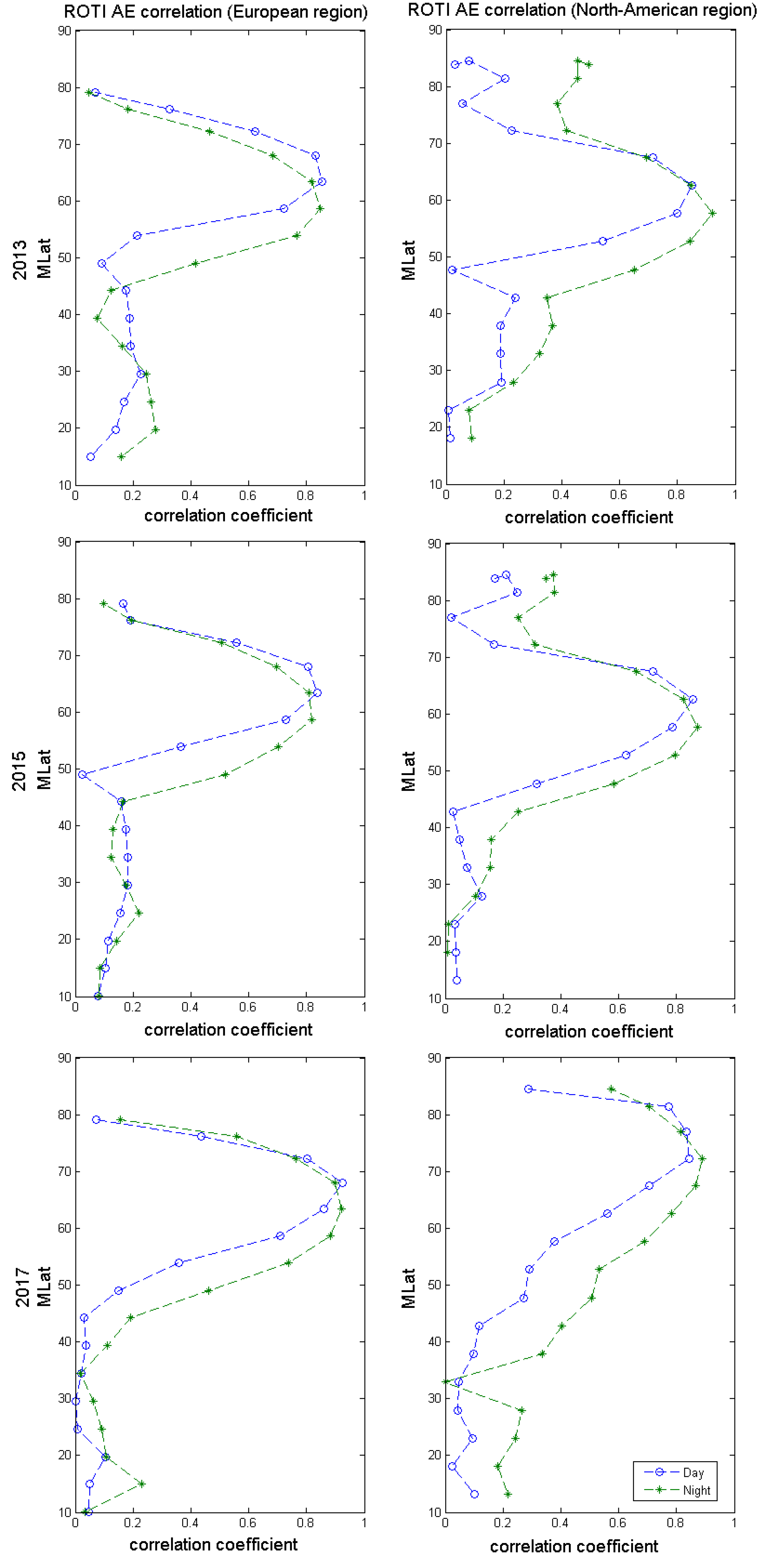Figure 12 presents results of correlation analysis between the AE index and ROTI values for the European and North-American sectors for different years.

The results in Figure 12 demonstrate that the linear correlation coefficient reaches the largest values at high latitudes (above ∼55–60${}^{°}$N). This correlation is considered as a strong one. The largest values (R∼0.8) are registered within a narrow latitudinal range of ∼60${}^{°}$N–70${}^{°}$N, but large values of correlation (R > 0.6) are found at lower latitudes down to ∼50–55${}^{°}$N, depending on the conditions. It is interesting to note that poleward of 70${}^{°}$N MLat, the correlation value rapidly drops below 0.4 in both longitudinal sectors. Thus, the most pronounced correlation between the AE index and ROTI was found within a relatively narrow latitudinal zone of 55–70${}^{°}$N MLat—that means that ROTI displays a selective latitudinal sensitivity and with a rapid AE increase; the ROTI magnitude increase should be expected mostly within this zone, associated with an auroral oval expansion. This confirms that occurrences of intense ionospheric irregularities within the auroral oval are driven mostly by geomagnetic factors.

A general view on the ROTI series in Figure 5, Figure 6 and Figure 7 reveals a noticeable equatorward move of the irregularities zone that corresponds to the night-side spread of the auroral oval. It has straightforward equivalence in the ROTI/AE correlation. The high correlation bulge in all plots is more extended for the nighttime data—night ROTI is more sensitive to geomagnetic activity independently of the sector and solar cycle phase. Additionally, during high solar activity, ROTI sensitivity to AE index spreads further equatorward.

Occurrence of mid-latitude plasma density structures in the ionosphere and the auroral oval expansion towards middle latitudes are mostly driven by geomagnetic activity, whereas at high geomagnetic latitudes, ionospheric irregularities occur most of the time within the auroral oval zone—high geomagnetic activity enhances their strength and the size of this zone.

4. Discussion and Conclusions

In this study, we analyzed three representative year-long periods based on time series of the GNSS-based ROTI values in two sectors—European and North-American—in order to assess the climatological characteristics of mid and high-latitude ionospheric irregularities. We have assessed the ROTI-described ionospheric irregularities in of the daily variation and daily repeatability, seasonal and solar cycle variations, and correlations with indices describing magnitudes of geomagnetic disturbances to find the climatological signatures of the ROTI-derived TEC fluctuations.

The long-term analysis of ROTI shows that the GNSS technique could be successfully used to describe the morphology and evolution of the ionospheric irregularities. ROTI is quite sensitive to rapid changes in the geomagnetic conditions. Thus, ROTI can be used to describe quiet-time ionospheric irregularity occurrences and to characterize GNSS signal fluctuation level enhancement, and its spatial expansion during serious geomagnetic events of different intensity.

Since phase fluctuations detected by ROTI are related to radio signal scintillations, the ROTI data product can be a very useful tool to describe ionospheric plasma density irregularity occurrences on a global scale. This technique does not require any additional equipment, aside from currently present and widely-available GNSS permanent networks.

Many of the GNSS scintillation studies are devoted to the signal amplitude scintillations. There is observational evidence that signal amplitude scintillations are rather rare in the polar zone—signal phase scintillations are more typical for this region. Thus, for mid-to-high latitudes, it is of crucial importance to perform a continuous monitoring of phase fluctuation activity based on GNSS observations. We also emphasize that climatological ROTI characteristics obtained in this study are in very good agreement with the high rate phase scintillation ($\sigma \varphi$, sigma phi) climatology at the high and subpolar latitudes [40]. Similar correspondence can be found in amplitude scintillation studies—despite the fact that intensity scintillations are more typical for the equatorial zone, there are also signatures of intensity scintillation occurrence within the auroral oval zone [41].

The average quiet-time ROTI climatological characteristics also agreed well with the empirical models describing the auroral oval position. In particular, the IRI-2016 model provides now the equatorward boundary of the auroral oval derived from the Zhang and Paxton empirical model [33]. The diurnal variation of the polar region irregularities specified by ROTI demonstrated that these irregularities mainly occur within auroral oval boundaries, as determined by this empirical model. Both the noticeable ROTI and auroral oval boundary variations demonstrate similar behavior with with the seasonal and solar cycle variations. This agreement is equally strong at both longitudinal sectors (European and North-American).

Currently, the IGS provides ROTI maps for the Northern hemisphere—a product, specified the daily ROTI pattern at high latitudes [19]. In Figure 9, we demonstrate several examples of the diurnal behavior of the ionospheric irregularity oval in different conditions. In this work, we assessed the ROTI behavior in long-term, climatological scales and found a clear correlation of our results with the single (quiet or disturbed) day IGS ROTI maps.

For our long-term analysis, we considered spatio-temporal variability of ROTI along two specific longitudes, which represent cuts of the auroral irregularity oval at two different sectors. This geographical separation allowed us to perform the analysis for two sectors with dense and broad networks of GNSS users in the Northern hemisphere. We recognized the important characteristics of the ionospheric irregularity pattern in quiet and disturbed conditions. For all levels of solar activity, an obvious prevailing of ionospheric irregularity occurrences at local night-side was registered. The equatorward border of the irregularities zone is typically located at lower latitudes during local nighttime—around five degrees lower than those of daytime. This also agreed well with the phase scintillation climatology [40]—despite a maximum probability of phase scintillation occurrence appearing around noon, the overall enhanced probability is shifted further equatorward during nighttime.

A number of authors have utilized ROTI during specific case-studies of intense geomagnetic storms [21,42,43]. Climatological characteristics specified by average ROTI values reveal also a clear sensitivity to the geomagnetic activity disturbances (as proven on example of AE and ap indices). Geomagnetic events trigger a direct response in irregularities patterns described by ROTI—the maximum value rises and the zone of enhanced ROTI value spreads equatorward, reaching mid-latitudes. During intense geomagnetic activity events, the ROTI magnitude reaches larger values of 1 TECU/min and above, whereas the irregularities zone expands equatorward down to even 50${}^{°}$N MLat depending on the storm magnitude. The pronounced asymmetrical day-side/night-side oval stretch is driven by the geomagnetic conditions (e.g., IMF By) and the specific time of the storm commencement.

Results of our analysis confirm a very good performance of the ROTI-based approach for characterization of the ionospheric plasma irregularities climatology in the mid and high-latitude regions. ROTI values describe very well the temporal and spatial evolution of the ionospheric irregularities within the auroral region during the local day–night cycle at non-disturbed conditions. These results also confirmed a rather high sensitivity of the ROTI index in detecting and specifying features of plasma irregularity occurrences against seasonal changes and solar ionisation level during the period we examined.

One of the most solid directions now is the existing opportunity of a near-real-time nowcasting of the ionospheric fluctuations with ROTI maps obtained with rapid, multi-site RINEX data. We can consider the ROTI technique as a pure data-driven model and a good candidate for a near-real-time nowcaster of the ionospheric irregularities’ occurrence, limited only by the data availability (data streaming) and hardware capacity. Furthermore, the existing historical GNSS observations and ROTI products have great potential to serve as valuable datasets for assessments and evaluations of currently used models for auroral oval location and boundaries. Since ROTI is derived directly from the radio beacon observations, we also aim to perform a comparison with other types of radio signal measurement, e.g., radio astronomical observations. In particular, the Low Frequency Array (LOFAR) telescope performs observations in low radio frequencies that are very vulnerable to ionospheric disturbances. Simultaneous observations of astronomical radio sources, such as supernova remnant Casiopeia A, radio galaxy Gygnus A, and bright pulsars, together with ground-based GNSS ROTI observations could bring fascinating insights to the morphologies of ionospheric disturbances’ impacts on different radio frequencies.