Decoding Complex Erosion Responses for the Mitigation of Coastal Rockfall Hazards Using Repeat Terrestrial LiDAR

Abstract

A key factor limiting our understanding of rock slope behavior and associated geohazards is the interaction between internal and external system controls on the nature, rates, and timing of rockfall activity. We use high-resolution, monthly terrestrial light detection and ranging (LiDAR) surveys over a 2 year monitoring period to quantify rockfall patterns across a 0.6 km-long (15.3 × 10³ m²) section of a limestone rock cliff on the northeast coast of England, where uncertainty in rates of change threaten the effective planning and operational management of a key coastal cliff top road. Internal system controls, such as cliff material characteristics and foreshore geometry, dictate rockfall characteristics and background patterns of activity and demonstrate that layer-specific analyses of rockfall inventories and sequencing patterns are essential to better understand the timing and nature of rockfall risks. The influence of external environmental controls, notably storm activity, is also evaluated, and increased storminess corresponds to detectable rises in both total and mean rockfall volume and the volumetric contribution of large (>10 m³) rockfalls at the cliff top during these periods. Transient convergence of the cumulative magnitude–frequency power law scaling exponent (ɑ) during high magnitude events signals a uniform erosion response across the wider cliff system that applies to all lithologies. The tracking of rockfall distribution metrics from repeat terrestrial LiDAR in this way demonstrably improves the ability to identify, monitor, and forecast short-term variations in rockfall hazards, and, as such, provides a powerful new approach for mitigating the threats and impacts of coastal erosion.

1. Introduction

Rockfall, or the removal of individual and superficial rocks from a cliff face [1,2], is a significant geohazard, particularly on coastal cliffs where the exposure of people and assets is often high [3,4]. Rock coasts account for much of the world’s coastline [5], yet our understanding of their evolution remains limited by progressive time-dependent failure processes [6], geological and geometric settings [7,8,9], increasing environmental extremes [10,11], and the appropriateness of the available data [12]. A review by Naylor et al. [13] highlighted the need for continued deployment of field techniques to better quantify the relative contributions of different processes and forces in driving rock coast evolution. Similarly, Kennedy et al. [14] highlighted the existence of a key spatiotemporal gap in rocky coast research related to geomorphological processes over seasonal to annual timescales and across distances of 10²–10³ m, scales particularly relevant to coastal management and hazard mitigation.

The last two decades have seen the increasing application of high-resolution topographic data for coastal research [10,15,16,17,18,19,20]. Topographic change detection methods, often employing repeat light detection and ranging (LiDAR) data, have provided valuable insights into rockfall frequency and magnitude [12,16,21,22,23,24,25,26] and enabled links between cliff failure mechanisms and erosional processes to be explored [4,27]. However, the correlation of failure occurrence with specific triggers is complicated by time-dependent deterioration [6], stress release and propagation [28,29], and lagged, cumulative, or threshold effects [30], which have limited the establishment of robust, predictive driver-response relationships. Primarily due to limitations in resources, terrestrial LiDAR methods have typically been used to survey rock coasts across length scales of ~10¹–10³ m. For example, recent work by Esposito et al. [31] utilized repeat terrestrial LiDAR and change detection methods to quantify recession of a ~1 km-long volcaniclastic sea cliff in southern Italy over a 3 year survey interval. They found that most rockfall event volumes that were detected at this spatiotemporal resolution were between 0.01 and 1 m³ and that a seawall structure was effective at reducing erosion driven directly by marine action at the cliff toe, demonstrating the utility of LiDAR-based studies for evaluating the efficacy of coastal defense engineering. To overcome the spatial constrictions of ground-based LiDAR, Benjamin et al. [32] utilized annual helicopter-based LiDAR and change detection methods to detect rockfall activity across a regional (20.5 km) spatial scale for coastal cliffs along the North Yorkshire coast, England, and found that variations in rockfall shape with volume could provide insights into the underlying mechanisms of detachment with scale, and that the role of cliff retreat via large and infrequent (or ‘episodic’) failure can be significant for rocky coastlines, in contrast with the commonly held view that these landscapes are relatively stable.

Key questions still remain as to the geomorphic role of storms on rock cliffs and their efficacy relative to more systematic environmental variations, such as seasonality. This paper analyzes spatiotemporal erosion dynamics for a ~0.6 km-long section of limestone coast in northeast England. We quantified the location, magnitude, and frequency of rockfalls and cliff instabilities over a ~2 year period using repeat terrestrial LiDAR surveys combined with digital elevation model (DEM) differencing. These data were used to consider a range of explanatory variables including lithology, the local protective capacity of shore morphology, and subaerial and marine environmental drivers for dictating short- to medium-term erosion response, and the wider implications of our findings for coastal management and geohazard assessment.

2. Materials and Methods

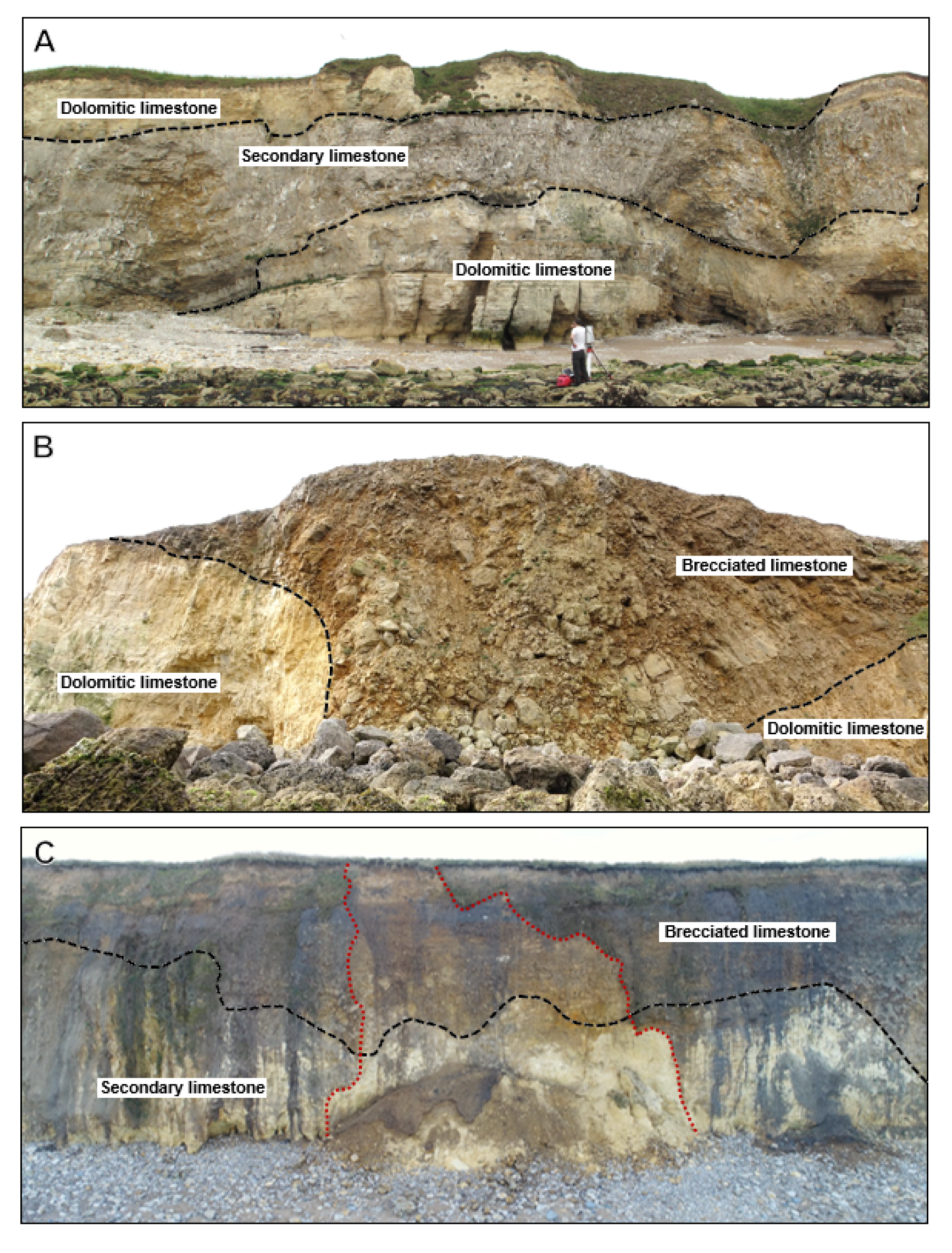
Briefly, our methods comprised: (i) Repeat terrestrial laser scanning and subsequent differencing of these data to detect rockfalls at an approximately monthly timestep; (ii) extraction of detailed rockfall statistics in a Geographic Information Systems (GIS) environment, including rockfall location and timing (i.e., survey interval), lithology, depth, surface area, volume, maximum planar length, spatial density, and intersection with other rockfall events that occurred in the monitoring period; and (iii) a subsequent analysis of these data in the context of the local coastal geomorphology and environmental conditions, and the geohazard potential of the site. Additionally, aerial imagery acquired from an unpiloted aircraft system (UAS) and processed using digital photogrammetry methods were also used to provide additional topographic context for the site (i.e., Figure 1B).

2.1. Study Site

Marsden Bay extends for ~1.5 km along the coastline of northeast England. Its orientation exposes it to fetch distances that exceed 1900 km. Tides range to 5.6 m and the mean and maximum recorded wave height during our monitoring period at the Newbiggin wave buoy, 25 km north of the study site, were 0.9 and 9.8 m, respectively. We focused on a 0.6 km sub-section of the wider bay that includes alternating embayment and headland relief, sub-vertical coastal cliffs with sporadic deep-cut caves, discontinuous sections of uneven shore platform and boulder fields, and pockets of dry pebble and sand beach (Figure 1). The uncertainty surrounding the true rates and responses of the coastal cliffs at three key pinch points has raised concerns over the safe operation of a cliff top coastal road, the A183 that links South Shields to Sunderland [25]. The cliff face is ~25 m in height and is composed of a complex assemblage of dolomitic limestone and dedolomitized limestone. The latter has transformed from limestone to dolomite, and back to limestone via dedolomitization, or re-calcification; we term this lithology ‘secondary limestone.’ Additionally present are concretionary brecciated limestones, formed ca. 252–272 Ma (Figure 2). Dissolution weathering and karstic collapse are evident, resulting in a variety of structural forms ranging from intact to brecciated material, and generally of weak to extremely weak geotechnical competence, which is noted in local borehole inspection reports that could not recover sufficient intact material for strength testing. Dip angles are 41°, 29°, and 47° for the dolomitic, secondary, and brecciated limestones, respectively. Bedding thickness varies between 0.3 and 3 m and is largely horizontal along the cliff face. Joints and fractures tend to be vertical in the dolomitic and secondary limestones but are chaotic in the brecciated limestone. Texturally, the dolomitic limestone is quite open with numerous cavities, rendering it theoretically less competent and prone to weathering than the denser secondary limestone, which, due to its recrystallized nature, possess fewer cavities. Many, but not all, of the brecciated areas are held together with a crystalline cement matrix that adds some cohesion despite the presence of numerous cavities. Further information on the geological context of the site is provided by Smith et al. [33] and Cooper et al. [34]. Contemporary rates of cliff top recession are within manual cliff line survey error, which, in places, can approach or exceed 3 m [35,36]. The predicted future retreat rate of the wider stretch of coastline is 0.1–0.2 m a⁻¹ [34].

2.2. Topographic Data Capture and Rockfall Detection

To capture 3D cliff topography, we used a Riegl LMS-Z620 time-of-flight terrestrial laser scanner (www.riegl.com), set to acquire ~11,000 points per second at a 3D point spacing of 0.05 m at 100 m distance, producing a mean 3D point spacing of 0.03 m. We undertook a total of 24 surveys at an approximately monthly return interval (mean 33.5 days) between February 2015 and March 2017. Each survey comprised three overlapping scans (Figure 1), which were georegistered using: 1) Manual point picking, which achieved cloud-to-cloud alignment to <0.10 m, followed by 2) iterative closest point matching in RiSCAN Pro software (version 1.5.9; www.riegl.com), which works well where the majority of the cliff face undergoes no change between surveys, which is typically the case for coastal cliffs. Final cloud-to-cloud alignment errors were ±0.02 m in xyz. Merged scans for each survey date were then aligned to the earliest terrestrial laser scanner (TLS) survey by repeating steps (1) and (2) above. Compound survey-to-survey alignment errors were ±0.03 m. As the TLS data were not geo-located at the point of acquisition, a differential Global Positioning System (dGPS) and total station survey of twelve distinctive features across the cliff face were used to perform a vertical shift so that cliff elevations were correct relative to a national datum (i.e., meters above Ordnance Datum Newlyn). The same vertical shift was applied to all scans so that the true elevation of rockfall scars could be extracted for subsequent analysis without the computationally expensive use of true easting and northing values in the point cloud data. We used a combination of automatic outlier removal and manual point cloud editing to remove isolated and unwanted points, which comprised seabirds in flight, solar glare, and other artifacts. Due to changes in beach height and slight differences in TLS position in successive surveys, TLS data were clipped at the cliff base to the lowest common vertical extent, which excluded approximately the lowermost 0.7 m of the cliff from our analysis.

We used QT Modeler software (v. 8.0.7.1; www.appliedimagery.com) to convert 3D point cloud data to 2.5D raster digital elevation models (DEMs) at 0.10 m resolution, where the elevation of a grid cell represents the mean of the points contained within it and is thus less susceptible to artificial elevation spikes and noise than if the maximum or minimum point elevation is used. DEMs were imported into ArcGIS software (v. 10.5.1; www.arcgis.com), DEMs were rotated, and successive point clouds (i.e., month 1–month 2, month 2–month 3, etc.) were differenced normally to the cliff face plane to derive the surface change at a detection threshold of 0.10 m, which is deliberately conservative to account for compound scan-to-scan registration errors and geo-location error, and should minimize the likelihood of the smallest rockfall size fractions included being affected by measurement error. This threshold excluded much of the change signal attributable to vegetation growth and dieback, and the growth and disintegration of seabird nests between surveys, which were further manually masked following visual inspection of the point cloud. Changes within areas comprising extreme breaks of slope were removed due to their association with minor data alignment errors and occlusion. These false positives typically took the form of geometrically implausible (i.e., long, thin) instances of change that possessed a volume of ≤0.10 m³.

The mean depth (m) of an erosion scar was multiplied by its 3D surface area (m²; as viewed in the xy plane) to calculate eroded volume (m³). The minimum detectable eroded volume was 1.0 × 10⁻³ m³, a volume that equates to a regular 0.1 m cube. The temporal resolution of field surveys precludes the identification of event superimposition at temporal scales smaller than the revisit interval (e.g., [26]), i.e., where multiple rockfalls occur in the same location within a given survey interval and superimpose to produce a single scar, we are not able to discern the dimensions or timings of the individual rockfalls that it might represent. However, we were able to explore progressive erosion at monthly timescales (Figure 3). We additionally used the FACETS plugin in CloudCompare software (v. 2.10.2; www.danielgm.net) to directly extract geological structure information from the February 2015 3D point cloud. The plugin extracts planar facets; the 2D size, shape, and spatial attitude (e.g., dip) of these facets can be linked to stratification, and the spacing of faults and joints (e.g., [37]). We refer the reader to Dewez et al. [38] for an overview of the plugin.

We additionally acquired an aerial photoset (no. photos = 570) of the wider cliff and foreshore environment on 27 February 2017 using a Phantom 4 Professional UAS (www.dji.com) equipped with an onboard 20-megapixel RGB camera. The purpose of generating a UAS-derived 3D model was for topographic visualization (e.g., Figure 1B) and for the extraction of cliff and shore topographic profiles, which were later used in combination with rockfall location data to explore links between erosion activity and cliff form (Section 3.3). Drone imagery was captured from a combination of oblique (n = 367) and nadir (n = 203) perspectives and was processed using a standard structure-from-motion (SfM) photogrammetry workflow in Agisoft PhotoScan software (version 1.2.6; www.agisoft.com) to create sparse and dense 3D point clouds [39]. Due to tidal conditions at the site and the time required to safely set out and survey a suitably dense ground control point (GCP) network, fly the drone, and retrieve GCPs, it was not logistically possible to use dedicated GCPs for model georeferencing and independent quality assessment. Instead, we employed direct georeferencing (after [40]) using UAS image geotags to generate a DEM from which cliff and foreshore topography were extracted for topographic analysis. With these applications in mind, internal consistency in model geometry was more important than absolute, real-world geolocation. We collected both nadir and oblique imagery, as has elsewhere been shown to mitigate against the introduction of systematic model deformation [41,42]. We anticipate these data to be accurate to ±0.04 m, in line with the findings of Carbonneau and Dietrich [40] who found residual DEM errors equal to 0.1% of flying height (here, ~40 m) when direct georeferencing was used.

2.3. Environmental Data

We retrieved the mean tidal water surface height from the North Shields local tidal reference station, 6 km to the northwest of the study site (via the British Oceanographic Data Centre: www.bodc.ac.uk), and used these data to calculate the duration of tidal cliff toe inundation (Figure 1D) and identify the boundary between ‘wet’ and ‘dry’ zones, and also obtained offshore wave spectra data, specifically the mean and maximum wave height, from the Newbiggin wave buoy (via the Channel Coastal Observatory: www.channelcoast.org). We did not employ wave transformation modeling, which can account for processes such as wave run-up, refraction, and shoaling, and, as such, we do not undertake any quantitative correlation analysis between erosion statistics and wave metrics. However, offshore wave data are useful for indicating relative differences in far-field wave environments over time. We used the tidal water surface data to infer the location of ‘wet’ and ‘dry’ zones on the cliff profile; because we did not account for wave runup, this boundary is, therefore, a conservative one (i.e., in reality, it more than likely occurs higher up the cliff face). In the absence of an on-site or nearby automatic weather station, we retrieved reanalysis meteorological data from the National Oceanic and Atmospheric Administration’s Climate Prediction Center (CPC; www.esrl.noaa.gov), derived from a combination of satellite and weather station data. In line with previous coastal erosion studies that have explored links between rockfall activity and environmental factors (e.g., [10,12]), we chose not to consider air temperature in our analysis. For high-latitude [43] or high-altitude rock slopes [44], persistently low air temperatures are conducive to the growth and influence of ground ice in driving or conditioning erosion activity; however, diurnal or seasonal variations in air temperature are unlikely to be key environmental data for driving erosion at our temperate coastal site, where local air temperatures very rarely drop below freezing.

3. Results

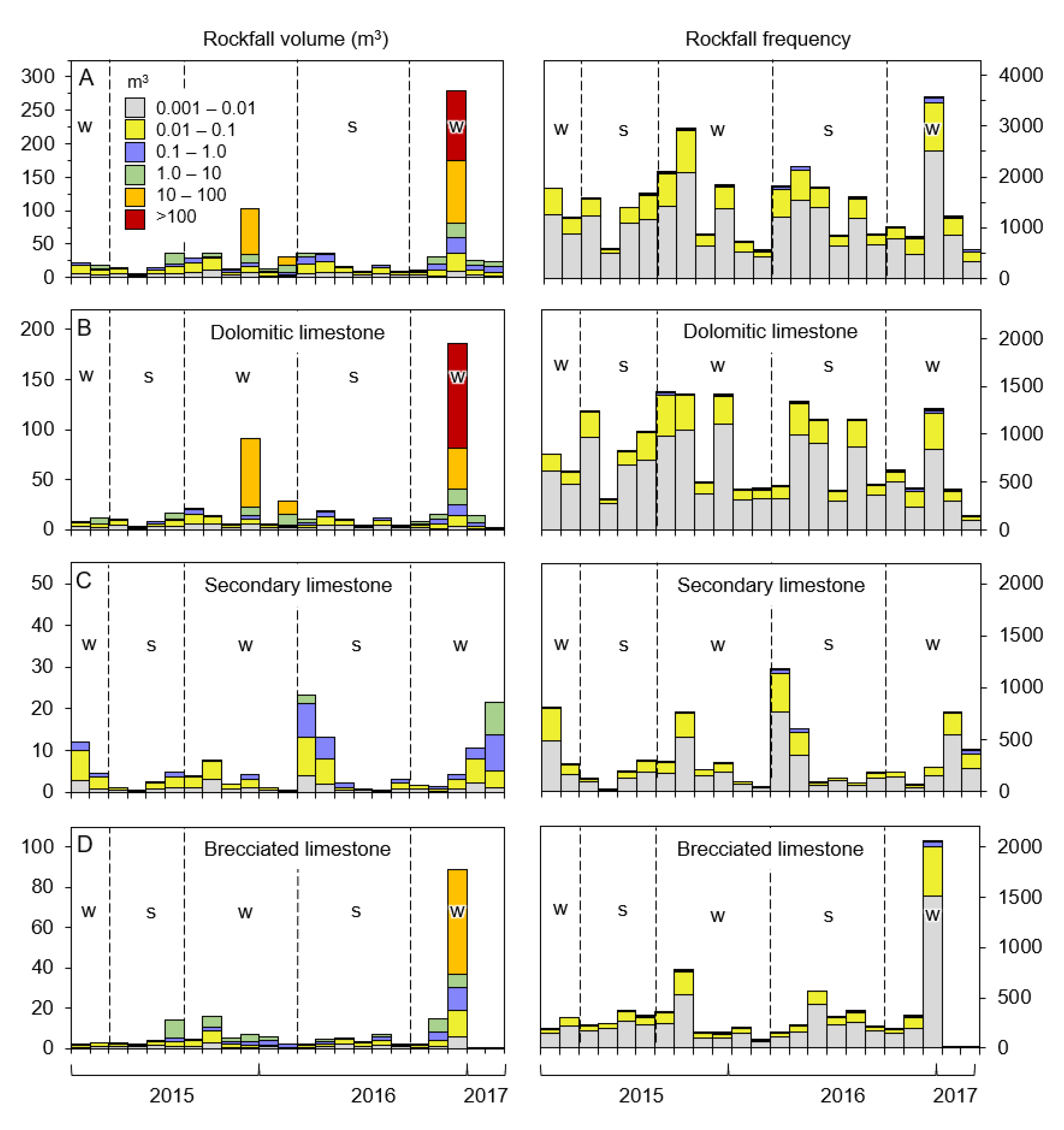
3.1. Summary of r = Rockfall Observations

A total of 30,428 rockfalls were detected over the ~2 year monitoring period, representing 835 m³ of material. Rockfall activity covered 12% of the cliff area, which equates to a local face refresh period (i.e., the time taken for rockfalls to occur across the whole cliff face) of ~17 years. By distributing our eroded volume across the cliff area, we determined the site-wide cliff retreat rate over our monitoring period as 0.032 m a⁻¹, amalgamating spatially and temporally constrained periods of enhanced activity. The mean retreat rate for each lithology was as follows: Dolomitic limestone 0.029 m a⁻¹; secondary limestone 0.079 m a⁻¹; brecciated limestone 0.010 m a⁻¹. These retreat rates are in the upper interquartile range of published erosion rates for other limestone cliffs worldwide (0.008–0.08 m a⁻¹; [45]). Notable large erosion scars included the loss of 69.3 m³ from a brecciated limestone outcrop at the cliff top between December 2015 and January 2016, and at the cliff toe (104.3 m³) in dolomitic limestone in the northern sector of the site between the January and February 2017 surveys (Figure 3). Both events generated localized erosion rates that exceed the site-wide mean by over an order of magnitude (max. 0.50 m a⁻¹); rarer large failures (≥0.1 m³) at this site contributed more to the overall volume of erosion at monthly-annual timescales than frequent smaller failures (0.001–0.1 m³), in line with similar observations from other rocky (e.g., [12,46,47]) and soft coast sites worldwide (e.g., [48,49,50]).

The mean rockfall depth was 0.142 m and the mean rockfall volume was 0.024 m³, and these metrics were broadly consistent between lithologies (e.g., mean volume range 0.020–0.027 m³, median range 0.005–0.006 m³). Rockfalls <0.01 and <0.1 m³ accounted for 71% and 98% of detected events, respectively, whilst rockfalls >0.1 m³ accounted for 89% of the total eroded volume. We additionally fitted a minimum bounding rectangle to each rockfall outline and extracted maximum width and height metrics. The mean width-to-height ratio of the rockfall inventory was 1.98 and the mean width-to-depth ratio was 2.20, implying that surficial as opposed to deep failures dominated, in line with observations from similar North Sea rocky coastlines [30]. Median facet length along the longest planar axis was 0.351, 0.164, and 0.236 m for the dolomitic, secondary, and brecciated limestones, respectively. By comparison, the median length of individual rockfall scars was 0.212, 0.207, and 0.214 m for respective lithologies, implying a structural control on rockfall dimensions for all lithologies, and for the brecciated limestone in particular.

The secondary limestone generated a greater eroded volume relative to its surface area (42% of total erosion across 20% of the cliff face), compared to the other lithologies (55% and 2.5% of total erosion across 71% and 9% of the cliff area for the dolomitic and brecciated limestones, respectively). Rockfall occurrence was much higher in the brecciated limestone (a mean of 12.3 rockfalls per m²) compared to other lithologies (means of 2.1 and 0.5 per m² for the dolomitic and secondary limestones, respectively), a distinction that is well-illustrated in Figure 4, where a clear lithological boundary in rockfall activity is apparent. The magnitude–frequency distribution of rockfalls, landslides, and rock avalanches determines the hazard posed by mass movements from a given slope. The magnitude and frequency of mass movements are commonly described using magnitude–frequency curves (e.g., [26]), to which an inverse power law is often fitted and used to estimate the recurrence interval of an event of a given size. The power law scaling exponent (α) describes the proportional contribution of increasingly small events. The cumulative magnitude–frequency relationship of our rockfall inventory fits an inverse power law distribution (Figure 5). We also derived lithology- and period-specific power laws, and later used period-specific α as a proxy for analyzing temporal variability in the proportional contribution of rockfall volumes, an approach that has successfully quantified storm effects in other coastal environments [51]. For our entire inventory, α = 2.19, whilst for the dolomitic, secondary, and brecciated limestones, α = 2.31, 2.25, and 2.19, respectively. The ‘rollover,’ or size fraction, below which the power law is not applicable was 0.007 m³ for the entire inventory, and in the range 0.004–0.014 m³ for lithology specific inventories.

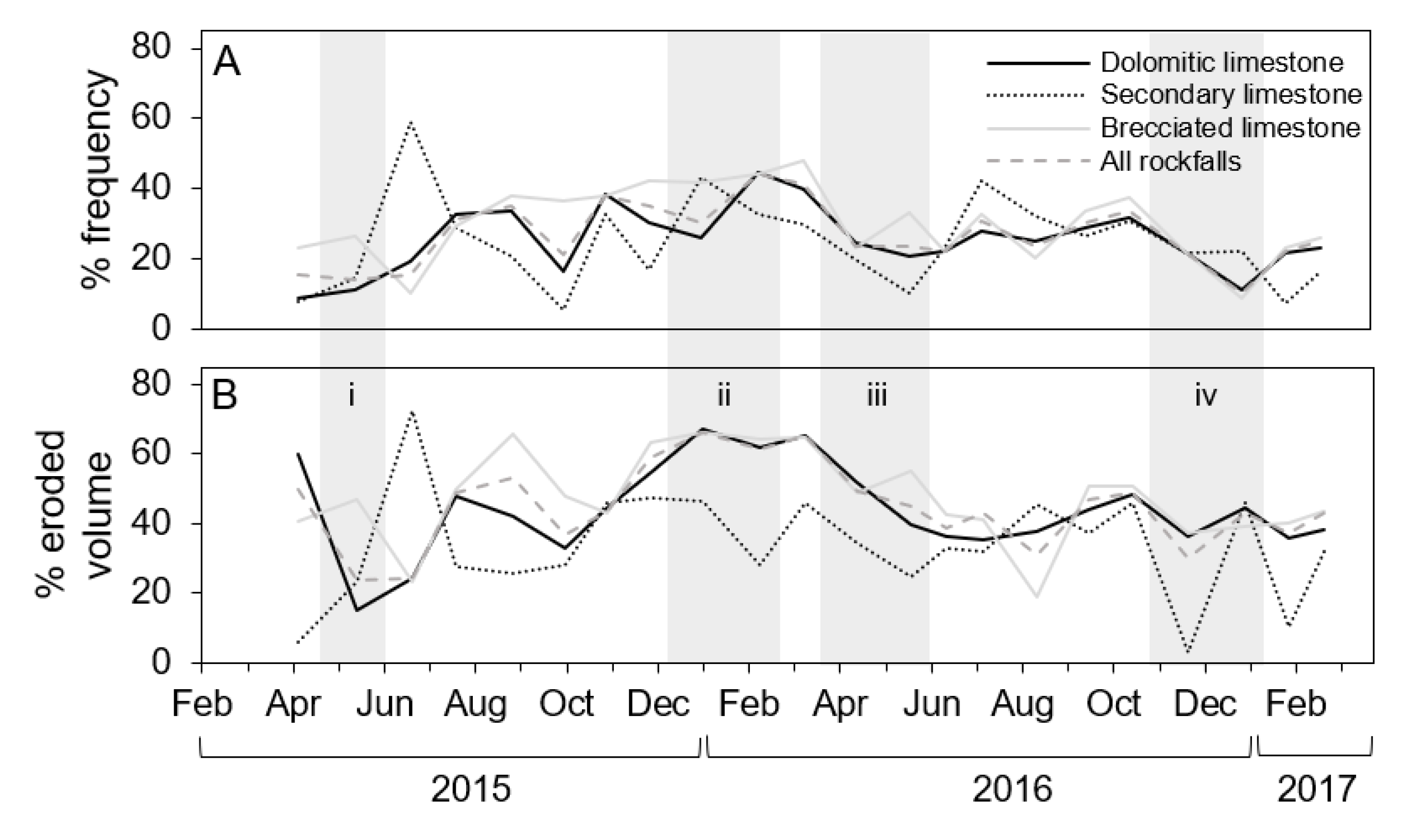
3.2. Spatiotemporal Patterns of Erosion Response

We observed complex spatiotemporal patterns of erosion (Figure 6) including regions that experience intense and short-lived (i.e., spanning a single monthly survey interval) periods of activity adjacent to areas with a more temporally consistent distribution of failure periodicity and volume. For instance, between 0.37 and 0.45 km, 96% of total erosion occurred in a 30 day monitoring window between December 2016 and January 2017 (Figure 6). At the extremes of the site (<0.05 and >0.5 km), summer and winter activity are more regularly distributed. Dominant periods of erosion in the dolomitic limestone broadly mirror those in the secondary limestone (Figure 6B,C), implying that these two lithologies generate rockfalls synchronously. Notable examples of this behavior occurred in the period from September to October 2016 and December 2016 to January 2017. Erosion that occurred in the period March–May 2016 accounted for >95% of all eroded volume in the dolomitic limestone between 0.33 and 0.35 km (Figure 6B). This period also accounted for a high proportion (40–95%) of eroded volume between 0.25 and 0.33 km distance in the adjacent brecciated limestone. Alternately, the period December 2015 to January 2016 was associated with enhanced activity in the brecciated limestone between 0.20 and 0.24 km (accounting for 23% of total erosion in this lithology) but did not stand out as a period of increased rockfall activity in the dolomitic or secondary limestone.

Lithology provides a clear spatial control on the occurrence of rockfalls (Figure 4). Events <0.1 m³ accounted for 33% and 38% of total eroded volume for the dolomitic and secondary limestones, respectively (Figure 7B,C), and 64% for the brecciated limestone, indicating that smaller rockfalls accounted for more erosion in this cliff material, an observation that is explained by the highly fragmented nature of the latter lithology. Aspects of commonality between lithologies included a tendency for larger-volume rockfalls (>10 m³) to occur in winter months (here, broadly defined as September–March) in the dolomitic and brecciated limestones (respectively Figure 7B,D), although our data do not span a timescale long enough to statistically resolve any seasonal control on rockfall generation. Differences between winter and summer rockfall activity become more evident as rockfalls increase in size: Across our entire inventory, winter activity accounted for 55%, 62%, 66%, 79%, and 100% of the eroded volume in successive size classes ranging from 0.001 to 100 m³ (with class boundaries at 0.01, 0.1, 1, 10, and 100 m³). This pattern was replicated in the rockfall volume data for the dolomitic limestone (winter volumetric contributions of 53%, 59% 71%, 84%, and 100% for respective volume classes), but was less clear for the secondary (60%, 61%, 52%, and 78%, with no rockfalls >10 m³) and brecciated limestones (58%, 68%, 75%, 69%, and 100%, with no rockfalls >100 m³). We also observed an increase in winter rockfall frequency relative to summer across all lithologies and volume classes: The mean winter rockfall contribution, by frequency, was 73% for the entire inventory (Figure 7A), and 77%, 63%, and 74% for the dolomitic, secondary, and brecciated limestones (Figure 7B–D), respectively.

3.3. Cliff Profile Analysis and Vertical Rockfall Zonation

The seasonal response of different lithologies was also evident in their 2D cliff and shore profiles, analyzed here through spatial variations in profile form and the height and timing of recorded failures (Figure 8). The brecciated limestone possessed the least variability in erosion rate with cliff height and exhibited the most consistent form (Figure 8). Further, erosion rates are generally lower in summer (mean 0.01 mm d⁻¹, max. 0.09 mm d⁻¹) and higher in winter (mean 0.04 mm d⁻¹, max. 0.9 mm d⁻¹). In the secondary limestone, we observed a progressive increase in erosion rate toward the base and top of the cliff (Figure 8); the mean erosion rate at the cliff center is <0.01 mm d⁻¹, increasing to 0.05 mm d⁻¹ at the cliff base, and >0.30 mm d⁻¹ at the cliff top. This pattern likely reflects the erosive influence of surface runoff from the cliff top and direct wave action at the cliff toe, respectively. However, over time, we would expect that enhanced erosion at the cliff toe would lead to destabilization of the overlying rock mass (e.g., [52]), leading to upward-propagating failure, and a corresponding positive vertical shift in the elevation at which peak erosion occurs. The short duration of our survey precludes such an observation, implying that this process likely operates across decadal timescales, as observed at other North Sea rocky coast sites [6].

Occasional winter peaks in erosion (max. 9 mm d⁻¹) exceeded the underlying base rates of change by over two orders of magnitude (mean 0.07 mm d⁻¹), and it is noteworthy that cliff profiles extending below the maximum offshore wave height in this lithology were characterized by cliff toe protrusion, contrasting those defended by boulder fields that were concave at the cliff base, where karstic collapse and wave processes may be more dominant. The winter signal in the dolomitic limestone (Figure 8B) also recorded peak rates of change (up to 7.5 mm d⁻¹ at 12 m elevation), although some winter surveys also recorded the lowest rates (<0.001 mm d⁻¹) at some elevations, suggesting a more spatially varied response over the monitoring period.

3.4. Event Superimposition

Previous studies have explored the significance of ‘progressive’ rockfall (abbreviated: PRF) evolution in driving rock cliff retreat in both coastal (e.g., [6,30]) and non-coastal settings [53,54,55]. Precursory rockfalls are commonly detected prior to the release of a larger mass, and, as such, represent a form of progressive rockfall. Rockfall scars can also act as an initiation point from which future rockfalls can originate, or progress; the latter has been shown to be a potentially significant driver of rocky coastline retreat [6]. Specifically, our terminology here serves to distinguish between ‘first time’ slope failures that do not appear to be spatially connected to other recorded slope instability events, and failures that can be shown to evolve from recent, existing rockfall scars that are detected within the wider monitoring period (i.e., PRFs). To explore the role that the latter plays in driving cliff retreat, we classified PRFs as those rockfalls whose outlines intersected a minimum of one other rockfall scar in any preceding differencing period and regard all other rockfalls as ‘new.’ We were thus required to remove the first differencing period from the analysis that follows. Additional methodological caveats included the following: (i) We only consider PRFs that have developed from new rockfall scars that were detected during our monitoring period; we do not consider spatial intersections with rockfall scars that pre-date our observation period, and (ii) we are unable to detect progressive scar growth, otherwise known as event superimposition, within a given differencing period. Where we refer to an ‘individual PRF,’ this may, in fact, represent multiple rockfalls, but the temporal resolution of our data preclude clarification. Due to these constraints, we are certain to underestimate the prevalence of PRF activity in our data, and so the relative frequency and volumetric contributions of PRF that we report below should be considered conservative estimates. Nevertheless, our data remain valuable for exploring PRF occurrence and potential environmental or lithological controls that operate over short (monthly) timescales.

We observed both precursory rockfall activity prior to larger failures and progressive scar enlargement following an initial detachment (Figure 9). PRFs accounted for 46.5% of all rockfalls by frequency but contributed 78.9% of the total eroded volume (Figure 10). When subdivided by lithology, we found that PRFs accounted for 44.1%, 41.1%, and 50.0% of rockfalls by frequency, and 81.5%, 47.1%, and 77.3% of the total eroded volume in the dolomitic, brecciated, and secondary limestone, respectively. In all lithologies the mean volume of a PRF exceeded that of a new rockfall by 0.03 m³, or the equivalent of a 0.3 m cube. The mean PRF volume in the brecciated limestone was smaller (0.02 m³) than other lithologies (0.04–0.06 m³), and the maximum volume for an individual PRF in this lithology was smaller (1.33 m³) than the maximum volume for a new rockfall (5.58 m³). By contrast, for the dolomitic and secondary limestone, the maximum PRF volume (104.30 and 36.35 m³, respectively) approached, or was greater than, an order of magnitude larger in volume compared to the largest new rockfalls. PRFs were equivalent in mean depth to new rockfalls (0.15 versus 0.14 m), and this finding was consistent between lithologies. The mean 3D surface area (0.15 m²) of a PRF was more than twice as large as a new rockfall (0.06 m²). This observation was consistent across lithologies, except for the brecciated limestone, where PRF surface area was, on average, 1.7 times larger than a new rockfall, compared to multipliers of 2.5 and 2.3 for the dolomitic and brecciated limestone, respectively. Combined, our findings imply that PRFs contributed less relative volume overall for the brecciated limestone than for the other two lithologies. We found no discernible variation in PRF frequency distribution according to height on the cliff face. The power-law scaling exponents of our PRF and ‘new’ rockfall inventories were 2.07 and 2.50, respectively, reflecting the larger volume of individual PRFs.

4. Discussion

Our results demonstrate the complexity of rock cliff erosion responses spatially and over time. We have developed a detailed rockfall inventory that has allowed the exploration of connections between, and controls on, apparently disparate and episodic geomorphic behavior, which we elaborate on below with respect to their implications for wider studies of rock slope environments.

4.1. Rockfall Development

Summary rockfall descriptors (e.g., mean depth, volume) were broadly consistent between lithologies but masked varied spatiotemporal patterns of activity that reveal the complex interplay of lithological structure and competence, erosional conditioning and environmental forcing, and possible modulation by foreshore geomorphology and in situ cliff conditions. Rockfall activity was characterized by frequent, small failures that can be typical of rock slope behavior in both coastal (e.g., [6,12,22,23,26,32]) and many non-coastal settings [21,24], but the total eroded volume was dominated by large events that occurred infrequently; rockfalls >1 and >10 m³ occurred approximately every 2 and 9.5 months, respectively, and affected all lithologies (Figure 7). We note an absence of large (>10 m³) failures in the secondary limestone, perhaps because the return period for such events is longer than our two-year monitoring period. Alternatively, joint spacing has previously been shown to be a controlling factor of rockfall size distribution (e.g., [6,56,57]) and, thus, the smaller median facet length of the secondary limestone (0.164 m) relative to the dolomitic limestone (0.351 m) could result in a higher propensity for failure to occur as smaller events instead of longer-term stress accumulation within rock bridges as found in rocks with wider joint spacing [29]. This control was even stronger in the highly fragmented brecciated limestone, which lacks the structural coherence observed in the other lithologies (Figure 2B); individual clasts are contained within a finer-grained matrix that has a low resistance to weathering. These findings demonstrate that layer-specific rockfall inventories are required to better understand rock slope responses. Additionally, in cliff sections that contained dolomitic limestone overlain by brecciated limestone, significant changes occurred first in the weaker breccia, and then in the more competent dolomite. This sequence reverses patterns of spatially constrained upward failure evolution, recorded within rock masses containing less geotechnically varied layers [6], highlighting the importance for future studies to account for the ordering of and interaction between the lithological boundaries in the assessment of the timing and nature of rockfall risks.

Event superimposition is a significant control on erosion at our site; PRFs accounted for ~80% of total eroded volume but accounted for less than half of all erosion scars. PRFs were the dominant mechanism of cliff face retreat in the dolomitic and secondary limestones over annual timescales, but did not exert an overriding control on the erosional signal in the brecciated limestone. Further, the mean volume of PRFs in the brecciated limestone was smaller than other lithologies, implying that lithological structure is a limiting factor on the relative volumetric contribution of progressive failures in this lithology. By contrast, PRFs in the dolomitic and secondary limestones were larger than ‘new,’ or first-time, failures, perhaps as a function of the coalescence of contiguous failure scars, and the bridging of proximal scars, thereby producing larger rockfalls [6,58]. The spatial connection between rockfalls, and the associated generation of ‘hotspots’ of activity, may reflect de Vilder et al.’s [58] theory of localized progressive failure related to stress release and rock bridge failure, working to separate cliff failures from triggering events [30]. The implication for the resultant rockfall hazard is that the probabilities of occurrence are not evenly distributed spatially across the rock face and there may be detectable times of heightened activity in specific locations.

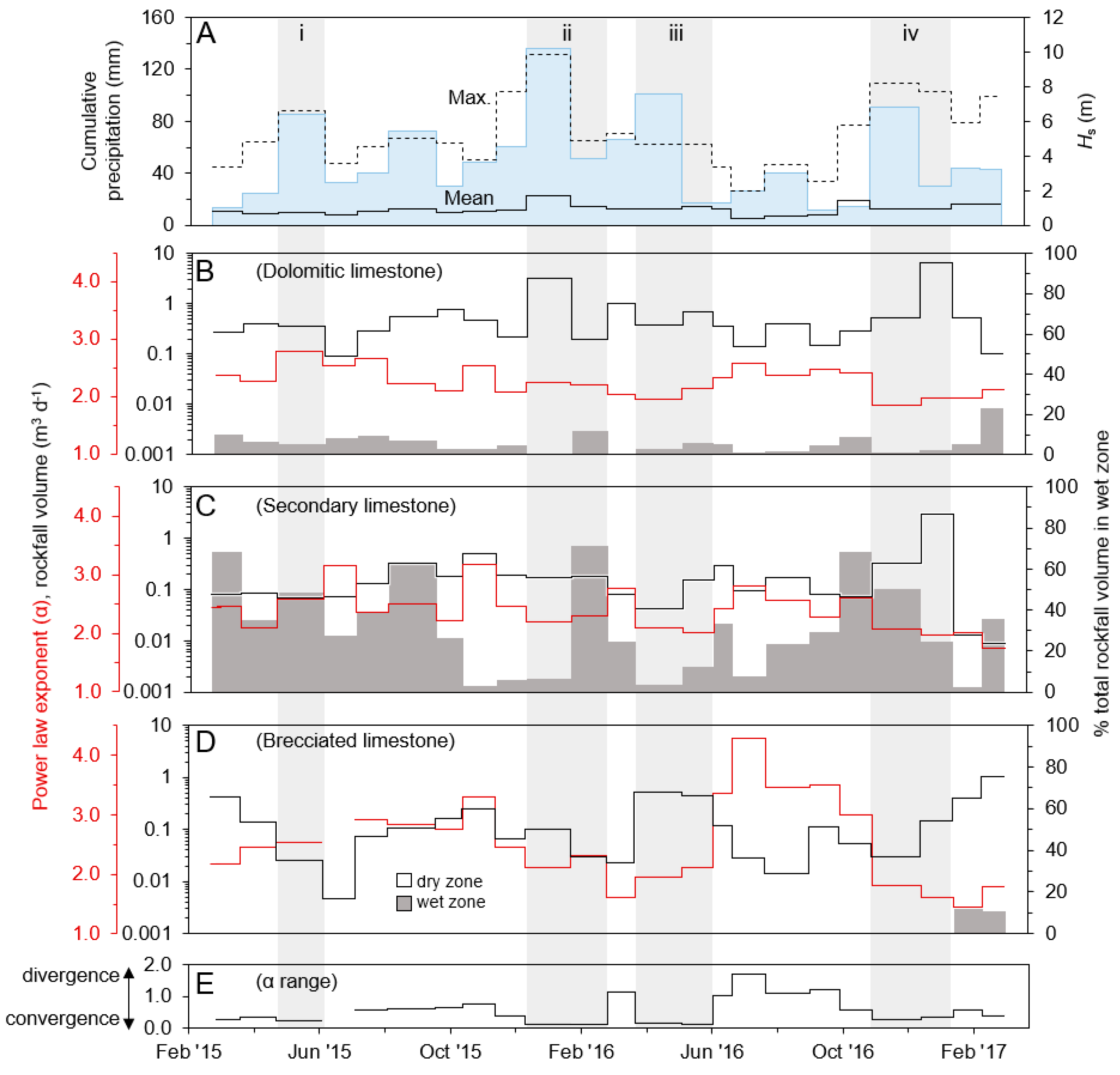
4.2. Links to Environmental Drivers

Erosion rates during winter months are generally higher than those in summer months, a finding that is also consistent across the cliff height in all lithologies (Figure 8B). However, due to the short time period that our data span (geologically speaking), we could not statistically test for a seasonal control on erosion rates. Similarly, because we did not undertake wave transformation modeling, we cannot make robust statistical inferences between key marine controls and erosion response. However, our data show that detectable increases in rockfall volumes within the monitored period coincided with individual winter storm events and associated short-term increases in precipitation and wave activity. Rather than an assumed sustained increase in erosion rates during winter months, we observed direct event-specific responses, in accordance with observations in other rock coast environments [59]. Heightened rockfall activity in winter has been noted in other rock slope environments [24], but our data evidence a potential departure from episodic and temporally disconnected perceptions of rock failure. However, this hypothesis requires further testing through analysis of rockfall inventories captured over a longer (i.e., decadal) time period, and in different rock cliff environments.

We define a ‘stormy period’ as one during which storms were identified and named by the UK Meteorological Office [60] and affected northern England, or, for periods prior to November 2015 (when the UK first adopted a standardized storm naming convention), periods where the cumulative precipitation and maximum significant wave height exceeded 80 mm and 4 m, respectively, characteristics shared by periods in which named storms occurred. We observed varying degrees of spatiotemporal connectivity between periods where storms occurred, and rockfall activity. For example, an increased proportion of erosion occurred in the ‘wet’ zone in the secondary limestone in the period immediately following a large storm in December 2015 (Figure 11), but this did not produce an overall increase in eroded volume. Previous work has found statistically significant positive relationships between wind velocity and various rockfall inventory descriptors [10] and demonstrated that breaking wave energy at the cliff toe can be delivered to the cliff top [61]. At Marsden Bay, this effect might be particularly efficient at triggering rockfalls at the cliff top, including large failures (Figure 3B), but in situ seismic monitoring data are required to explore this effect in more detail (e.g., [62]).

We observed a distinct storm signal in the rockfall distributions that pervades all lithologies, which suggests a uniform cliff system response. The scaling law exponent of a power law describes the proportional contribution of specific sizes of events [26,63]. Storm occurrence coincides with convergence in the power law exponents (Figure 11E), implying that high-energy events can generate synchronous behavior across all lithological units. At Marsden Bay, exponent convergence manifested as a consistent decrease in the scaling exponent, implying a shift toward the increasing prevalence of larger-volume rockfalls during stormy periods (e.g., [64]). Fewer rockfalls were produced from the secondary limestone (n = 10¹–10² per differencing period) than the dolomitic or brecciated limestones (n = 10²–10³), but the relative size distribution remained consistent between differencing periods for each lithology, and was comparable to the size distribution of the entire ~2 year inventory for each lithology, providing confidence that exponent convergence was controlled by short-lived shifts in the size distribution and was not a product of inadequate rockfall inventory size. The convergence of power law scaling exponents has been used to quantify storm-impacts in coastal dune cliff systems [65] and, here, it has proven an effective approach for understanding complex rock cliff behavior, specifically short-term synchronicity in erosion responses. Questions remain over whether a storm-related erosion signature is the same for all events, reflective of the magnitude of the storm, or altered by the in situ conditions of the cliff.

There is a historical disconnect between studies that focus on either shore platform or rock cliff processes [66], but, here, we show enhanced rockfall activity at sections not protected by boulder fields and, hence, subjected to the highest cumulative tidal cliff toe inundation over the monitoring period (Figure 1C). Foreshore composition and characteristics are often investigated separately from cliff process studies, but, here, we show how holistic foreshore-cliff analysis aids the interpretation of the superimposition of erosion dynamics at rocky coasts. The focusing of marine energy related to incised channels in shore platform (Figure 1A), or the dissipative effect of platform material or structures, exerts key controls on cliff toe exposure and results in local divergence from classic models of undercutting and cantilever collapse [50]. Outside of periods of scaling exponent convergence (Figure 11E), we hypothesize that the erosion response of the secondary limestone is largely marine-driven, and certainly for small- (<0.1 m³) and mid-range (0.1–1.0 m³) failures. The volumetric contribution of PRFs in both the dolomitic limestone and the secondary limestone also increases during stormy periods (Figure 10B). However, we do not observe this behavior in the fragile brecciated limestone; direct transfer of marine energy to this lithology is likely to be limited because much of the brecciated material is protected from wave action by extensive boulder fields and discontinuous sections of shore platform at the cliff base (Figure 1 and Figure 2B).

4.3. Implications for Coastal Monitoring and Geohazard Assessment

Whilst high-resolution analyses of rockfall inventories are typically limited in temporal extent, they can provide important information to better understand rock cliff erosion processes and their drivers, and ultimately to mitigate the impacts of uncertainty in failure dynamics. A number of aspects of this work contribute to an improved understanding of coastal cliff geohazards, both locally and more generally. On a basic level, high-quality rockfall data have enabled a re-evaluation of the conservatively high rates of cliff erosion previously relied upon for decision-making at this site, and which are derived from potentially error-prone historic cliff line retreat mapping; our new high-resolution dataset provides a wealth of quantitative data on the erosion dynamics of specific rock types, enabling complex geomorphic signals to be identified and analyzed. We found that the brecciated limestone generated more frequent rockfalls than the other two lithologies, and, temporally speaking, rockfalls from this lithology might be considered a more persistent hazard. By contrast, rockfall activity in the dolomitic and secondary limestones was more sensitive to environmental forcing. Rapid, possibly instantaneous, step-back of the entire cliff face occurred at a frequency greater than 2 years, whilst rockfalls >1 and 10 m³ occurred every ~2 and ~9.5 months, respectively, and this applied to all lithologies. The true risk of rockfalls results from both the detachment of an initial rockfall volume, followed by the potential for failure propagation across a slope and the generation of additional rockfalls. We found that PRFs accounted for ~80% of the total eroded volume, but occurred less frequently than initial, or ‘new,’ failures. We also found that the volumetric contribution of PRFs in the dolomitic and secondary limestones increased during stormy periods. These data show more widely that knowledge of short-term patterns and the connectivity of rockfall events is potentially vital for effective coastal management of rockfall risk, given that individual PRFs were also larger in volume than ‘first-time’ detachments.

Ultimately, the timescales required for coastal management span from those applicable to hazard mitigation (days-years) to strategic planning (≥decades), but the key challenge remains in dealing with uncertainty in cliff geomorphic behavior. Comprehensive risk assessment for slope rockfall hazards requires knowledge of rockfall geometries, triggers (intrinsic and extrinsic), failure dynamics and propagation, and timing, the latter of which is the more difficult to elucidate [30,67]. Similarly, the uncertainty surrounding how cliffs will change, how fast, and over what timeframes, and in response to which drivers, has direct impacts on costly decisions such as whether to relocate an asset, when and how to remediate sea defenses, and advising coastal users of higher-risk periods or locations. To this end, establishing links between failure volume and periodicity, for example, through the application of magnitude–frequency power laws, remains invaluable, but previous studies (e.g., [67]) failed to link the power law slope or scaling exponents with environmental conditions, limiting their utility for practical application. Further work is required to explore whether temporal convergence–divergence in a rockfall volume distribution during stormy periods identified here can be statistically linked to extrinsic environmental drivers and is a significant avenue for future research to explore. From a coastal management perspective, such a finding would be significant; for sites where cliffs are composed of a range of lithologies, it may be possible for practitioners to use such relationships in combination with, for example, marine forecasts, or real-time offshore wave buoy data and wave transformation modeling to infer site- or layer-specific, short-term temporal sequencing of the rockfall size distribution, and associated short-term hazard increases that threaten coastal users, assets, or infrastructure.

5. Conclusions

We have presented an analysis of a rockfall inventory acquired through high-resolution topographic change detection applied to a section of limestone coastal rocky cliff in northeast England. The work highlights the value of high-resolution surveys in constraining the geometry, failure mechanisms, and drivers of erosion of rocky coastal cliffs, how these vary in space and time, and the implications for hazard assessment. Our data demonstrate the importance of lithological succession where layer competence varies significantly, potentially controlling the nature and location of rockfall occurrence and processes driving longer-term cliff evolution. Progressive rockfall evolution is shown here to be significant in driving eroded volume, if not frequency, leading to a spatially concentrated rockfall hazard. However, the relative importance of progressive failures remains lithology-dependent: The brecciated limestone, an exceptionally weak and fragmented lithology, exhibited a short-term erosional regime more in line with the dominance of intrinsic rather than extrinsic controls on rockfall generation. We present an analysis of rockfall distributions that signals a coherent erosion response between certain rock types to storm activity, which manifests as temporary convergence of the magnitude–frequency power law scaling exponent and an associated short-term shift toward larger failure volumes during stormy periods. This coherent response was distinct from background variations in erosion activity otherwise associated with foreshore properties and other system controls. The ability to summarize a complex geomorphic response within a single summary metric like a scaling exponent has wide ranging potential applications for understanding and ultimately predicting geomorphic responses. From a hazard management perspective, future work should focus on linking extrinsic erosion drivers to statistically modeled rockfall responses in this way in order to develop a new predictive tool for quantifying temporal convergence in rockfall dynamics over timescales that are relevant for hazard assessment and mitigation.

References

1. Selby, M.J. Hillslope Materials and Processes; Oxford University Press: New York, NY, USA, 1982. [Google Scholar]
2. Dorren, L.K.A. A Review of Rockfall Mechanics and Modelling Approaches. Prog. Phys. Geogr. 2003, 27, 69–87. [Google Scholar] [CrossRef]
3. Trenhaile, A.S. Rock Coasts, with Particular Emphasis on Shore Platforms. Geomorphology 2002, 48, 7–22. [Google Scholar] [CrossRef]
4. Gilham, J.; Barlow, J.; Moore, R. Marine Control over Negative Power Law Scaling of Mass Wasting Events in Chalk Sea Cliffs with Implications for Future Recession under the UKCP09 Medium Emission Scenario. Earth Surf. Process. Landf. 2018, 43. [Google Scholar] [CrossRef]
5. Emery, K.O.; Kuhn, G.G. Sea Cliffs: Their Processes, Profiles, and Classification. Geol. Soc. Am. Bull. 1982, 93, 644–654. [Google Scholar] [CrossRef]
6. Rosser, N.J.; Brain, M.J.; Petley, D.N.; Lim, M.; Norman, E.C. Coastline Retreat via Progressive Failure of Rocky Coastal Cliffs. Geology 2013, 41, 939–942. [Google Scholar] [CrossRef] [Green Version]
7. Bezerra, M.M.; Moura, D.; Ferreira, O.; Taborda, R. Influence of Wave Action and Lithology on Sea Cliff Mass Movements in Central Algarve Coast, Portugal. J. Coast. Res. 2011, 27, 162–171. [Google Scholar] [CrossRef]
8. Limber, P.W.; Murray, A.B. Beach and Sea-Cliff Dynamics as a Driver of Long-Term Rocky Coastline Evolution and Stability. Geology 2011, 39, 1147–1150. [Google Scholar] [CrossRef] [Green Version]
9. Swirad, Z.M.; Rosser, N.J.; Brain, M.J.; Vann Jones, E.C. What Controls the Geometry of Rocky Coasts at the Local Scale? J. Coast. Res. 2016, 612–616. [Google Scholar] [CrossRef]
10. Vann Jones, E.C.; Rosser, N.J.; Brain, M.J.; Petley, D.N. Quantifying the Environmental Controls on Erosion of a Hard Rock Cliff. Mar. Geol. 2015, 363, 230–242. [Google Scholar] [CrossRef] [Green Version]
11. Naylor, L.A.; Spencer, T.; Lane, S.N.; Darby, S.E.; Milligan, F.J.; Macklin, M.G.; Möller, I. Stormy Geomorphology: Geomorphic Contributions in an Age of Climate Extremes. Earth Surf. Process. Landf. 2017, 42, 166–190. [Google Scholar] [CrossRef]
12. Lim, M.; Rosser, N.J.; Allison, R.J.; Petley, D.N. Erosional Processes in the Hard Rock Coastal Cliffs at Staithes, North Yorkshire. Geomorphology 2010, 114, 12–21. [Google Scholar] [CrossRef]
13. Naylor, L.A.; Stephenson, W.J.; Trenhaile, A.S. Rock Coast Geomorphology: Recent Advances and Future Research Directions. Geomorphology 2010, 114, 3–11. [Google Scholar] [CrossRef]
14. Kennedy, D.M.; Coombes, M.A.; Mottershead, D.N. The Temporal and Spatial Scales of Rocky Coast Geomorphology: A Commentary. Earth Surf. Process. Landf. 2017, 42, 1597–1600. [Google Scholar] [CrossRef]
15. Lim, M.; Petley, D.N.; Rosser, N.J.; Allison, R.J.; Long, A.J.; Pybus, D. Combined Digital Photogrammetry and Time-of-Flight Laser Scanning for Monitoring Cliff Evolution. Photogramm. Rec. 2005, 20, 109–129. [Google Scholar] [CrossRef]
16. Dewez, T.J.B.; Rohmer, J.; Regard, V.; Cnudde, C. Probabilistic Coastal Cliff Collapse Hazard from Repeated Terrestrial Laser Surveys: Case Study from Mesnil Val (Normandy, northern France). J. Coast. Res. 2013, 65, 702–707. [Google Scholar] [CrossRef]
17. Brunier, G.; Fleury, J.; Anthony, E.J.; Gardel, A.; Dussouillez, P. Close-range airborne Structure-from-Motion photogrammetry for high-resolution beach morphometric surveys: Examples from an embayed rotating beach. Geomorphology 2016, 261, 76–88. [Google Scholar] [CrossRef]
18. Esposito, G.; Salvini, R.; Matano, F.; Sacchi, M.; Danzi, M.; Somma, R.; Troise, C. Multitemporal Monitoring of a Coastal Landslide through SfM-Derived Point Cloud Comparison. Photogramm. Rec. 2017, 32, 459–479. [Google Scholar] [CrossRef] [Green Version]
19. Matano, F.; Pignaloso, A.; Marino, E.; Esposito, G.; Caccavale, M.; Caputo, T.; Sacchi, M.; Somma, R.; Troise, C.; De Natale, G. Laser Scanning Application for Geostructural Analysis of Tuffaceous Coastal Cliffs: The Case of Punta Epitaffio, Pozzuoli Bay, Italy. Eur. J. Remote Sens. 2015, 48, 615–637. [Google Scholar] [CrossRef] [Green Version]
20. Young, A.P. Decadal-Scale Coastal Cliff Retreat in Southern and Central California. Geomorphology 2018, 300, 164–175. [Google Scholar] [CrossRef]
21. Abellán, A.; Calvet, J.; Vilaplana, J.M.; Blanchard, J. Detection and Spatial Prediction of Rockfalls by Means of Terrestrial Laser Scanner Monitoring. Geomorphology 2010, 119, 162–171. [Google Scholar] [CrossRef]
22. Teixeira, S.B. Slope Mass Movements on Rocky Sea-Cliffs: A Power-Law Distributed Natural Hazard on the Barlavento Coast, Algarve, Portugal. Cont. Shelf Res. 2006, 26, 1077–1091. [Google Scholar] [CrossRef]
23. Marques, F.M.S.F. Magnitude-Frequency of Sea Cliff Instabilities. Nat. Hazards Earth Syst. Sci. 2008, 8, 1161–1171. [Google Scholar] [CrossRef] [Green Version]
24. van Veen, M.; Hutchinson, D.J.; Kromer, R.; Lato, M.; Edwards, T. Effects of Sampling Interval on the Frequency-Magnitude Relationship of Rockfalls Detected from Terrestrial Laser Scanning Using Semi-Automated Methods. Landslides 2017, 9, 1–14. [Google Scholar] [CrossRef]
25. Westoby, M.J.; Lim, M.; Hogg, M.; Pound, M.J.; Dunlop, L.; Woodward, J. Cost-Effective Erosion Monitoring of Coastal Cliffs. Coast. Eng. 2018, 138, 152–164. [Google Scholar] [CrossRef]
26. Williams, J.G.; Rosser, N.J.; Hardy, R.J.; Brain, M.J.; Afana, A.A. Optimising 4D Approaches to Surface Change Detection: Improving Understanding of Rockfall Magnitude-Frequency. Earth Surf. Dyn. 2018, 6, 101–119. [Google Scholar] [CrossRef] [Green Version]
27. Rohmer, J.; Dewez, T. Analysing the Spatial Patterns of Erosion Scars Using Point Process Theory at the Coastal Chalk Cliff of Mesnil-Val, Normandy, Northern France. Nat. Hazards Earth Syst. Sci. 2015, 15, 349–362. [Google Scholar] [CrossRef] [Green Version]
28. Collins, B.D.; Stock, G.M. Rockfall Triggering by Cyclic Thermal Stressing of Exfoliation Fractures. Nat. Geosci. 2016, 9, 395–400. [Google Scholar] [CrossRef]
29. Brain, M.J.; Rosser, N.J.; Norman, E.C.; Petley, D.N. Are Microseismic Ground Displacements a Significant Geomorphic Agent? Geomorphology 2014, 207, 161–173. [Google Scholar] [CrossRef] [Green Version]
30. Rosser, N.; Lim, M.; Petley, D.; Dunning, S.; Allison, R. Patterns of Precursory Rockfall Prior to Slope Failure. J. Geophys. Res. 2007, 112, F04014. [Google Scholar] [CrossRef]
31. Esposito, G.; Matano, F.; Sacchi, M.; Salvini, R. Mechanisms and Frequency-Size Statistics of Failures Characterizing a Coastal Cliff Partially Protected from Wave Erosive Action. Rend. Lincei. Sci. Fis. E Nat. 2020, 31, 337–351. [Google Scholar] [CrossRef]
32. Benjamin, J.; Rosser, N.J.; Brain, M.J. Emergent Characteristics of Rockfall Inventories Captured at a Regional Scale. Earth Surf. Process. Landf. 2020, in press. [Google Scholar] [CrossRef]
33. Smith, D.B.; Francis, E.A.; Calver, M.A.; Gaunt, G.D.; Pattison, J.; Edwards, A.H.; Harrison, R.K. Geology of the Country between Durham and West Hartlepool (Explanation of Sheet 27, New Series). Memoirs of the Geological Survey of Great Britain 1967, England and Wales, Ref. DF027B. Available online: https://www.bgs.ac.uk/data/publications/pubs.cfc?method=viewRecord&publnId=19864698 (accessed on 5 August 2020).
34. Cooper, A.H.; Whitbread, K.; Irving, A.M. Environment Agency: Durham Permian Sections. Environmental Agency Internal Report 2007, CR/07/117. Available online: http://nora.nerc.ac.uk/id/eprint/516223/1/CR07117N.pdf (accessed on 5 August 2020).
35. South Tyneside Council. Cell 1 Regional Coastal Monitoring Programme Analytical Report 12: ‘Full Measures’ Survey 2019. Available online: http://www.northeastcoastalobservatory.org.uk/data/Reports/ (accessed on 5 August 2020).
36. Haskoning, R. Shoreline Management Plan 2: River Tyne to Flamborough Head. Report 9P0184/R/nl/PBor. 2007. Available online: http://www.northeastcoastalobservatory.org.uk/data/Reports/ (accessed on 5 August 2020).
37. Massiot, C.; Nicol, A.; Townend, J.; McNamara, D.; Garcia-Sellés, D.; Conway, C.; Archibald, G. Quantitative Geometric Description of Fracture Systems in an Andesite Lava Flow Using Terrestrial Laser Scanner Data. J. Volcanol. Geotherm. Res. 2017, 341, 315–331. [Google Scholar] [CrossRef] [Green Version]
38. Dewez, T.; Girardeau-Montaut, D.; Allanic, C.; Rohmer, J. FACETS: A Cloudcompare Plugin to Extract Geological Planes from Unstructured 3D Point Clouds. Int. Arch. Photogramm. Remote Sens. Spat. Inf. Sci. Xli-B5 2016, 799–804. [Google Scholar] [CrossRef]
39. Westoby, M.J.; Brasington, J.; Glasser, N.F.; Hambrey, M.J.; Reynolds, J.M. ‘Structure-from-Motion’ Photogrammetry: A Low-Cost, Effective Tool for Geoscience Applications. Geomorphology 2012, 179, 300–314. [Google Scholar] [CrossRef] [Green Version]
40. Carbonneau, P.E.; Dietrich, J.T. Cost-Effective Non-Metric Photogrammetry from Consumer-Grade Suas: Implications for Direct Georeferencing of Structure from Motion Photogrammetry. Earth Surf. Process. Landf. 2017, 42, 473–486. [Google Scholar] [CrossRef] [Green Version]
41. Rosnell, T.; Honkavaara, E. Point Cloud Generation from Aerial Image Data Acquired by a Quadrocopter Type Micro Unmanned Aerial Vehicle and a Digital Still Camera. Sensors 2012, 12, 453–480. [Google Scholar] [CrossRef] [Green Version]
42. James, M.R.; Robson, S. Mitigating Systematic Error in Topographic Models Derived from Uav and Ground-Based Image Networks. Earth Surf. Process. Landf. 2014, 39, 1413–1420. [Google Scholar] [CrossRef] [Green Version]
43. Lim, M.; Strzelecki, M.C.; Kasprzak, M.; Swirad, Z.M.; Webster, C.; Woodward, J.; Gjelten, H. Arctic Rock Coast Responses under a Changing Climate. Remote Sens. Environ. 2020, 236, 111500. [Google Scholar] [CrossRef]
44. Krautblatter, M.; Funk, D.; Günzel, K. Why Permafrost Rocks Become Unstable: A Rock-Ice-Mechanical Model in Time and Space. Earth Surf. Process. Landf. 2013, 38, 876–887. [Google Scholar] [CrossRef] [Green Version]
45. Prémaillon, M.; Regard, V.; Dewez, T.J.; Auda, Y. GlobR2C2 (Global Recession Rates of Coastal Cliffs): A Global Relationship Database to Investigate Coastal Rocky Cliff Erosion Rate Variations. Earth Surf. Dyn. 2018, 6, 651–668. [Google Scholar] [CrossRef] [Green Version]
46. Barlow, J.; Gilham, J.; Cofrã, I. Kinematic Analysis of Sea Cliff Stability Using UAV Photogrammetry. Int. J. Remote Sens. 2017, 38, 2464–2479. [Google Scholar] [CrossRef]
47. Letortu, P.; Costa, S.; Maquaire, O.; Davidson, R. Marine and Subaerial Controls of Coastal Chalk Cliff Erosion in Normandy (France) Based on a 7-Year Laser Scanner Monitoring. Geomorphology 2019, 335, 76–91. [Google Scholar] [CrossRef]
48. Hall, J.W.; Meadowcroft, I.C.; Lee, E.M.; van Gelder, P.H.A.J.M. Stochastic Simulation of Episodic Soft Coastal Cliff Recession. Coast. Eng. 2002, 46, 159–174. [Google Scholar] [CrossRef]
49. Furlani, S.; Devoto, S.; Biolchi, S.; Cucchi, F. Factors Triggering Sea Cliff Instability along the Slovenian Coasts. J. Coast. Res. 2011, 387–393. [Google Scholar] [CrossRef]
50. Johnstone, E.; Raymond, J.; Olsen, M.J.; Driscoll, N. Morphological Expressions of Coastal Cliff Erosion Processes in San Diego County. J. Coast. Res. 2016, 76, 174–184. [Google Scholar] [CrossRef] [Green Version]
51. Lim, M.; Dunning, S.A.; Burke, M.; King, H.; King, N. Quantification and Implications of Change in Organic Carbon Bearing Coastal Dune Cliffs: A Multiscale Analysis from the Northumberland Coast, UK. Remote Sens. Environ. 2015, 163, 1–12. [Google Scholar] [CrossRef] [Green Version]
52. Kogure, T.; Matsukura, Y. Critical Notch Depths for Failure of Coastal Limestone Cliffs: Case Study at Kuro-shima Island, Okinawa, Japan. Earth Surf. Process. Landf. 2010, 35, 1044–1056. [Google Scholar] [CrossRef]
53. Stock, G.M.; Martel, S.J.; Collins, B.D.; Harp, E.L. Progressive Failure of Sheet Rock Slopes: The 2009-2010 Rhombus Wall rock falls in Yosemite Valley, California, USA. Earth Surf. Process. Landf. 2012, 37, 546–561. [Google Scholar] [CrossRef]
54. Kromer, R.A.; Hutchinson, D.J.; Lato, M.J.; Gauthier, D.; Edwards, T. Identifying Rock Slope Failure Precursors Using LIDAR for Transportation Corridor Hazard Management. Eng. Geol. 2015, 195, 93–103. [Google Scholar] [CrossRef]
55. Royán, M.J.; Abellán, A.; Vilaplana, J.M. Progressive Failure Leading to the 3 December 2013 Rockfall at Puigcercós Scarp (Catalonia, Spain). Landslides 2015, 12, 585–595. [Google Scholar] [CrossRef]
56. Matsuoka, N.; Sakai, H. Rockfall Activity from an Alpine Cliff during Thawing Periods. Geomorphology 1999, 23, 309–328. (accessed on 5 August 2020). [Google Scholar] [CrossRef]
57. Sass, O.; Krautblatter, M. Debris Flow-Dominated and Rockfall-Dominated Talus Slopes: Genetic Models Derived from Gpr Measurements. Geomorphology 2007, 86, 176–192. [Google Scholar] [CrossRef]
58. de Vilder, S.J.; Rosser, N.J.; Brain, M.J. Forensic Analysis of Rockfall Scars. Geomorphology 2017, 295, 202–214. [Google Scholar] [CrossRef] [Green Version]
59. Naylor, L.A.; Stephenson, W.J.; Smith, H.C.M.; Way, O.; Mendelssohn, J.; Cowley, A. Geomorphological Control on Boulder Transport and Coastal Erosion before, during and after an Extreme Extra-Tropical Cyclone. Earth Surf. Process. Landf. 2016, 41, 685–700. [Google Scholar] [CrossRef] [Green Version]
60. The Meteorological Office (Met Office), UK Storm Centre. 2019. Available online: https://www.metoffice.gov.uk/weather/warnings-and-advice/uk-storm-centre/index (accessed on 5 August 2020).
61. Young, A.P. Observations of Coastal Cliff Base Waves, Sand Levels, and Cliff Top Shaking. Earth Surf. Process. Landf. 2016, 41, 1564–1573. [Google Scholar] [CrossRef] [Green Version]
62. Vann Jones, E.C.; Rosser, N.J.; Brain, M.J. Alongshore Variability in Wave Energy Transfer to Coastal Cliffs. Geomorphology 2018, 322, 1–14. [Google Scholar] [CrossRef]
63. Stark, C.P.; Hovius, N. The Characterization of Landslide Size Distributions. Geophysical Res. Lett. 2001, 28, 1091–1094. [Google Scholar] [CrossRef]
64. Gilham, J.; Barlow, J.; Moore, R. Detection and Analysis of Mass Wasting Events in Chalk Sea Cliffs Using UAV Photogrammetry. Eng. Geol. 2019, 250, 101–112. [Google Scholar] [CrossRef] [Green Version]
65. Stephenson, W.J.; Kirk, R.M.; Kennedy, D.M.; Finlayson, B.L.; Chen, Z. Long Term Shore Platform Surface Lowering Rates: Revisiting Gill and Lang after 32 Years. Mar. Geol. 2012, 299, 90–95. [Google Scholar] [CrossRef]
66. Dussauge-Peisser, C.; Helmstetter, A.; Grasso, J.R.; Hantz, D.; Desvarreaux, P.; Jeannin, M.; Giraud, A. Probabilistic Approach to Rock Fall Hazard Assessment: Potential of Historical Data Analysis. Nat. Hazards Earth Syst. Sci. 2002, 2, 15–26. [Google Scholar] [CrossRef]
67. Barlow, J.; Lim, M.; Rosser, N.; Petley, D.; Brain, M.; Norman, E.; Geer, M. Modeling Cliff Erosion Using Negative Power Law Scaling of Rockfalls. Geomorphology 2012, 139, 416–424. [Google Scholar] [CrossRef]
Figure 1. (A): Study site location on the north-east coast of England. (B): Oblique view of a photogrammetrically derived 3D model of the Marsden Bay study area. The cliff face is shaded according to the dominant lithology, where DL = dolomitic limestone, SL = secondary limestone, BL = brecciated limestone. Blue to red shading indicates foreshore height (m) relative to Ordnance Datum Newlyn (ODN). Grey hatching shows the extent of beach deposits; remaining foreshore comprises exposed bedrock or boulder aprons (clasts >1 m3). Yellow triangles show reoccupied terrestrial laser scanner (TLS) survey positions. White arrows show the camera position and orientation for the field photographs shown in Figure 2. The location of the A183 coastal road is also shown for reference. (C): Cross-shore foreshore unit classification. (D): Cross-shore cumulative tidal inundation (Tzt) of the cliff toe for the period 21 February 2015–3 March 2017. Data are presented in 5 m cliff line bins. Distance axis in D applies to all panels.
Remotesensing 12 02620 g001
Figure 2. Field photographs showing the three main cliff lithologies, and large-scale failure. (A): Dolomitic and secondary limestones. (B): Dolomitic and brecciated limestones. (C): Erosion of the entire cliff face (volume ~ 175 m3), affecting a section immediately outside of our survey area, and which occurred within 6 months of the end of our monitoring period. The cliff is 20–25 m high in all of both photographs. Black dashes show lithological boundaries. Red dashes in C show the cliff-scale erosion scar outline, which includes both the scar and debris deposit.
Remotesensing 12 02620 g002
Figure 3. Example erosion depth maps for individual differencing periods retrieved from digital elevation model (DEM) differencing. (A): Extensive erosion of existing caves at the cliff base between December 2016 and January 2017, beginning at a cliff line distance of 0.38 km (see Figure 1). Erosion extends across both dolomitic and secondary limestones. (B): The largest cliff-top failure recorded during the monitoring period, which occurred in the period of March–May 2016 at a cliff line distance of 0.34 km. In this example, the erosion scar is confined to the brecciated limestone and does not extend down into the dolomitic limestone. Background data are a semi-transparent RGB orthoimage, draped over a hill-shaded DEM. Dashed lines show lithologic boundaries. Square boxes in A and B show locations of Figure 9A,B, respectively.
Remotesensing 12 02620 g003
Figure 4. Rockfall occurrence mapping. (A): Oblique, hill-shaded DEM showing site context, showing the location of panels B and C. (B,C): Rockfall density maps. Density mapping comprises data from the full 2 year rockfall inventory, displayed as rockfalls per unit area of cliff face (m2). Lithological boundaries also shown for reference.
Remotesensing 12 02620 g004
Figure 5. Cumulative distribution functions (CDF) and associated power law functions for the entire rockfall inventory, progressive and ‘new’ rockfalls, and specific lithologies. Scaling exponents for each inventory are displayed in brackets. CDFs were derived and plotted using the ‘poweRlaw’ toolbox for R (https://cran.r-project.org/web/packages/poweRlaw/index.html).
Remotesensing 12 02620 g005
Figure 6. Cross-shore, lithology-specific spatiotemporal erosion cycling. (A): Percentage of total erosion attributable to each cliff geology (Vn) for 5 m cliff line bins. Red line is annual erosion rate (m a−1). (BE): Combined spatial and temporal distribution of rockfall activity for all lithologies (B) and the dolomitic, secondary, and brecciated limestones, respectively (CE). Vertical axis is normalized eroded volume per 5 m cliffline bin. Text annotation highlights notable periods of activity (i.e., SO16 = September–October 2016). Red-blue color ramp in (BE) relate to the time of year. Broadly speaking, blues and reds equate to ‘winter’ and ‘summer’ erosion, respectively.
Remotesensing 12 02620 g006
Figure 7. Lithology-specific periodic rockfall volume (column 1) and rockfall count (column 2) contributions. (A): All lithologies; (B): Dolomitic limestone; (C) Secondary limestone; (D): Brecciated limestone. ‘w’ and ‘s’ denote ‘winter’ and ‘summer’ periods, respectively. The key in panel A applies to all panels. Note the y-axis limits for column 1 vary for each panel.
Remotesensing 12 02620 g007
Figure 8. (A): Lithology-specific cliff-normal topographic profiles. Grey lines are individual profiles, extracted every 5 m of cliff line distance for representative sections of each unit. Black line shows mean profile. x ˜ = mean erosion rate per lithology. Solid and dashed blue lines indicate position of mean sea level and the highest astronomical tide, respectively. Inset panels show mean erosion rate (x-axis for all = m a−1) according to cliff height (y-axis; mODN). DL, SL, and BL are dolomitic, secondary, and brecciated limestone, respectively. (B): Temporal distribution of erosion rates across the cliff height. Data are classified by lithology and by differencing period for 1 m cliff height bins.
Remotesensing 12 02620 g008
Figure 9. Progressive rockfall development over a two-year period. (A): Progressive failure evolution at the cliff base, in this case, via the expansion of marine erosion-undercutting. Through time, intersecting rockfalls progressively increase in size, culminating in scar coalescence and large-scale failure (e.g., Dec–Jan 2016–17). (B): A sub-region of the highly fragmented brecciated limestone, where progressive rockfalls account for 50% and 77% of rockfalls by frequency and eroded volume, respectively. The dashed line in A shows the minimum common vertical extent of overlapping scans due to fluctuations in beach surface height at the cliff toe (local mean 0.3 m). See Figure 3 for locations.
Remotesensing 12 02620 g009
Figure 10. Progressive rockfall contributions in different lithologies, reflected as relative percentage of (A): Rockfall frequency, and (B): Eroded volume for successive differencing periods. Grey shading and i–iv annotation highlight periods that include notable storm events and can be cross-referenced to Figure 11. Data were de-trended to remove the effect of decreasing ‘fresh’ surface area through time, an effect that produced a residual positive linear trend in both relative progressive rockfall (PRF) frequency and eroded volume through time, upon which monthly variations were superimposed.
Remotesensing 12 02620 g010
Figure 11. (A): Local gauge-based precipitation data, displayed as cumulative total per differencing period (blue), and maximum and mean significant wave heights (Hs) at the Newbiggin wave buoy (dashes and solid line, respectively.) (BD): Proportional rockfall distribution in the ‘wet’ and ‘dry’ zones on the cliff face (i.e., rockfalls occurring below and above the tidal inundation threshold for each differencing epoch, respectively), daily rockfall volume (black line) and the power law exponent of the rockfall inventory (red line) per differencing period. (E): Divergence/convergence of the exponent (α) of the power law exponent that best describes the cumulative distribution function of the rockfall inventory for each lithology, represented as the max-min exponent range between lithologies. i–iv highlight differencing periods that include notable storm events, wherein we observe convergence of α and direct or lagged erosion response in one or more lithologies.
Remotesensing 12 02620 g011