Monitoring Approach for Tropical Coniferous Forest Degradation Using Remote Sensing and Field Data

 ,
,  , ,
, ,
Abstract
1. Introduction
2. Materials and Methods
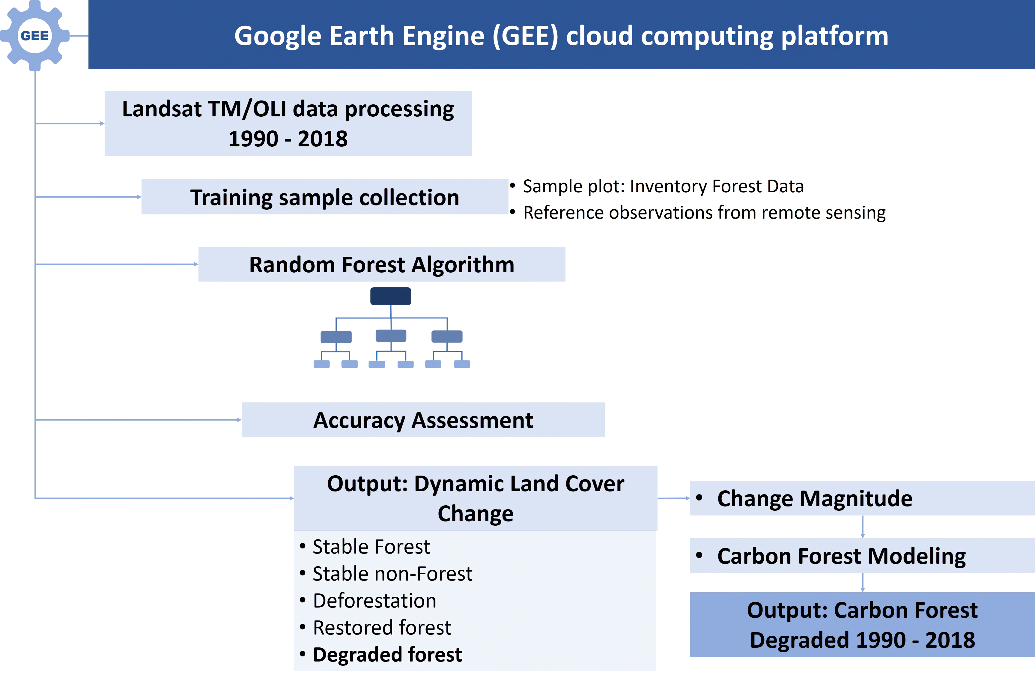
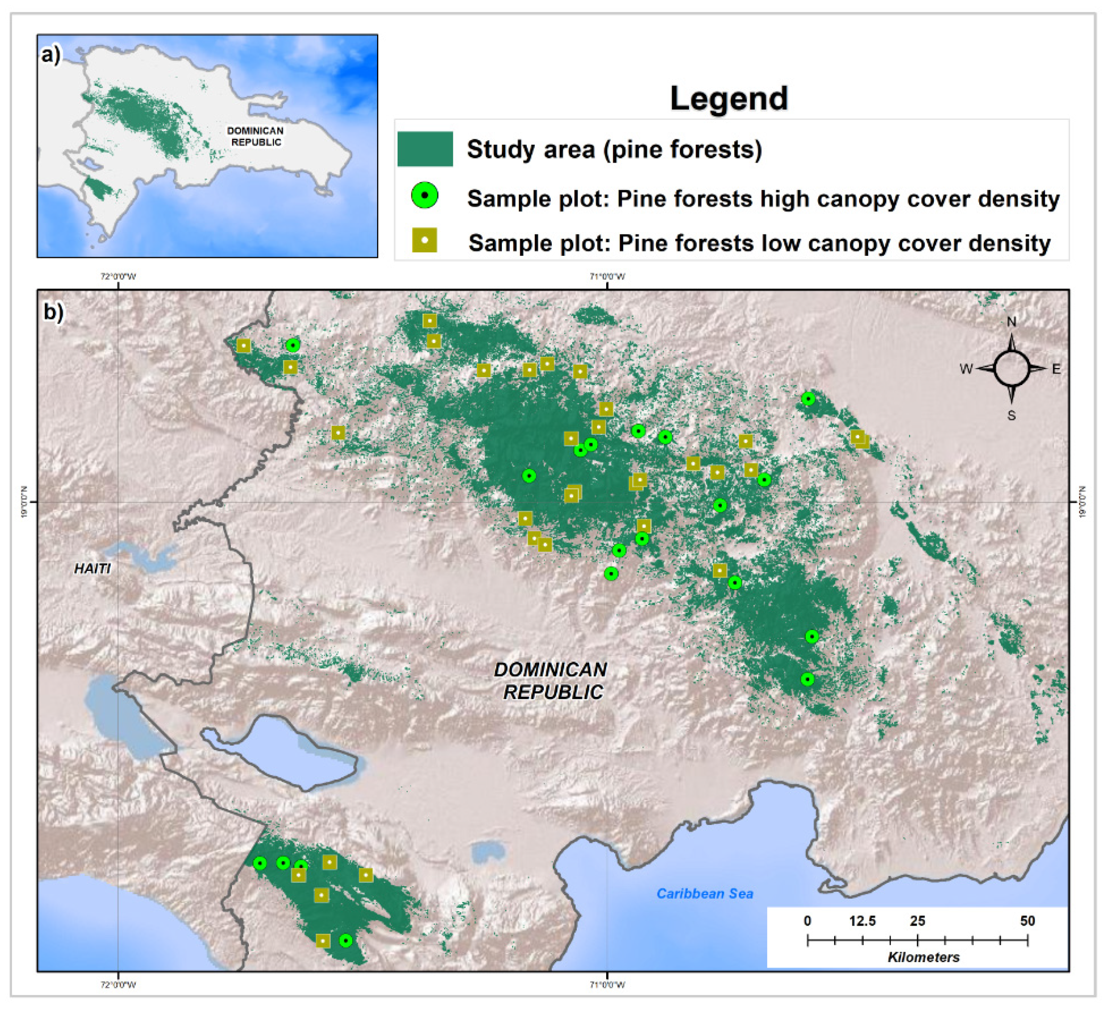
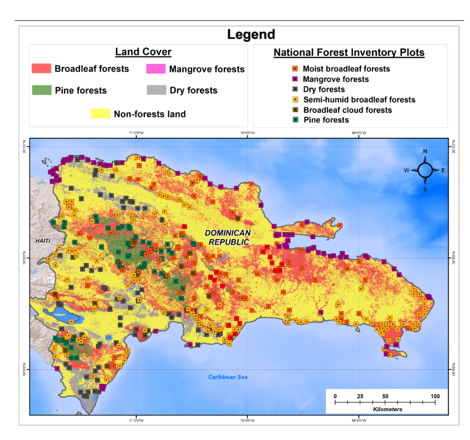
2.1. Study Area
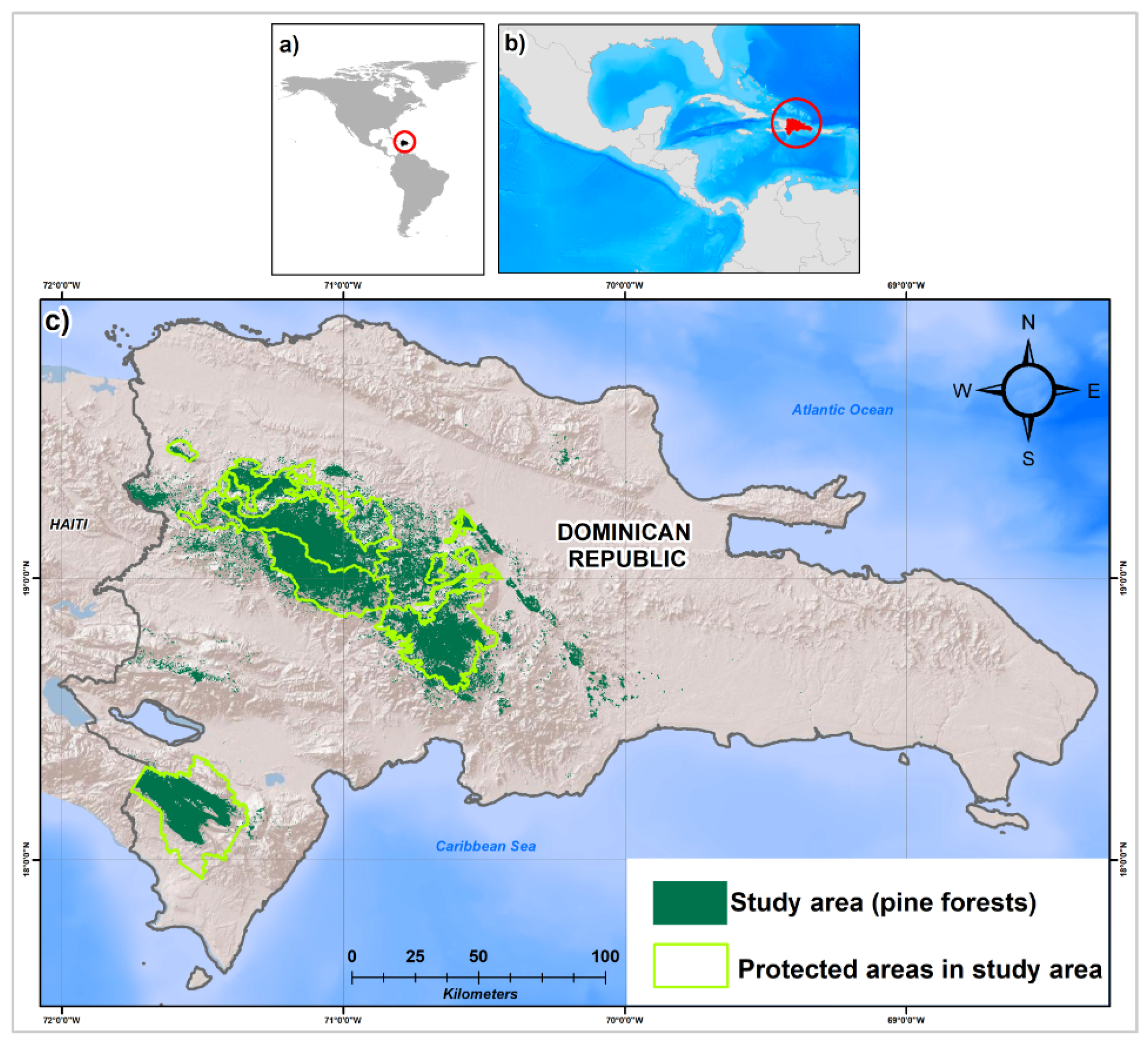
2.2. Forest, Deforestation, and Degradation Definitions
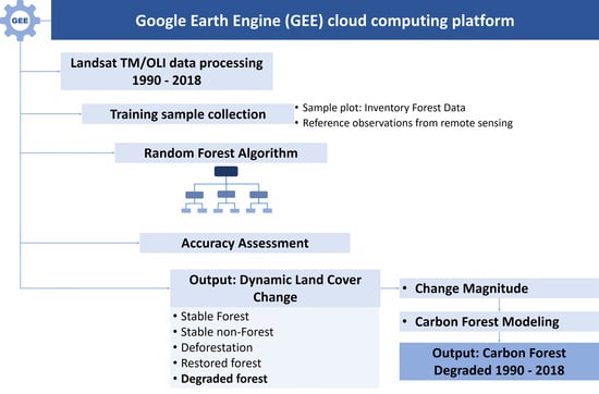
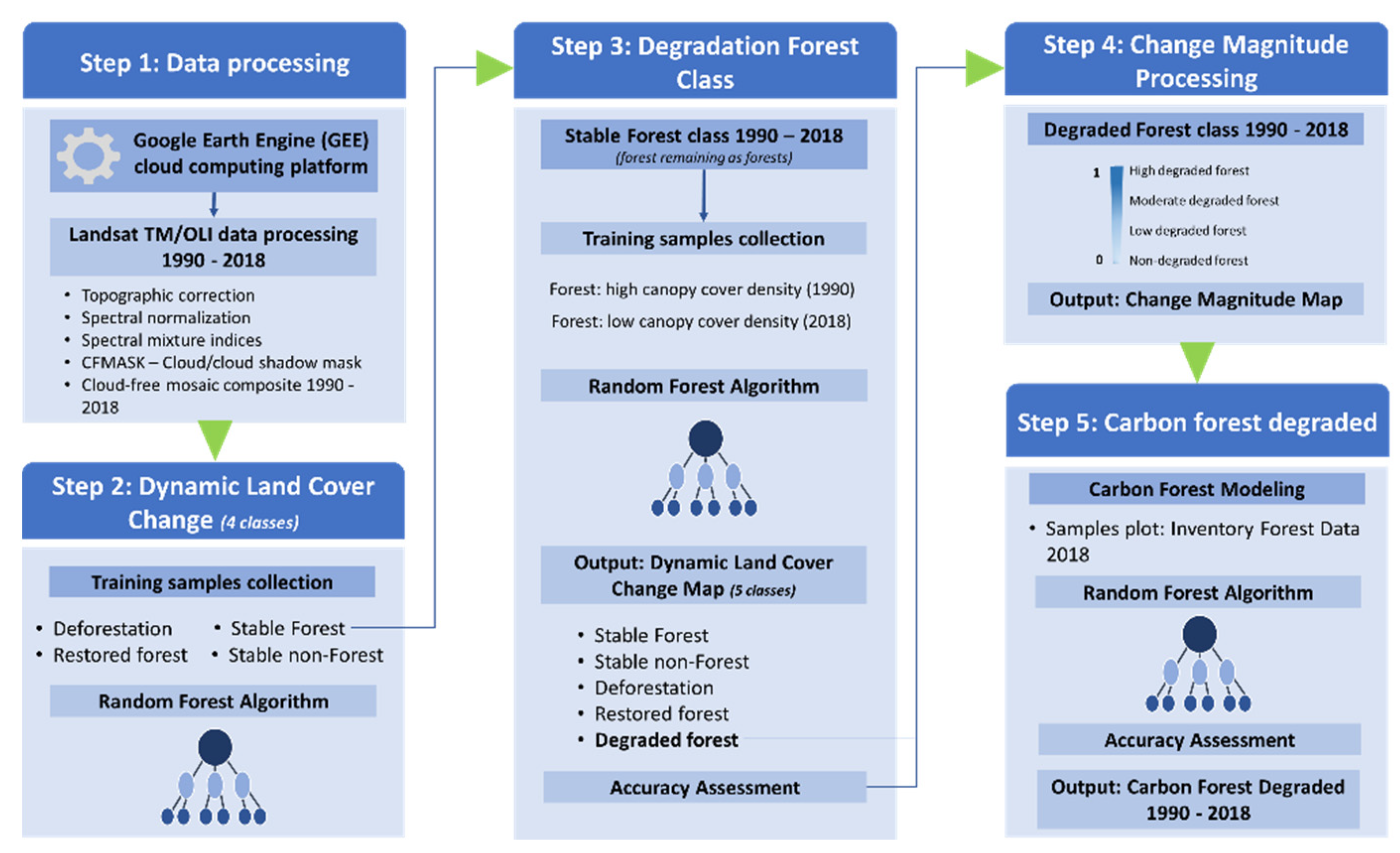
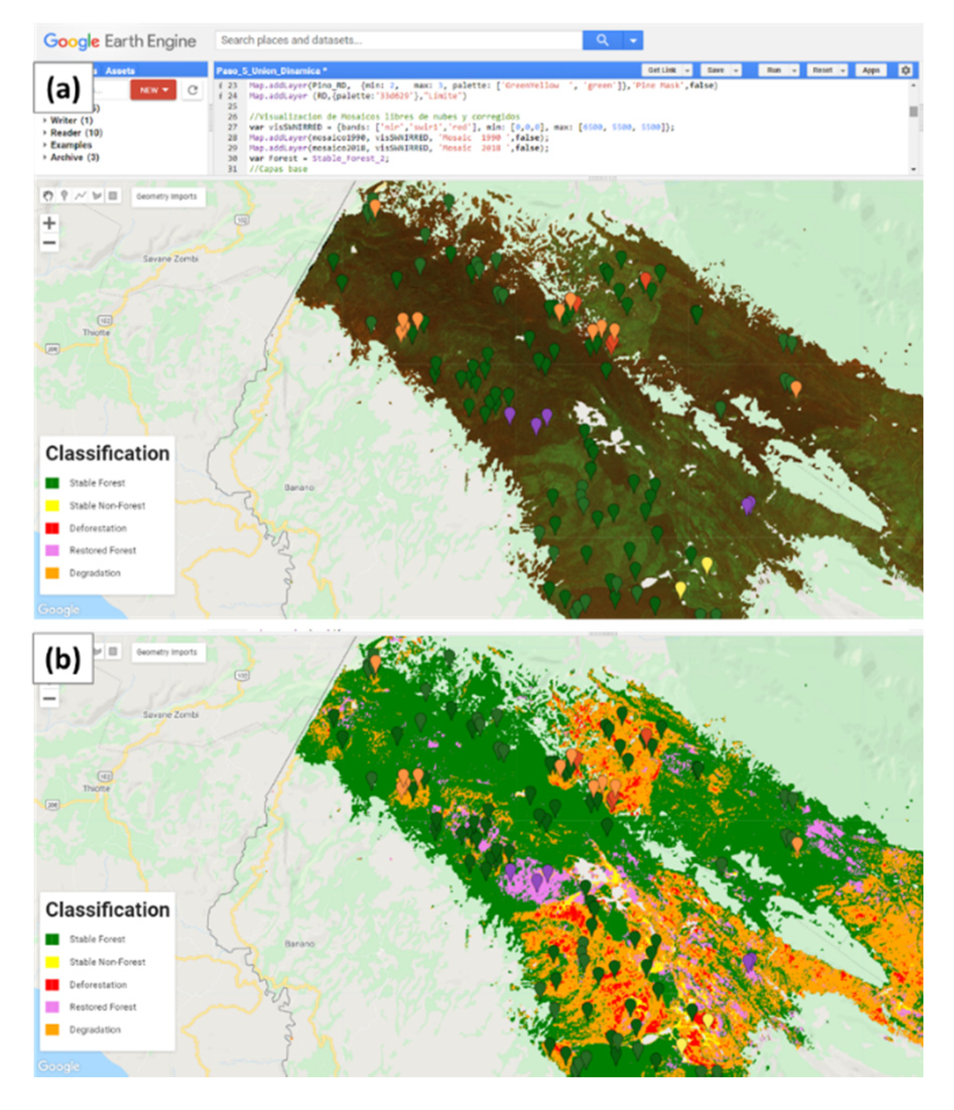
2.3. Method
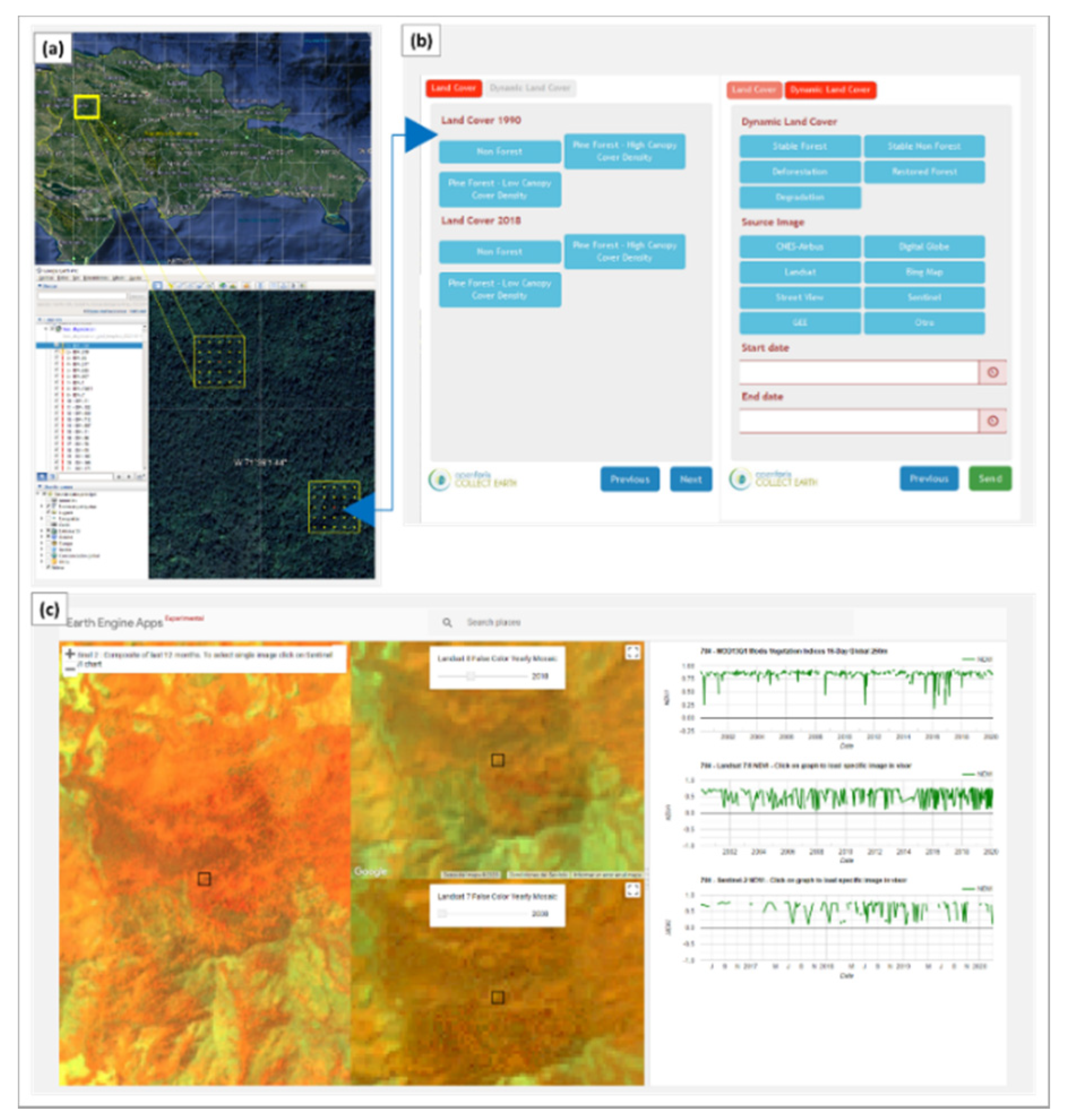
2.4. Reference Data
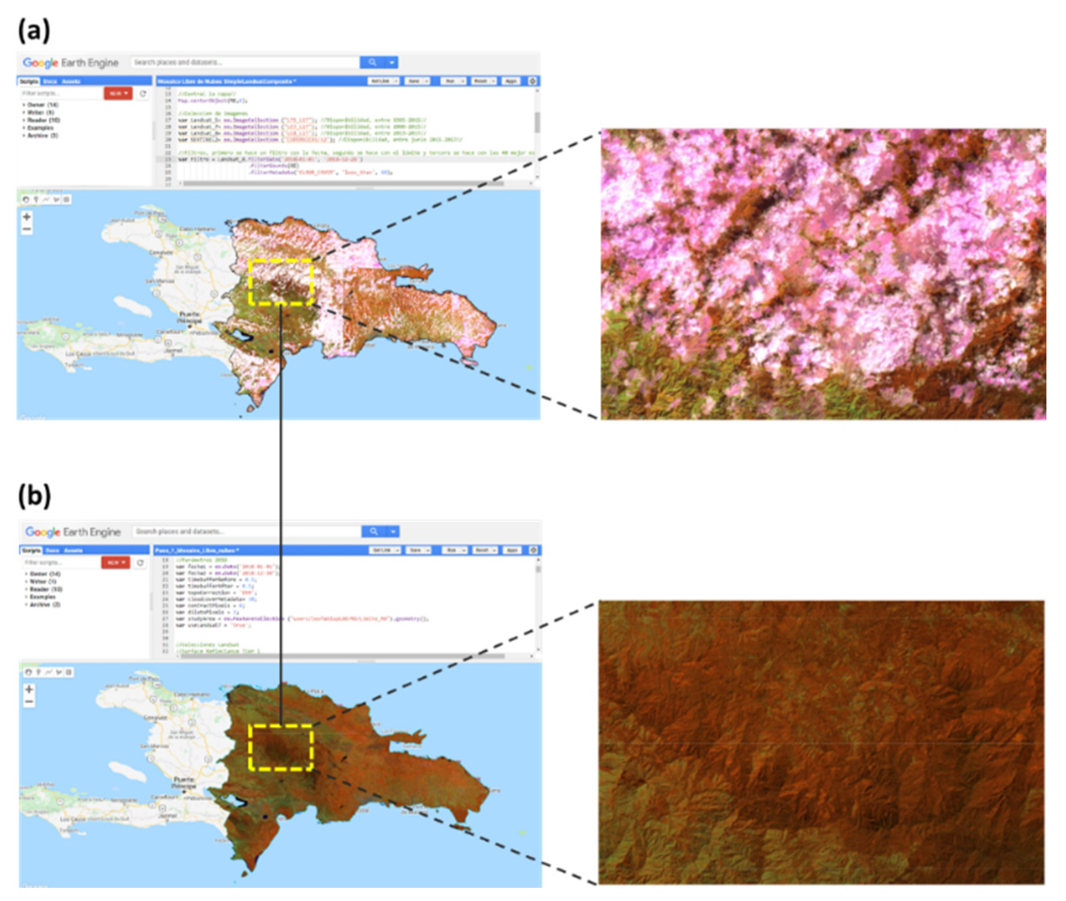
2.4.1. Landsat TM/OLI Data Processing
2.4.2. Field Inventory Data
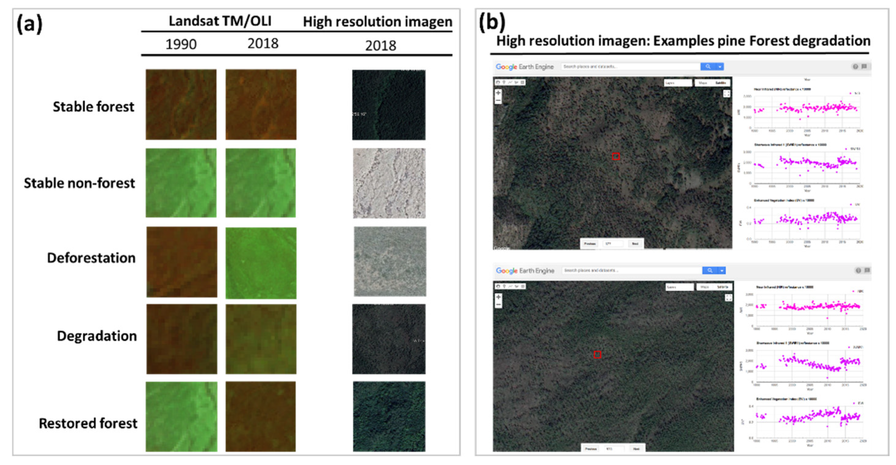
2.5. Classification of Dynamic Land Cover Change
Land Cover Change Samples
2.6. Carbon Stock and Change Magnitude
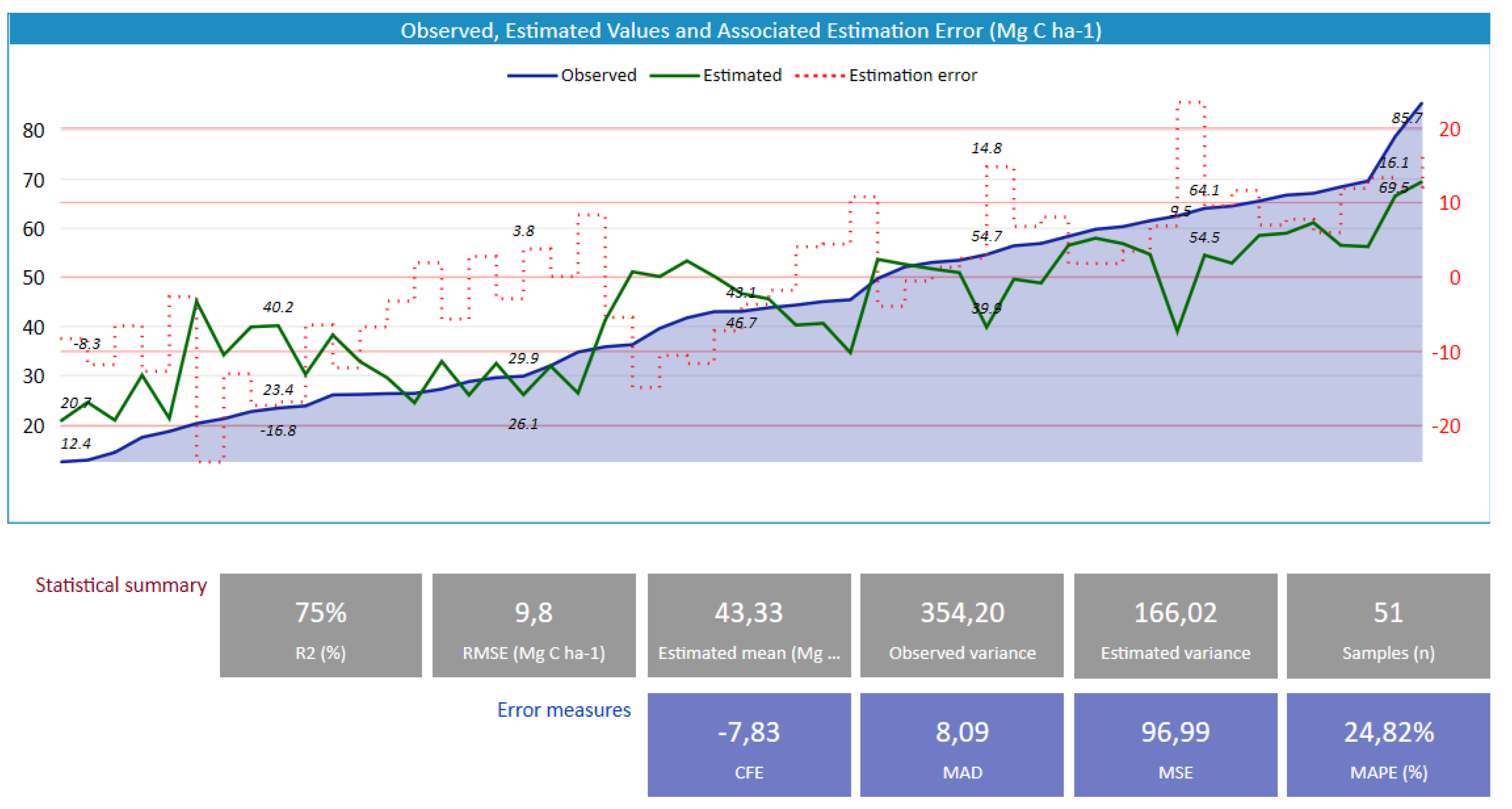
2.7. Model Evaluation: Carbon Stock
2.8. Accuracy Assessment and Analysis
3. Results
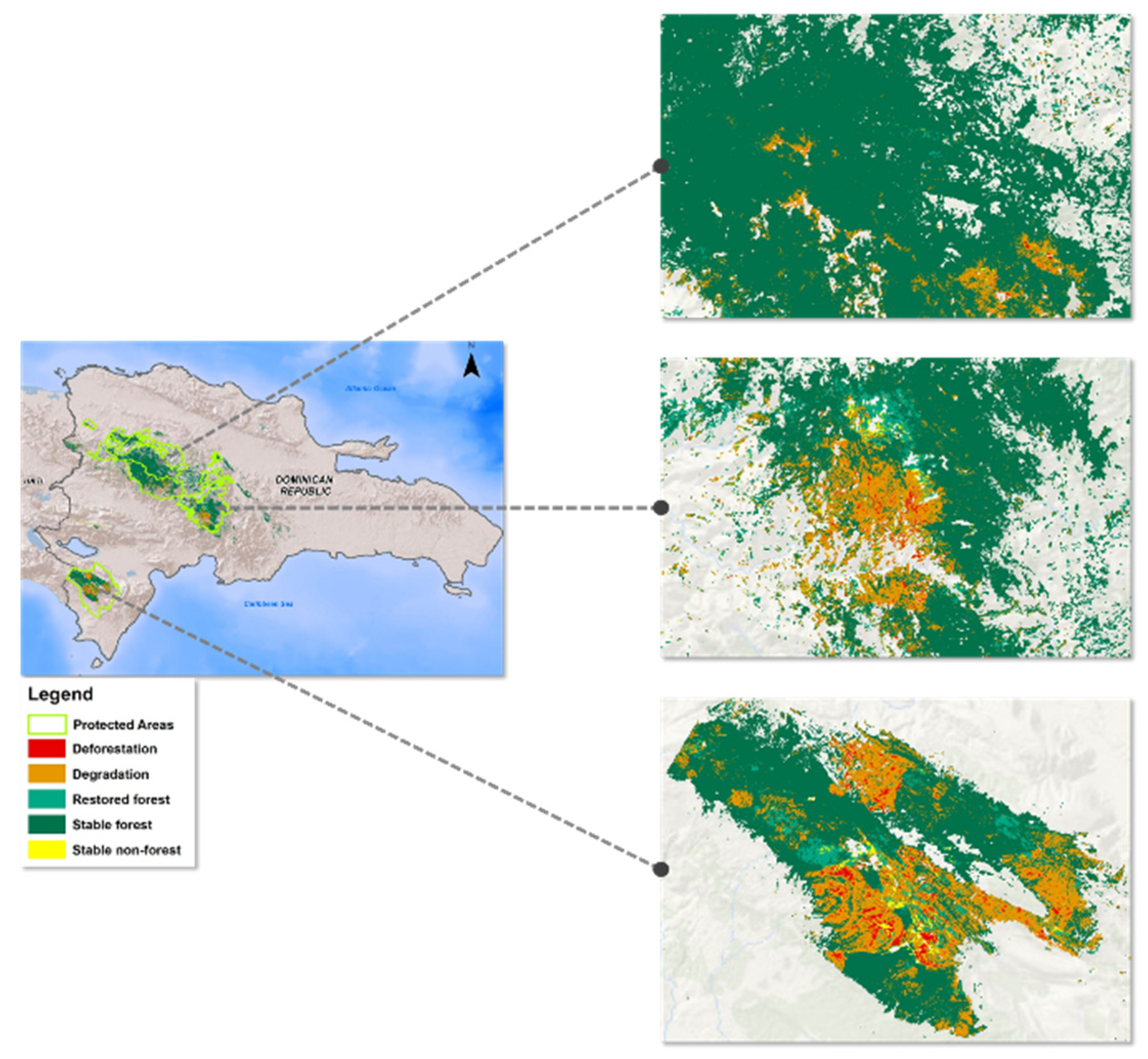
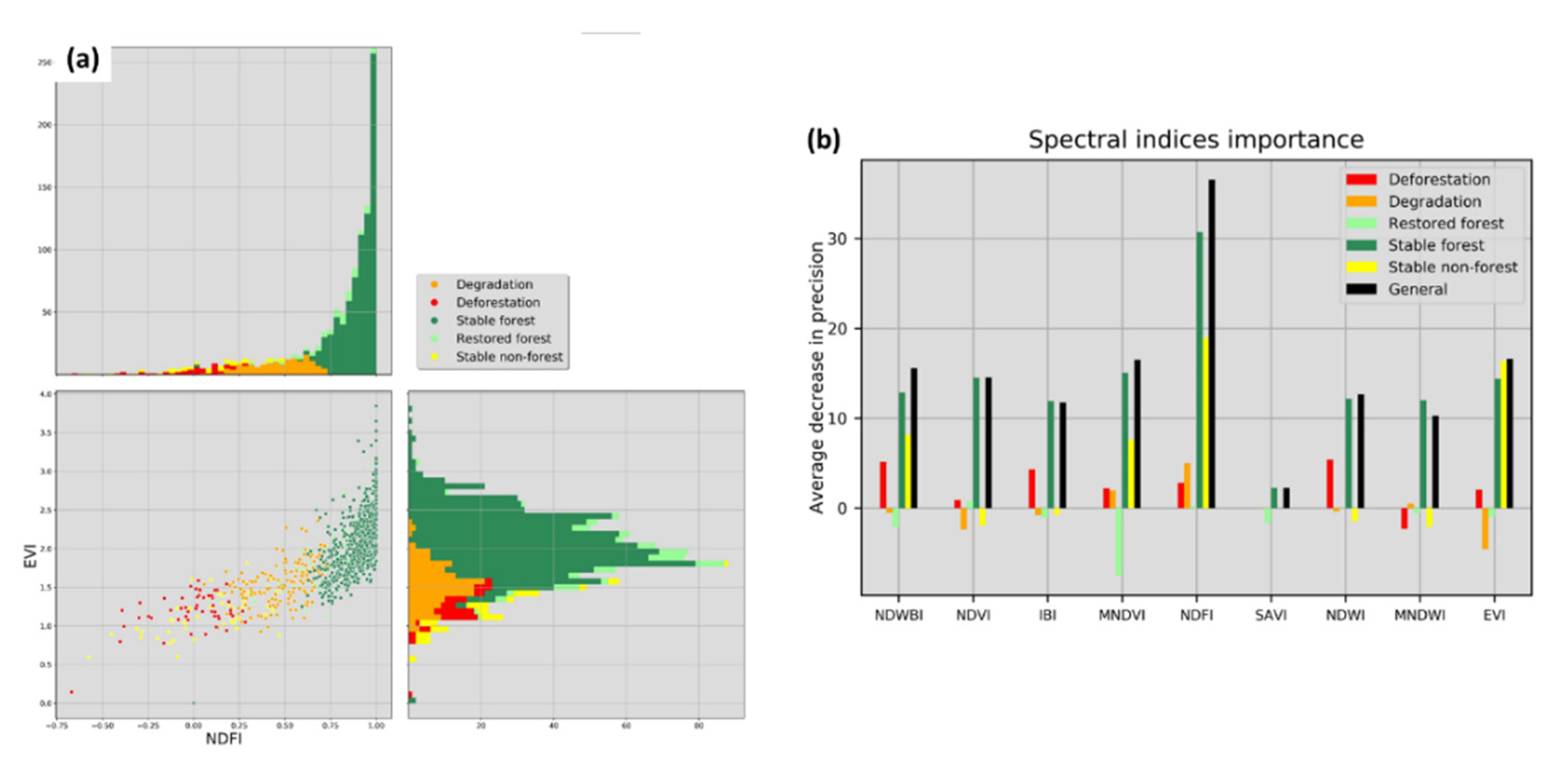
3.1. Dynamic Land Cover Changes from 1990 to 2018
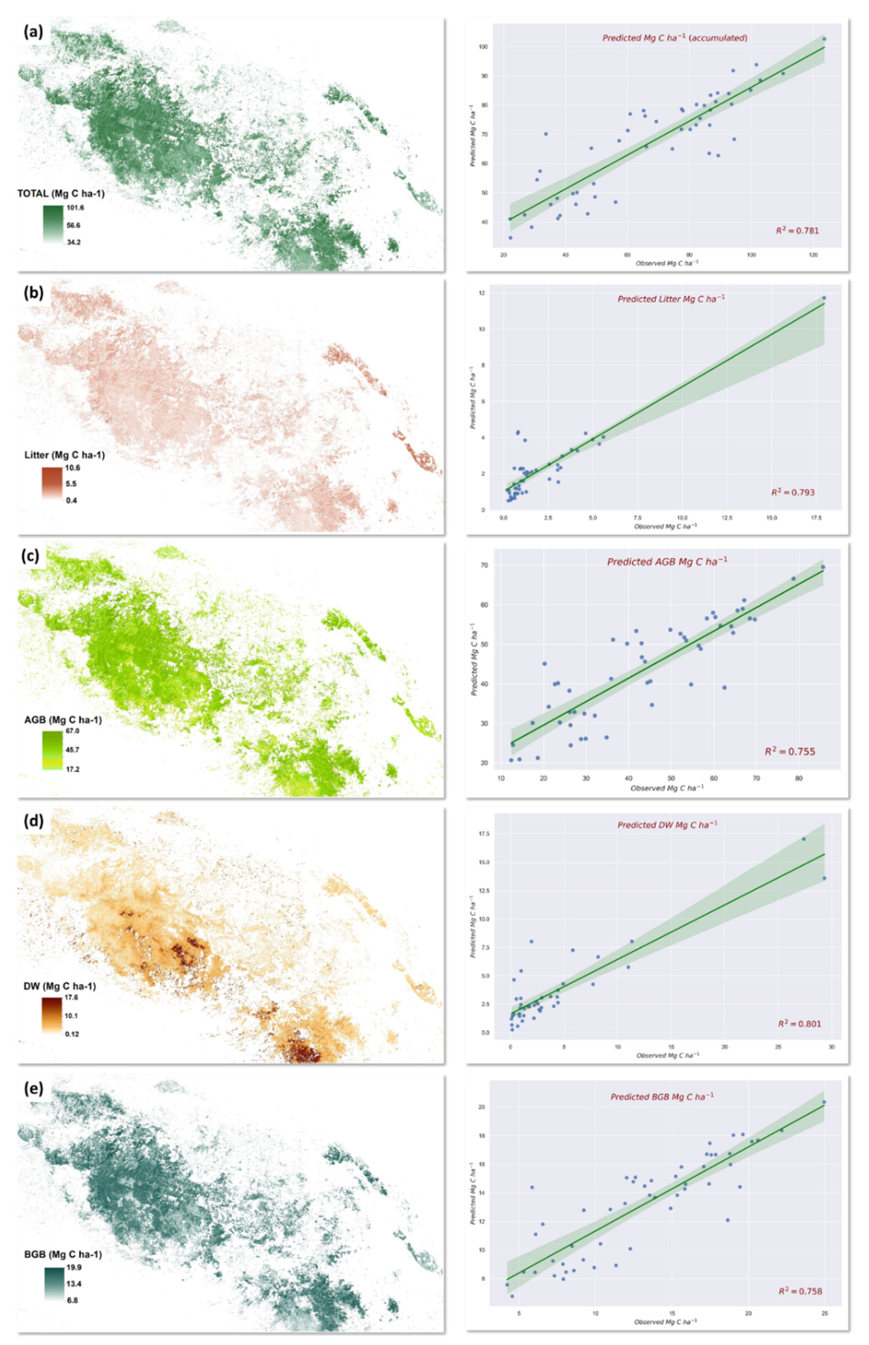
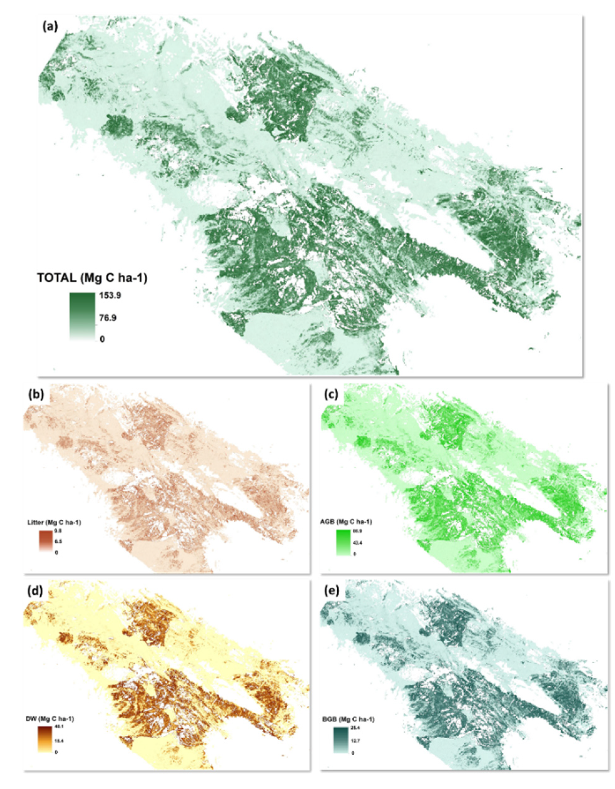
3.2. Carbon Stock
3.3. Carbon Degraded in the 1990–2018 Period
4. Discussion
4.1. Validation of Dynamic Land Cover Change Map from the 1990–2018 Period
4.2. Carbon Model Assessment
4.3. Google Earth Engine Platform
5. Conclusions
Author Contributions
Funding
Acknowledgments
Conflicts of Interest
Appendix A
Appendix B
Appendix C

| Spectral Indices | Equation |
|---|---|
| Normalized Difference Vegetation Index (NDVI) [73] | |
| Normalized Difference Spectral Vector (NDSV) [74] | where and are two generic bands. |
| Enhanced Vegetation Index (EVI) [50] | |
| Soil Adjust Vegetation Index (SAVI) [51] | |
| Index-Based Built-Up Index (IBI) [52] | |
| Near-Infrared Reflectance of Vegetation (NIRv) [75] | |
| Normalized Difference Fraction Index (NDFI) [52] | where: |
Appendix D
| ID | Class | AGB (Mg C ha−1) | BGB (Mg C ha−1) | Litter (Mg C ha−1) | DW (Mg C ha−1) | Total Accumulated (Mg C ha−1) | Long | Lat |
|---|---|---|---|---|---|---|---|---|
| 1 | Pine forest: low canopy cover density | 18.6 | 7.9 | 0.4 | 0.0 | 37.5 | −71.363 | 19.371 |
| 2 | Pine forest: high canopy cover density | 26.2 | 7.2 | 1.3 | 0.0 | 35.2 | −71.642 | 19.321 |
| 3 | Pine forest: low canopy cover density | 12.4 | 4.6 | 0.5 | 0.3 | 22.2 | −71.743 | 19.321 |
| 4 | Pine forest: low canopy cover density | 17.4 | 5.3 | 0.6 | 1.2 | 26.8 | −71.354 | 19.330 |
| 5 | Pine forest: low canopy cover density | 34.8 | 11.3 | 0.6 | 2.2 | 56.1 | −71.647 | 19.277 |
| 6 | Pine forest: low canopy cover density | 85.7 | 25.0 | 3.3 | 2.9 | 123.6 | −71.158 | 19.272 |
| 7 | Pine forest: low canopy cover density | 56.4 | 15.3 | 2.6 | 2.7 | 77.4 | −71.055 | 19.268 |
| 8 | Pine forest: low canopy cover density | 49.8 | 15.6 | 1.8 | 2.2 | 77.5 | −71.122 | 19.284 |
| 9 | Pine forest: low canopy cover density | 41.8 | 12.0 | 0.9 | 7.7 | 65.2 | −71.252 | 19.270 |
| 10 | Pine forest: high canopy cover density | 43.0 | 13.2 | 4.6 | 2.5 | 69.3 | −70.589 | 19.212 |
| 11 | Pine forest: low canopy cover density | 29.6 | 10.3 | 0.4 | 0.1 | 49.1 | −71.001 | 19.191 |
| 12 | Pine forest: high canopy cover density | 58.4 | 17.5 | 4.1 | 0.5 | 86.8 | −71.054 | 19.107 |
| 13 | Pine forest: high canopy cover density | 27.3 | 8.5 | 3.1 | 0.8 | 43.7 | −70.936 | 19.146 |
| 14 | Pine forest: high canopy cover density | 64.1 | 20.2 | 3.8 | 0.8 | 99.8 | −70.881 | 19.134 |
| 15 | Pine forest: high canopy cover density | 68.4 | 20.6 | 1.4 | 4.4 | 102.8 | −71.033 | 19.119 |
| 16 | Pine forest: low canopy cover density | 60.3 | 17.9 | 5.0 | 3.7 | 92.7 | −70.478 | 19.124 |
| 17 | Pine forest: low canopy cover density | 59.8 | 17.3 | 1.2 | 2.4 | 84.8 | −70.488 | 19.134 |
| 18 | Pine forest: low canopy cover density | 23.4 | 9.2 | 0.9 | 4.0 | 48.3 | −71.073 | 19.131 |
| 19 | Pine forest: low canopy cover density | 45.4 | 12.3 | 1.3 | 27.4 | 86.4 | −70.717 | 19.125 |
| 20 | Pine forest: low canopy cover density | 29.9 | 8.1 | 0.3 | 0.0 | 38.2 | −71.550 | 19.143 |
| 21 | Pine forest: low canopy cover density | 52.1 | 15.9 | 1.1 | 4.4 | 80.2 | −71.017 | 19.154 |
| 22 | Pine forest: high canopy cover density | 53.5 | 15.2 | 1.3 | 4.9 | 77.9 | −71.159 | 19.055 |
| 23 | Pine forest: high canopy cover density | 45.1 | 14.9 | 1.6 | 2.8 | 74.5 | −70.679 | 19.046 |
| 24 | Pine forest: low canopy cover density | 39.6 | 12.6 | 0.8 | 0.0 | 60.1 | −71.067 | 19.022 |
| 25 | Pine forest: low canopy cover density | 32.0 | 9.2 | 5.6 | 0.7 | 49.5 | −70.706 | 19.066 |
| 26 | Pine forest: low canopy cover density | 78.7 | 22.2 | 3.0 | 2.9 | 110.2 | −70.824 | 19.079 |
| 27 | Pine forest: low canopy cover density | 26.3 | 7.3 | 3.2 | 5.8 | 43.4 | −70.941 | 19.039 |
| 28 | Pine forest: low canopy cover density | 35.9 | 11.0 | 2.6 | 29.3 | 83.4 | −70.933 | 19.046 |
| 29 | Pine forest: low canopy cover density | 20.3 | 5.9 | 5.4 | 0.8 | 33.7 | −70.775 | 19.061 |
| 30 | Pine forest: high canopy cover density | 43.8 | 13.7 | 17.9 | 0.1 | 82.3 | −70.769 | 18.994 |
| 31 | Pine forest: low canopy cover density | 43.1 | 11.9 | 0.9 | 0.3 | 57.3 | −71.073 | 19.013 |
| 32 | Pine forest: low canopy cover density | 61.5 | 17.1 | 0.6 | 8.2 | 89.1 | −71.167 | 18.967 |
| 33 | Pine forest: low canopy cover density | 21.2 | 6.1 | 0.6 | 1.6 | 30.8 | −70.925 | 18.952 |
| 34 | Pine forest: high canopy cover density | 69.6 | 18.8 | 0.7 | 4.4 | 93.6 | −70.975 | 18.902 |
| 35 | Pine forest: high canopy cover density | 56.9 | 15.8 | 0.7 | 11.3 | 86.5 | −70.929 | 18.926 |
| 36 | Pine forest: low canopy cover density | 28.8 | 9.9 | 0.4 | 0.1 | 47.2 | −71.148 | 18.927 |
| 37 | Pine forest: low canopy cover density | 64.5 | 17.4 | 0.2 | 0.0 | 82.1 | −71.126 | 18.913 |
| 38 | Pine forest: high canopy cover density | 62.5 | 18.6 | 0.7 | 0.9 | 89.3 | −70.738 | 18.836 |
| 39 | Pine forest: high canopy cover density | 66.8 | 18.8 | 0.0 | 0.2 | 88.5 | −70.992 | 18.855 |
| 40 | Pine forest: low canopy cover density | 23.8 | 7.9 | 0.3 | 0.0 | 37.3 | −70.770 | 18.861 |
| 41 | Pine forest: high canopy cover density | 22.7 | 6.5 | 1.0 | 0.0 | 31.8 | −70.581 | 18.726 |
| 42 | Pine forest: high canopy cover density | 36.3 | 12.5 | 1.0 | 1.3 | 60.9 | −70.590 | 18.639 |
| 43 | Pine forest: high canopy cover density | 67.1 | 19.0 | 1.2 | 11.0 | 101.6 | −71.709 | 18.263 |
| 44 | Pine forest: high canopy cover density | 53.1 | 17.6 | 3.0 | 1.1 | 86.7 | −71.662 | 18.263 |
| 45 | Pine forest: low canopy cover density | 26.4 | 8.6 | 1.0 | 1.0 | 42.4 | −71.568 | 18.265 |
| 46 | Pine forest: high canopy cover density | 65.5 | 19.6 | 0.8 | 1.0 | 94.1 | −71.625 | 18.256 |
| 47 | Pine forest: low canopy cover density | 14.4 | 6.0 | 0.6 | 0.0 | 29.1 | −71.493 | 18.238 |
| 48 | Pine forest: low canopy cover density | 12.8 | 4.2 | 0.3 | 2.0 | 22.1 | −71.584 | 18.197 |
| 49 | Pine forest: low canopy cover density | 26.1 | 13.5 | 1.1 | 0.9 | 65.7 | −71.631 | 18.239 |
| 50 | Pine forest: high canopy cover density | 54.7 | 19.4 | 1.3 | 1.7 | 94.5 | −71.534 | 18.105 |
| 51 | Pine forest: low canopy cover density | 44.4 | 13.9 | 0.8 | 0.0 | 66.1 | −71.581 | 18.104 |
Appendix E

References
- Friedl, M.A.; McIver, D.K.; Hodges, J.C.F.; Zhang, X.Y.; Muchoney, D.; Strahler, A.H.; Woodcock, C.E.; Gopal, S.; Schneider, A.; Cooper, A.; et al. Global land cover mapping from MODIS: Algorithms and early results. Remote Sens. Environ. 2002, 83, 287–302. [Google Scholar] [CrossRef]
- Wulder, M.A.; White, J.C.; Goward, S.N.; Masek, J.G.; Irons, J.R.; Herold, M.; Cohen, W.B.; Loveland, T.R.; Woodcock, C.E. Landsat continuity: Issues and opportunities for land cover monitoring. Remote Sens. Environ. 2008, 112, 955–969. [Google Scholar] [CrossRef]
- Pearson, T.R.H.; Brown, S.; Murray, L.; Sidman, G. Greenhouse gas emissions from tropical forest degradation: An underestimated source. Carbon Balance Manag. 2017, 12, 3. [Google Scholar] [CrossRef] [PubMed]
- Harris, N.L.; Brown, S.; Hagen, S.C.; Saatchi, S.S.; Petrova, S.; Salas, W.; Hansen, M.C.; Potapov, P.V.; Lotsch, A. Baseline Map of Carbon Emissions from Deforestation in Tropical Regions. Science 2012, 336, 1573. [Google Scholar] [CrossRef]
- Chazdon, R.L.; Brancalion, P.H.S.; Laestadius, L.; Bennett-Curry, A.; Buckingham, K.; Kumar, C.; Moll-Rocek, J.; Vieira, I.C.G.; Wilson, S.J. When is a forest a forest? Forest concepts and definitions in the era of forest and landscape restoration. Ambio 2016, 45, 538–550. [Google Scholar] [CrossRef]
- Arana Pardo, J.I.; Birdsey, R.; Boehm, M.; Daka, J.; Kobayashi, S.; Lund, H.G.; Michalak, R.; Takahashi, M. IPCC Report on Definitions and Methodological Options to Inventory Emissions from Direct Human-induced Degradation of Forests and Devegetation of Other Vegetation Types; Eggleston, H.S., Buendia, L., Miwa, K., Ngara, T., Tanabe, K., Eds.; Institute for Global Environmental Strategies (IGES): Kanagawa, Japan, 2003. [Google Scholar]
- van der Werf, G.R.; Morton, D.C.; DeFries, R.S.; Olivier, J.G.J.; Kasibhatla, P.S.; Jackson, R.B.; Collatz, G.J.; Randerson, J.T. CO2 emissions from forest loss. Nat. Geosci. 2009, 2, 737. [Google Scholar] [CrossRef]
- Metz, B.; Davidson, R.; Bosch, R.; Dave, R.; Meyer, L. Climate Change 2007: Mitigation of Climate Change; Cambridge University Press: Cambridge, UK, 2007. [Google Scholar]
- UNFCCC. Addendum Part Two: Action Taken by the Conference of the Parties at Its Sixteenth Session. In Proceedings of the Report of the Conference of the Parties on Its Sixteenth Session, Cancún, Mexico, 29 November–10 December 2011. [Google Scholar]
- Ochieng, R.M.; Visseren-Hamakers, I.J.; Arts, B.; Brockhaus, M.; Herold, M. Institutional effectiveness of REDD+ MRV: Countries progress in implementing technical guidelines and good governance requirements. Environ. Sci. Policy 2016, 61, 42–52. [Google Scholar] [CrossRef]
- Goetz, S.J.; Hansen, M.; Houghton, R.A.; Walker, W.; Laporte, N.; Busch, J. Measurement and monitoring needs, capabilities and potential for addressing reduced emissions from deforestation and forest degradation under REDD+. Environ. Res. Lett. 2015, 10, 123001. [Google Scholar] [CrossRef]
- Milne, R.; Jallow, P. Basis for Consistent Representation of Land Areas. In IPCC Good Practice Guidance for LULUCF; Institute for Global Environmental Strategies (IGES): Kanagawa, Japan, 2003. [Google Scholar]
- Woodcock, C. Free Access to Landsat Imagery Teach by the Book Science Education. Science 2008, 80, 1011–1012. [Google Scholar] [CrossRef]
- Hansen, M.C.; Potapov, P.V.; Moore, R.; Hancher, M.; Turubanova, S.A.; Tyukavina, A.; Thau, D.; Stehman, S.V.; Goetz, S.J.; Loveland, T.R.; et al. High-Resolution Global Maps of 21st-Century Forest Cover Change. Science 2013, 342, 850. [Google Scholar] [CrossRef]
- Herold, M.; Hirata, Y.; Laake, P.V.; Asner, G.; Heymell, V.; Román-cuesta, R.M. A review of methods to measure and monitor historical forest degradation. Unasylva 2011, 62, 16–24. [Google Scholar]
- Hosonuma, N.; Herold, M.; De Sy, V.; De Fries, R.S.; Brockhaus, M.; Verchot, L.; Angelsen, A.; Romijn, E. An assessment of deforestation and forest degradation drivers in developing countries. Environ. Res. Lett. 2012, 7, 044009. [Google Scholar] [CrossRef]
- Chambers, J.Q.; Asner, G.P.; Morton, D.C.; Anderson, L.O.; Saatchi, S.S.; Espírito-Santo, F.D.B.; Palace, M.; Souza, C., Jr. Regional ecosystem structure and function: Ecological insights from remote sensing of tropical forests. Trends Ecol. Evol. 2007, 22, 414–423. [Google Scholar] [CrossRef]
- De Sy, V.; Herold, M.; Achard, F.; Asner, G.P.; Held, A.; Kellndorfer, J.; Verbesselt, J. Synergies of multiple remote sensing data sources for REDD+ monitoring. Curr. Opin. Environ. Sustain. 2012, 4, 696–706. [Google Scholar] [CrossRef]
- Woodcock, C.E.; Macomber, S.A.; Pax-Lenney, M.; Cohen, W.B. Monitoring large areas for forest change using Landsat: Generalization across space, time and Landsat sensors. Remote Sens. Environ. 2001, 78, 194–203. [Google Scholar] [CrossRef]
- Zhu, Z.; Woodcock, C.E. Continuous change detection and classification of land cover using all available Landsat data. Remote Sens. Environ. 2014, 144, 152–171. [Google Scholar] [CrossRef]
- Gorelick, N.; Hancher, M.; Dixon, M.; Ilyushchenko, S.; Thau, D.; Moore, R. Google Earth Engine: Planetary-scale geospatial analysis for everyone. Remote Sens. Environ. 2017, 202, 18–27. [Google Scholar] [CrossRef]
- Azzari, G.; Lobell, D.B. Landsat-based classification in the cloud: An opportunity for a paradigm shift in land cover monitoring. Remote Sens. Environ. 2017, 202, 64–74. [Google Scholar] [CrossRef]
- Chen, B.; Xiao, X.; Li, X.; Pan, L.; Doughty, R.; Ma, J.; Dong, J.; Qin, Y.; Zhao, B.; Wu, Z.; et al. A mangrove forest map of China in 2015: Analysis of time series Landsat 7/8 and Sentinel-1A imagery in Google Earth Engine cloud computing platform. Isprs, J. Photogramm. Remote Sens. 2017, 131, 104–120. [Google Scholar] [CrossRef]
- Dong, J.; Xiao, X.; Menarguez, M.A.; Zhang, G.; Qin, Y.; Thau, D.; Biradar, C.; Moore, B. Mapping paddy rice planting area in northeastern Asia with Landsat 8 images, phenology-based algorithm and Google Earth Engine. Remote Sens. Environ. 2016, 185, 142–154. [Google Scholar] [CrossRef]
- Goldblatt, R.; Stuhlmacher, M.F.; Tellman, B.; Clinton, N.; Hanson, G.; Georgescu, M.; Wang, C.; Serrano-Candela, F.; Khandelwal, A.K.; Cheng, W.-H.; et al. Using Landsat and nighttime lights for supervised pixel-based image classification of urban land cover. Remote Sens. Environ. 2018, 205, 253–275. [Google Scholar] [CrossRef]
- Huang, H.; Chen, Y.; Clinton, N.; Wang, J.; Wang, X.; Liu, C.; Gong, P.; Yang, J.; Bai, Y.; Zheng, Y.; et al. Mapping major land cover dynamics in Beijing using all Landsat images in Google Earth Engine. Remote Sens. Environ. 2017, 202, 166–176. [Google Scholar] [CrossRef]
- Orvis, K.H. The highest mountain in the Caribbean: Controversy and resolution via GPS. Caribb. J. Sci. 2003, 39, 378–380. [Google Scholar]
- SEMARENA. Perfil Nacional Para Evaluar Las Capacidades Nacionales de Implementación del Principio 10 de la Declaración de Rio; Secretary of State for the Environment and Natural Resources: Santo Domingo, Dominican Republic, 2008; p. 119. [Google Scholar]
- Kennedy, L.M.; Horn, S.P.; Orvis, K.H. Modern pollen spectra from the highlands of the Cordillera Central, Dominican Republic. Rev. Palaeobot. Palynol. 2005, 137, 51–68. [Google Scholar] [CrossRef]
- Darrow, W.K.; Zanoni, T. Hispaniolan pine (Pinus occidentalis Swartz) a little known sub-tropical pine of economic potential. Commonw. For. Rev. 1990, 69, 133–146. [Google Scholar]
- MARN. Analysis of the Direct and Indirect Drivers of Deforestation and Forest Degradation (DD) in the Dominican Republic; Ministry of Environment and Natural Resources: Santo Domingo, Dominican Republic, 2018; p. 161. [Google Scholar]
- FAO. Global Forest Resources Assessment 2015; UN Food and Agriculture Organization: Rome, Italy, 2015. [Google Scholar]
- Feliz, K.; Rodríguez, L.; Galán, M.; Ovidio, R.; Vargas, O.; de Jong, B. Dominican Republic Reference Emissions Levels/Forest Reference Levels; Ministry of Environment and Natural Resources: Santo Domingo, Dominican Republic, 2019; p. 78. Available online: https://redd.unfccc.int/files/nrfe_-_nrf_rep._dom_revgov2.pdf (accessed on 18 March 2020).
- Romero-Sanchez, M.E.; Ponce-Hernandez, R. Assessing and Monitoring Forest Degradation in a Deciduous Tropical Forest in Mexico via Remote Sensing Indicators. Forests 2017, 8, 302. [Google Scholar] [CrossRef]
- Thompson, I.D.; Guariguata, M.R.; Okabe, K.; Bahamondez, C.; Nasi, R.; Heymell, V.; Sabogal, C. An Operational Framework for Defining and Monitoring Forest Degradation. Ecol. Soc. 2013, 18, 20. [Google Scholar] [CrossRef]
- Masek, J.G.; Vermote, E.F.; Saleous, N.; Wolfe, R.; Hall, F.G.; Huemmrich, K.F.; Gao, F.; Kutler, J.; Lim, T.K. LEDAPS Calibration, Reflectance, Atmospheric Correction Preprocessing Code, Version 2; ORNL Distributed Active Archive Center: Oak Ridge, TN, USA, 2013. [Google Scholar]
- Vermote, E.; Justice, C.; Claverie, M.; Franch, B. Preliminary analysis of the performance of the Landsat 8/OLI land surface reflectance product. Remote Sens. Environ. 2016, 185, 46–56. [Google Scholar] [CrossRef]
- Zhu, Z.; Woodcock, C.E. Object-based cloud and cloud shadow detection in Landsat imagery. Remote Sens. Environ. 2012, 118, 83–94. [Google Scholar] [CrossRef]
- Foga, S.; Scaramuzza, P.L.; Guo, S.; Zhu, Z.; Dilley, R.D.; Beckmann, T.; Schmidt, G.L.; Dwyer, J.L.; Joseph Hughes, M.; Laue, B. Cloud detection algorithm comparison and validation for operational Landsat data products. Remote Sens. Environ. 2017, 194, 379–390. [Google Scholar] [CrossRef]
- Goldblatt, R.; Rivera Ballesteros, A.; Burney, J. High Spatial Resolution Visual Band Imagery Outperforms Medium Resolution Spectral Imagery for Ecosystem Assessment in the Semi-Arid Brazilian Sertão. Remote Sens. 2017, 9, 1336. [Google Scholar] [CrossRef]
- Farr, T.G.; Rosen, P.A.; Caro, E.; Crippen, R.; Duren, R.; Hensley, S.; Kobrick, M.; Paller, M.; Rodriguez, E.; Roth, L.; et al. The Shuttle Radar Topography Mission. Rev. Geophys. 2007, 45. [Google Scholar] [CrossRef]
- Tan, B.; Masek, J.G.; Wolfe, R.; Gao, F.; Huang, C.; Vermote, E.F.; Sexton, J.O.; Ederer, G. Improved forest change detection with terrain illumination corrected Landsat images. Remote Sens. Environ. 2013, 136, 469–483. [Google Scholar] [CrossRef]
- Flood, N. Seasonal Composite Landsat TM/ETM+ Images Using the Medoid (a Multi-Dimensional Median). Remote Sens. 2013, 5, 6481. [Google Scholar] [CrossRef]
- GEE Developers. Compositing and Mosaicking in Google Earth Engine Cloud Platform. Google Developers. Available online: https://developers.google.com/earth-engine/ic_composite_mosaic (accessed on 16 December 2019).
- MARN. Emission Reductions Program. Document (ER-PD); Ministry of Environment and Natural Resources: Santo Domingo, Dominican Republic, 2019; p. 368. Available online: https://www.forestcarbonpartnership.org/country/dominican-republic (accessed on 15 February 2020).
- Milla, F.; Díaz, R.; Emanuelli, P. National Multipurpose Forest Inventory of the Dominican Republic 2014–2015. Planning and Protocol Elements for Measurement Operations. Available online: http://www.reddccadgiz.org/documentos/doc_1313366786.pdf.ElSalvador (accessed on 20 March 2020).
- Emanuelli, P.; Gonzales, J.; Nuñez, J.; Milla, F.; Duarte, E.; Mercedes, J.; Garrido, C.; Holmgren, A. National Forest Inventory of the Dominican Republic 2018. Final Report (ESP). Available online: http://www.reddccadgiz.org/documentos/doc_1984105887.pdf (accessed on 22 August 2019).
- Diaz, R.; Jiménez, A. National Forest Inventory of the Dominican Republic: Measure and Assess Forests in Order to Understand Their Diversity, Composition, Volume and biomass. Field Manual; REDD/CCAD-GIZ Regional Project and Ministry of Environment and Natural Resources: Santo Domingo, Dominican Republic, 2016; p. 48. [Google Scholar]
- Hansen, M.C.; Defries, R.S.; Townshend, J.R.G.; Sohlberg, R. Global land cover classification at 1 km spatial resolution using a classification tree approach. Int. J. Remote Sens. 2000, 21, 1331–1364. [Google Scholar] [CrossRef]
- Huete, A.R.; Liu, H.Q.; Batchily, K.; Van Leeuwen, W. A comparison of vegetation indices over a global set of TM images for EOS-MODIS. Remote Sens. Environ. 1997, 59, 440–451. [Google Scholar] [CrossRef]
- Huete, A.R. A soil-adjusted vegetation index (SAVI). Remote Sens. Environ. 1988, 25, 295–309. [Google Scholar] [CrossRef]
- Souza, C.M.; Roberts, D.A.; Cochrane, M.A. Combining spectral and spatial information to map canopy damage from selective logging and forest fires. Remote Sens. Environ. 2005, 98, 329–343. [Google Scholar] [CrossRef]
- Breiman, L. Random Forests. Mach. Learn. 2001, 45, 5–32. [Google Scholar] [CrossRef]
- Ma, W.; Domke, G.M.; Woodall, C.W.; D’Amato, A.W. Contemporary forest carbon dynamics in the northern U.S. associated with land cover changes. Ecol. Indic. 2020, 110, 105901. [Google Scholar] [CrossRef]
- Swingland, I.R.; Bettelheim, E.C.; Grace, J.; Prance, G.T.; Saunders, L.S.; Brown, S. Measuring, monitoring, and verification of carbon benefits for forest–based projects. Philos. Trans. R. Soc. Lond. Ser. A Math. Phys. Eng. Sci. 2002, 360, 1669–1683. [Google Scholar] [CrossRef]
- Díaz, R. Sánchez, R. Manual de Campo Inventario de Biomasa y Carbono en Sistemas No Bosque; Ministry of Environment and Natural Resources: Santo Domingo, Dominican Republic, 2017.
- MARN. Emission Reduction Program of the Dominican Republic: Contributions to Sustainable Livelihoods of Rural Communities and Carbon Enhancements; Ministry of Environment and Natural Resources: Santo Domingo, Dominican Republic, 2015; p. 68. Available online: https://www.forestcarbonpartnership.org/system/files/documents/Dominican%20Republic%20ER-PIN%20Final_0.pdf (accessed on 5 December 2019).
- Bullock, E.L.; Woodcock, C.E.; Olofsson, P. Monitoring tropical forest degradation using spectral unmixing and Landsat time series analysis. Remote Sens. Environ. 2020, 238, 110968. [Google Scholar] [CrossRef]
- Zhu, Z.; Woodcock, C.E.; Olofsson, P. Continuous monitoring of forest disturbance using all available Landsat imagery. Remote Sens. Environ. 2012, 122, 75–91. [Google Scholar] [CrossRef]
- Pasquarella, V.J.; Bradley, B.A.; Woodcock, C.E. Near-Real-Time Monitoring of Insect Defoliation Using Landsat Time Series. Forests 2017, 8, 275. [Google Scholar] [CrossRef]
- Tang, X.; Bullock, E.L.; Olofsson, P.; Estel, S.; Woodcock, C.E. Near real-time monitoring of tropical forest disturbance: New algorithms and assessment framework. Remote Sens. Environ. 2019, 224, 202–218. [Google Scholar] [CrossRef]
- Gómez, C.; White, J.C.; Wulder, M.A.; Alejandro, P. Historical forest biomass dynamics modelled with Landsat spectral trajectories. Isprs. J. Photogramm. Remote Sens. 2014, 93, 14–28. [Google Scholar] [CrossRef]
- Arlot, S.; Celisse, A. A survey of cross-validation procedures for model selection. Stat. Surv. 2010, 4, 40–79. [Google Scholar] [CrossRef]
- Olofsson, P.; Foody, G.M.; Herold, M.; Stehman, S.V.; Woodcock, C.E.; Wulder, M.A. Good practices for estimating area and assessing accuracy of land change. Remote Sens. Environ. 2014, 148, 42–57. [Google Scholar] [CrossRef]
- GFOI. Integration of Remote-Sensing and Ground-Based Observations for Estimation of Emissions and Removals of Greenhouse Gases in Forests: Methods and Guidance from the Global Forest Observations Initiative, Edition 2.0; UN Food and Agriculture Organization: Rome, Italy, 2016; pp. 1–224. [Google Scholar]
- Tondapu, G.; Markert, K.; Lindquist, E.J.; Wiell, D.; Díaz, A.S.P.; Johnson, G.; Ashmall, W.; Chishtie, F.; Ate, P.; Tenneson, K.; et al. A SERVIR FAO Open Source Partnership: Co-development of Open Source Web Technologies using Earth Observation for Land Cover Mapping. AGUFM 2018, 2018, IN21B-27. [Google Scholar]
- Bey, A.; Sánchez-Paus Díaz, A.; Maniatis, D.; Marchi, G.; Mollicone, D.; Ricci, S.; Bastin, J.-F.; Moore, R.; Federici, S.; Rezende, M.; et al. Collect Earth: Land Use and Land Cover Assessment through Augmented Visual Interpretation. Remote Sens. 2016, 8, 807. [Google Scholar] [CrossRef]
- Souza, C.; Siqueira, V.J.; Sales, H.M.; Fonseca, V.A.; Ribeiro, G.J.; Numata, I.; Cochrane, A.M.; Barber, P.C.; Roberts, A.D.; Barlow, J. Ten-Year Landsat Classification of Deforestation and Forest Degradation in the Brazilian Amazon. Remote Sens. 2013, 5, 5493. [Google Scholar] [CrossRef]
- Souza, C.; Firestone, L.; Silva, L.M.; Roberts, D. Mapping forest degradation in the Eastern Amazon from SPOT 4 through spectral mixture models. Remote Sens. Environ. 2003, 87, 494–506. [Google Scholar] [CrossRef]
- Saah, D.; Johnson, G.; Ashmall, B.; Tondapu, G.; Tenneson, K.; Patterson, M.; Poortinga, A.; Markert, K.; Quyen, N.H.; San Aung, K.; et al. Collect Earth: An online tool for systematic reference data collection in land cover and use applications. Environ. Model. Softw. 2019, 118, 166–171. [Google Scholar] [CrossRef]
- Schultz, M.; Clevers, J.G.P.W.; Carter, S.; Verbesselt, J.; Avitabile, V.; Quang, H.V.; Herold, M. Performance of vegetation indices from Landsat time series in deforestation monitoring. Int. J. Appl. Earth Obs. Geoinf. 2016, 52, 318–327. [Google Scholar] [CrossRef]
- Tamiminia, H.; Salehi, B.; Mahdianpari, M.; Quackenbush, L.; Adeli, S.; Brisco, B. Google Earth Engine for geo-big data applications: A meta-analysis and systematic review. Isprs. J. Photogramm. Remote Sens. 2020, 164, 152–170. [Google Scholar] [CrossRef]
- Sobrino, J.A.; Raissouni, N. Toward remote sensing methods for land cover dynamic monitoring: Application to Morocco. Int. J. Remote Sens. 2000, 21, 353–366. [Google Scholar] [CrossRef]
- Trianni, G.; Lisini, G.; Angiuli, E.; Moreno, E.A.; Dondi, P.; Gaggia, A.; Gamba, P. Scaling up to National/Regional Urban Extent Mapping Using Landsat Data. IEEE J. Sel. Top. Appl. Earth Obs. Remote Sens. 2015, 8, 3710–3719. [Google Scholar] [CrossRef]
- Badgley, G.; Field, C.B.; Berry, J.A. Canopy near-infrared reflectance and terrestrial photosynthesis. Sci. Adv. 2017, 3, e1602244. [Google Scholar] [CrossRef]


| Variable | Unit | Definition/Explanation |
|---|---|---|
| AGB | Mg C ha−1 | Aboveground biomass: all living and standing dead trees with a diameter at breast height (DBH) equal to or greater than 2 cm. |
| BGB | Mg C ha−1 | Belowground live biomass: roots. |
| DW | Mg C ha−1 | Deadwood: All pieces of wood with a diameter greater than 2 cm lying on the surface of the ground or intermixed with dead leaves. |
| Litter | Mg C ha−1 | Non-woody biomass is recorded, which includes dead leaves (dead biomass) and herbaceous vegetation (living non-woody biomass on the ground). The maximum diameter for woody material to be considered is 2 cm. |
| Stable Forest | Stable non-Forest | Deforestation | Restored Forest | Degradation | |
|---|---|---|---|---|---|
| Area (ha) | 252,408 | 2527 | 2856 | 23,452 | 47,534 |
| Wi (%) | 76.77 | 0.77 | 0.87 | 7.13 | 14.46 |
| Samples | 800 | 50 | 50 | 74 | 150 |
| Land Cover 1990 | Land Cover 2018 | Reference Class |
|---|---|---|
| Non-forest | Non-forest | Stable non-forest |
| Pine forest: high canopy cover density | Pine forest: low canopy cover density | Degradation |
| Pine forest: high canopy cover density | Non-forest | Deforestation |
| Pine forest: low canopy cover density | Non-forest | Deforestation |
| Non-forest | Pine forest: low canopy cover density | Restored forest |
| Non-forest | Pine forest: high canopy cover density | Restored forest |
| Pine forest: high canopy cover density | Pine forest: high canopy cover density | Stable forest |
| Pine forest: low canopy cover density | Pine forest: high canopy cover density | Stable forest |
| Pine forest: low canopy cover density | Pine forest: low canopy cover density | Stable forest |
| Confusion Matrix, Random Sample Counts | ||||||||||||||
| Stable Forest | Stable Non-Forest | Deforestation | Restored Forest | Degradation | Total | Pixels | W_i | Ha | ||||||
| Stable non-forest | 0 | 48 | 0 | 2 | 0 | 50 | 28,074 | 0.008 | 2,527 | |||||
| Deforestation | 0 | 2 | 47 | 0 | 1 | 50 | 31,729 | 0.009 | 2,856 | |||||
| Restored forest | 11 | 5 | 0 | 57 | 1 | 74 | 260,578 | 0.071 | 23,452 | |||||
| Degradation | 29 | 6 | 9 | 0 | 106 | 150 | 528,158 | 0.145 | 47,534 | |||||
| Total | 827 | 61 | 58 | 61 | 117 | 1124 | 3,653,077 | 1 | 328,777 | |||||
| Confusion Matrix, Area Proportions | ||||||||||||||
| Stable Forest | Stable Non-Forest | Deforestation | Restored Forest | Degradation | ||||||||||
| Stable forest | 0.7552 | 0.0000 | 0.0019 | 0.0019 | 0.0086 | |||||||||
| Stable non-forest | 0.0000 | 0.0074 | 0.0000 | 0.0003 | 0.0000 | |||||||||
| Deforestation | 0.0000 | 0.0003 | 0.0082 | 0.0000 | 0.0002 | |||||||||
| Restored forest | 0.0106 | 0.0048 | 0.0000 | 0.0549 | 0.0010 | |||||||||
| Degradation | 0.0280 | 0.0058 | 0.0087 | 0.0000 | 0.1022 | |||||||||
| Total | 0.7938 | 0.0183 | 0.0188 | 0.0572 | 0.1119 | |||||||||
| Accuracy and Area Estimates | ||||||||||||||
| Area [pix] | 2,899,809 | 66,953 | 68,526 | 208,850 | 408,939 | |||||||||
| Area [ha] | 260,983 | 6026 | 6167 | 18,796 | 36,804 | |||||||||
| S(Area) | 0.0065 | 0.0031 | 0.0031 | 0.0038 | 0.0062 | |||||||||
| S(Area) [ha] | 2143 | 1034 | 1031 | 1240 | 2033 | |||||||||
| 95% CI [ha] | 4201 | 2026 | 2021 | 2430 | 3985 | |||||||||
| Margin of error [%] | 1.61 | 33.62 | 32.77 | 12.93 | 10.83 | |||||||||
| User’s acc (%) | 98.38 | 96.00 | 94.00 | 77.03 | 70.67 | |||||||||
| Producer’s acc (%) | 95.14 | 40.25 | 43.52 | 96.11 | 91.27 | |||||||||
| Overall | 92.8% | |||||||||||||
| Kappa | 0.85 | |||||||||||||
| Protected Area Category | Deforestation (ha) | Degradation (ha) | Restored Forest (ha) | Stable Forest (ha) | Stable Non-Forest (ha) |
|---|---|---|---|---|---|
| Natural Monument | 0 | 5 | 19 | 337 | 0 |
| Natural Reserve | 71 | 1800 | 1293 | 12,350 | 21 |
| National Park | 2151 | 31,779 | 9867 | 175,081 | 1580 |
| Protected Landscape | 6 | 151 | 48 | 3,083 | 3 |
| Strict Protection Area | 3 | 98 | 30 | 820 | 7 |
| Habitat/Species Management Area | 0 | 0 | 1 | 16 | 0 |
| Non-Protected Area | 625 | 13,701 | 12,193 | 60,722 | 916 |
| Pool | N | Mg C | Mg C ha−1 | R2 (%) | MSE | RMSE (Mg C ha−1) | MAD | CFE | MAPE (%) |
|---|---|---|---|---|---|---|---|---|---|
| Total | 51 | 19,002,000 | 66.9 | 78.1% | 179.09 | 13.38 | 10.85 | 0.35 | 21.1% |
| AGB | 51 | 12,098,753 | 43.3 | 75.5% | 96.99 | 9.85 | 8.09 | −7.83 | 24.8% |
| BGB | 51 | 3,638,370 | 13.2 | 75.8% | 7.41 | 2.72 | 2.08 | −1.82 | 20.9% |
| DW | 42 | 1,289,859 | 3.53 | 80.1% | 12.33 | 3.51 | 1.97 | 16.11 | 175.0% |
| Litter | 50 | 548,420 | 2.2 | 79.3% | 1.96 | 1.40 | 0.90 | −10.10 | 86.0% |
| Protected Area Category | Mg C Total | Litter (Mg C) | AGB (Mg C) | DW (Mg C) | BGB (Mg C) |
|---|---|---|---|---|---|
| Natural Monument | 22,507 | 833 | 14,872 | 643 | 4453 |
| Natural Reserve | 824,182 | 27,840 | 531,320 | 38,284 | 160,987 |
| National Park | 14,410,609 | 395,917 | 9,182,340 | 1,022,543 | 2,754,263 |
| Protected Landscape | 180,743 | 7942 | 120,722 | 6917 | 36,218 |
| Strict Protection Area | 64,857 | 2075 | 42,030 | 2454 | 12,592 |
| Habitat/Species Management Area | 1058 | 35 | 692 | 24 | 205 |
| Non-Protected Area | 3,498,043 | 113,777 | 2,206,776 | 218,994 | 669,653 |
| Protected Area Category | Total Carbon (Mg) | Carbon (Mg) Litter | Carbon (Mg) AGB | Carbon (Mg) DW | Carbon (Mg) BGB |
|---|---|---|---|---|---|
| Natural Monument | 242 | 9 | 135 | 43 | 41 |
| Natural Reserve | 102,401 | 2584 | 55,559 | 18,834 | 17,320 |
| National Park | 2,570,081 | 61,449 | 1,404,486 | 595,785 | 423,726 |
| Protected Landscape | 8512 | 297 | 4,743 | 1440 | 1482 |
| Strict Protection Area | 5873 | 141 | 3,167 | 1152 | 970 |
| Habitat/Species Management Area | 2 | 0 | 1 | 0 | 0 |
| Non-Protected Area | 792,048 | 20,407 | 431,030 | 162,352 | 132,047 |
© 2020 by the authors. Licensee MDPI, Basel, Switzerland. This article is an open access article distributed under the terms and conditions of the Creative Commons Attribution (CC BY) license (http://creativecommons.org/licenses/by/4.0/).
Share and Cite
Duarte, E.; Barrera, J.A.; Dube, F.; Casco, F.; Hernández, A.J.; Zagal, E. Monitoring Approach for Tropical Coniferous Forest Degradation Using Remote Sensing and Field Data. Remote Sens. 2020, 12, 2531. https://doi.org/10.3390/rs12162531
Duarte E, Barrera JA, Dube F, Casco F, Hernández AJ, Zagal E. Monitoring Approach for Tropical Coniferous Forest Degradation Using Remote Sensing and Field Data. Remote Sensing. 2020; 12(16):2531. https://doi.org/10.3390/rs12162531
Chicago/Turabian StyleDuarte, Efraín, Juan A. Barrera, Francis Dube, Fabio Casco, Alexander J. Hernández, and Erick Zagal. 2020. "Monitoring Approach for Tropical Coniferous Forest Degradation Using Remote Sensing and Field Data" Remote Sensing 12, no. 16: 2531. https://doi.org/10.3390/rs12162531
APA StyleDuarte, E., Barrera, J. A., Dube, F., Casco, F., Hernández, A. J., & Zagal, E. (2020). Monitoring Approach for Tropical Coniferous Forest Degradation Using Remote Sensing and Field Data. Remote Sensing, 12(16), 2531. https://doi.org/10.3390/rs12162531