Fully Automated Segmentation of 2D and 3D Mobile Mapping Data for Reliable Modeling of Surface Structures Using Deep Learning

Abstract
1. Introduction
2. Materials and Methods
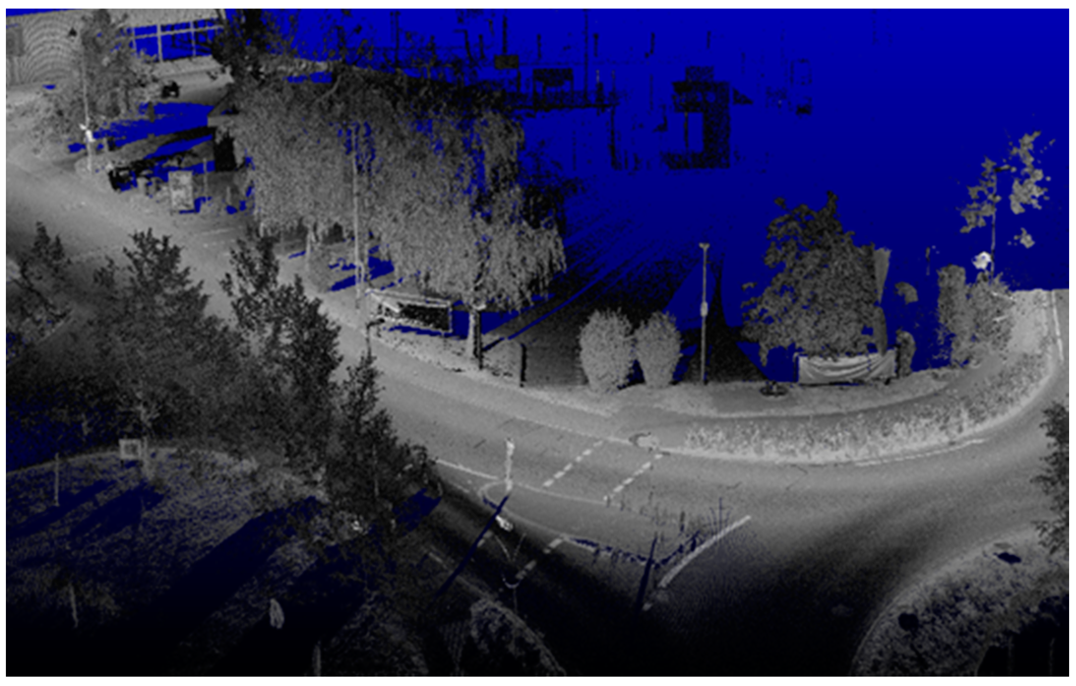
2.1. Mobile Mapping System and Data
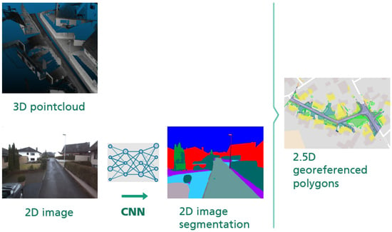
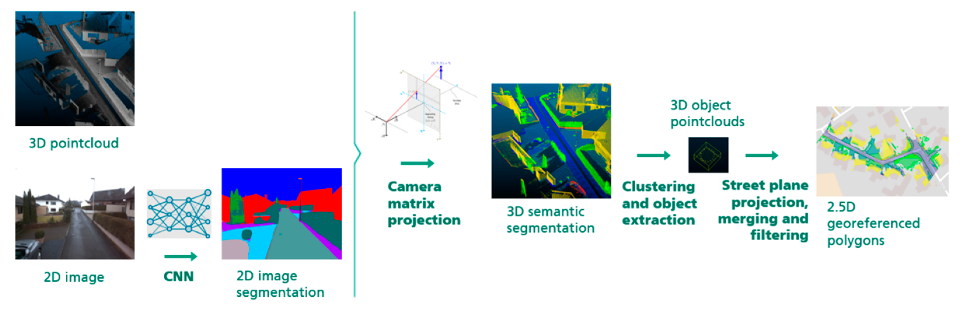
2.2. Processing Pipeline
3. Results
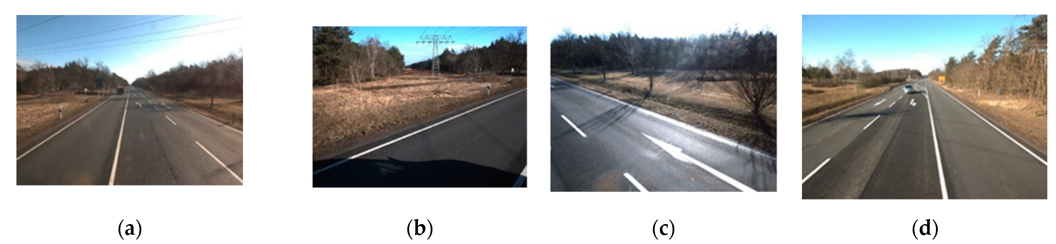
- (a)
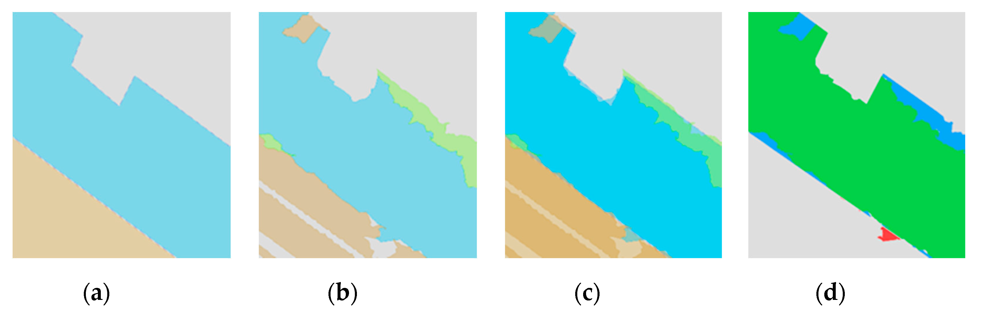
- Surfaces, i.e., areas of ground covered with a specific material (e.g., asphalt or grass; see above). Knowing the exact extent of a surface is important in order to be able to calculate the cost of implementing a planned route though several areas and minimize this cost during the routing process (building through grass is cheaper than opening up pavement). We want to reflect this in our evaluation strategy and compute measures based on area overlap.
- (b)
- Disrupting objects, i.e., objects placed on or inside a surface, which may disrupt a potential broadband route, such as curbstones or rail tracks. The exact area size of these objects is less relevant for the application, since the route planning establishes buffer zones around disrupting objects; however, since undetected “holes” in continuous objects can significantly alter planned routes, high recall is important in the detection of these objects.
3.1. Reference Data Set
3.2. Evaluation
4. Conclusions
Author Contributions
Funding
Acknowledgments
Conflicts of Interest
References
- Son, H.; Bosché, F.; Kim, C. As-built data acquisition and its use in production monitoring and automated layout of civil infrastructure: A survey. Adv. Eng. Inform. 2015, 29, 172–183. [Google Scholar] [CrossRef]
- Walker, J.; Awange, J.L. Surveying for Civil and Mine Engineers. Theory, Workshops, and Practicals; Springer: Cham, Switzerland, 2018; ISBN 9783319531298. [Google Scholar]
- El-Sheimy, N. An overview of mobile mapping systems. In Proceedings of the FIG Working Week 2005 and GSDI-8, Cairo, Egypt, 16–21 April 2005. [Google Scholar]
- Puente, I.; González-Jorge, H.; Martínez-Sánchez, J.; Arias, P. Review of mobile mapping and surveying technologies. Measurement 2013, 46, 2127–2145. [Google Scholar] [CrossRef]
- Jia, Y.; Shelhamer, E.; Donahue, J.; Karayev, S.; Long, J.; Girshick, R.; Guadarrama, S.; Darrell, T. Caffe: Convolutional architecture for fast feature embedding. arXiv 2014, arXiv:1408.5093. [Google Scholar]
- Ma, L.; Li, Y.; Li, J.; Wang, C.; Wang, R.; Chapman, M. Mobile Laser scanned point-clouds for road object detection and extraction: A review. Remote Sens. 2018, 10, 1531. [Google Scholar] [CrossRef]
- Che, E.; Jung, J.; Olsen, M.J. Object recognition, segmentation, and classification of mobile laser scanning point clouds: A state of the art review. Sensors 2019, 19, 810. [Google Scholar] [CrossRef] [PubMed]
- Krizhevsky, A.; Sutskever, I.; Hinton, G.E. ImageNet classification with deep convolutional neural networks. In Advances in Neural Information Processing Systems, Tahoe City, CA, USA, 2012; Curran Associates Inc.: New York, NY, USA, 2012; pp. 1097–1105. [Google Scholar]
- Long, J.; Shelhamer, E.; Darrell, T. Fully convolutional networks for semantic segmentation. In Proceedings of the 2015 IEEE Conference on Computer Vision and Pattern Recognition (CVPR), Boston, MA, USA, 7–12 June 2015; IEEE: Piscataway, NJ, USA, 2015; pp. 3431–3440. ISBN 9781467369640. [Google Scholar]
- Chen, L.-C.; Zhu, Y.; Papandreou, G.; Schroff, F.; Adam, H. Encoder-decoder with atrous separable convolution for semantic image segmentation. arXiv 2018, arXiv:1802.02611. [Google Scholar]
- Maturana, D.; Scherer, S. VoxNet: A 3D convolutional neural network for real-time object recognition. In Proceedings of the 2015 IEEE/RSJ International Conference on Intelligent Robots and Systems (IROS), Hamburg, Germany, 28 September–2 October 2015; pp. 922–928. [Google Scholar]
- Qi, C.R.; Su, H.; Mo, K.; Guibas, L.J. PointNet: Deep learning on point sets for 3D classification and segmentation. arXiv 2016, arXiv:1612.00593. [Google Scholar]
- Ding, Z.; Han, X.; Niethammer, M. VoteNet: A deep learning label fusion method for multi-atlas segmentation. arXiv 2019, arXiv:1904.08963. [Google Scholar]
- Shi, S.; Guo, C.; Jiang, L.; Wang, Z.; Shi, J.; Wang, X.; Li, H. PV-RCNN: Point-voxel feature set abstraction for 3D object detection. arXiv 2019, arXiv:1912.13192. [Google Scholar]
- Guo, Y.; Wang, H.; Hu, Q.; Liu, H.; Liu, L.; Bennamoun, M. Deep learning for 3D point clouds: A survey. arXiv 2019, arXiv:1912.12033. [Google Scholar] [CrossRef]
- Qi, C.R.; Chen, X.; Litany, O.; Guibas, L.J. ImVoteNet: Boosting 3D object detection in point clouds with image votes. arXiv 2020, arXiv:2001.10692. [Google Scholar]
- Zhang, R.; Li, G.; Li, M.; Wang, L. Fusion of images and point clouds for the semantic segmentation of large-scale 3D scenes based on deep learning. ISPRS J. Photogramm. Remote Sens. 2018, 143, 85–96. [Google Scholar] [CrossRef]
- Cordts, M.; Omran, M.; Ramos, S.; Rehfeld, T.; Enzweiler, M.; Benenson, R.; Franke, U.; Roth, S.; Schiele, B. The cityscapes dataset for semantic urban scene understanding. arXiv 2016, arXiv:2001.10692. [Google Scholar]
- Ma, L.; Liu, Y.; Zhang, X.; Ye, Y.; Yin, G.; Johnson, B.A. Deep learning in remote sensing applications: A meta-analysis and review. ISPRS J. Photogramm. Remote Sens. 2019, 152, 166–177. [Google Scholar] [CrossRef]
- Tao, C.V. (Ed.) Advances in Mobile Mapping Technology; Taylor & Francis: London, UK, 2007; ISBN 9780415427234. [Google Scholar]
- Kingma, D.P.; Ba, J. Adam: A method for stochastic optimization. arXiv 2014, arXiv:1412.6980. [Google Scholar]
- Fischler, M.A.; Bolles, R.C. Random sample consensus: A paradigm for model fitting with applications to image analysis and automated cartography. Commun. ACM 1981, 24, 381–395. [Google Scholar] [CrossRef]
- Moreira, A.J.C.; Santos, M.Y. Concave hull: A k-nearest neighbours approach for the computation of the region occupied by a set of points. In GRAPP 2007, Proceedings of the Second International Conference on Computer Graphics Theory and Applications, Barcelona, Spain, 8–11 March 2007; Institute for Systems and Technologies of Information, Control and Communication: Barcelona, Spain, 2007; pp. 61–68. [Google Scholar]


 |  |  |  |  |  |  |  |  | |
|---|---|---|---|---|---|---|---|---|---|
| Object Class | Asphalt | Grass | Curbstone | Small Paving | Hole Cover | Gravel | Large Paving | Rail Tracks | Concrete |
| Appearance Rate | 93% | 80% | 78% | 59% | 44% | 13% | 6% | 4% | 4% |
| True Positives (TP) | Intersection area of output polygons of class A with ground truth polygons of class A |
| False Positives (FP) | Intersection area of output polygons of class A with ground truth polygons of class B, C, … (all classes ≠ A) |
| False Negatives (FN) | Intersection area of ground truth polygons of class A with output polygons of class B, C, … (all classes ≠ A) |
| Object Class | Freiburg (03/18) | Freiburg (07/18) | Bornheim | Total | |||||||||||
|---|---|---|---|---|---|---|---|---|---|---|---|---|---|---|---|
| m² | Pr | Rc | F1 | Pr | Rc | F1 | m² | Pr | Rc | F1 | m² | Pr | Rc | F1 | |
| concrete | 409 | 49% | 78% | 60% | 62% | 65% | 64% | 3972 | 97% | 90% | 93% | 4381 | 92% | 89% | 90% |
| asphalt | 75,852 | 97% | 97% | 97% | 94% | 97% | 95% | 13,965 | 90% | 97% | 93% | 89,818 | 94% | 97% | 96% |
| large paving | 480 | 53% | 47% | 50% | 58% | 83% | 68% | 2089 | 89% | 78% | 83% | 2569 | 81% | 75% | 78% |
| small paving | 11,573 | 88% | 88% | 88% | 89% | 81% | 85% | 5997 | 94% | 95% | 94% | 17,570 | 91% | 89% | 90% |
| grass/dirt | 60,646 | 93% | 94% | 94% | 91% | 97% | 94% | 10,536 | 87% | 97% | 92% | 71,182 | 91% | 96% | 93% |
| gravel | 1820 | 65% | 55% | 60% | 60% | 30% | 40% | 17,585 | 98% | 85% | 91% | 19,405 | 96% | 82% | 88% |
| Object Class | Pr | Rc | F1 |
|---|---|---|---|
| asphalt + concrete | 95% | 97% | 96% |
| paving | 92% | 90% | 91% |
| grass, dirt + gravel | 95% | 95% | 95% |
| Object Class | Majority Label | Nearest Label | Δ |
|---|---|---|---|
| concrete | 89% | 90% | +1% |
| asphalt | 95% | 96% | +1% |
| large paving | 67% | 78% | +11% |
| small paving | 81% | 90% | +9% |
| grass/dirt | 88% | 93% | +5% |
| gravel | 73% | 88% | +15% |
| Pr | Rc | F1 | |
|---|---|---|---|
| Rail Tracks | 98% | 83% | 89% |
| Curbstone | 94% | 87% | 90% |
© 2020 by the authors. Licensee MDPI, Basel, Switzerland. This article is an open access article distributed under the terms and conditions of the Creative Commons Attribution (CC BY) license (http://creativecommons.org/licenses/by/4.0/).
Share and Cite
Reiterer, A.; Wäschle, K.; Störk, D.; Leydecker, A.; Gitzen, N. Fully Automated Segmentation of 2D and 3D Mobile Mapping Data for Reliable Modeling of Surface Structures Using Deep Learning. Remote Sens. 2020, 12, 2530. https://doi.org/10.3390/rs12162530
Reiterer A, Wäschle K, Störk D, Leydecker A, Gitzen N. Fully Automated Segmentation of 2D and 3D Mobile Mapping Data for Reliable Modeling of Surface Structures Using Deep Learning. Remote Sensing. 2020; 12(16):2530. https://doi.org/10.3390/rs12162530
Chicago/Turabian StyleReiterer, Alexander, Katharina Wäschle, Dominik Störk, Achim Leydecker, and Niko Gitzen. 2020. "Fully Automated Segmentation of 2D and 3D Mobile Mapping Data for Reliable Modeling of Surface Structures Using Deep Learning" Remote Sensing 12, no. 16: 2530. https://doi.org/10.3390/rs12162530
APA StyleReiterer, A., Wäschle, K., Störk, D., Leydecker, A., & Gitzen, N. (2020). Fully Automated Segmentation of 2D and 3D Mobile Mapping Data for Reliable Modeling of Surface Structures Using Deep Learning. Remote Sensing, 12(16), 2530. https://doi.org/10.3390/rs12162530