Article

Improved Classification of Urban Trees Using a Widespread Multi-Temporal Aerial Image Dataset

by
Daniel S. W. Katz
1,2,*,
Stuart A. Batterman
1 and
Shannon J. Brines
3
1
School of Public Health, University of Michigan, Ann Arbor, MI 48109, USA
2
Dell Medical School, University of Texas at Austin, Austin, TX 78712, USA
3
School for Environment and Sustainability, University of Michigan, Ann Arbor, MI 48109, USA
*
Author to whom correspondence should be addressed.
Remote Sens. 2020, 12(15), 2475; https://doi.org/10.3390/rs12152475
Submission received: 31 May 2020 / Revised: 18 July 2020 / Accepted: 29 July 2020 / Published: 1 August 2020
(This article belongs to the Special Issue Urban Forest Detection with Remote Sensing)

Abstract

:
Urban tree identification is often limited by the accessibility of remote sensing imagery but has not yet been attempted with the multi-temporal commercial aerial photography that is now widely available. In this study, trees in Detroit, Michigan, USA are identified using eight high resolution red, green, and blue (RGB) aerial images from a commercial vendor and publicly available LiDAR data. Classifications based on these data were compared with classifications based on World View 2 satellite imagery, which is commonly used for this task but also more expensive. An object-based classification approach was used whereby tree canopies were segmented using LiDAR, and a street tree database was used for generating training and testing datasets. Overall accuracy using multi-temporal aerial images and LiDAR was 70%, which was higher than the accuracy achieved with World View 2 imagery and LiDAR (63%). When all data were used, classification accuracy increased to 74%. Taxa identified with high accuracy included Acer platanoides and Gleditsia, and taxa that were identified with good accuracy included Acer, Platanus, Quercus, and Tilia. Our results show that this large catalogue of multi-temporal aerial images can be leveraged for urban tree identification. While classification accuracy rates vary between taxa, the approach demonstrated can have practical value for socially or ecologically important taxa.

Graphical Abstract

1. Introduction

Urban trees provide ecosystem services such as air pollution removal, cooling, and storm water retention as well as ecosystem disservices, including the release of volatile organic compounds and allergenic pollen [1,2]. The services and disservices provided by trees vary substantially between taxa (e.g., [3,4,5]) and they also vary across space [6,7]. Comprehensive maps of urban trees at the species or genus level would be tremendously useful for urban foresters, planners, ecologists, and public health practitioners. For example, maps of ash trees have been used to help manage emerald ash borer outbreaks in urban settings [8,9], and maps of wind-pollinated trees could help to predict allergenic pollen exposure [10].
Most data on urban trees is collected using plot-based sampling methods such as i-Tree Eco [11], and the United States Forest Service has initiated a plot-based survey program in over 100 urban forests [12]. These plot-based sampling approaches provide unbiased city-wide estimates of urban tree composition [11], but do not generate the comprehensive maps of trees that would be most useful for managers and researchers. Surveys of street trees (i.e., city owned trees in the right of way) are common in medium and large cities and often measure all street trees in a city [13,14]. However, street trees are only a small fraction of urban trees (~5–10%; [15,16]) and are not representative of overall forest composition. Thus, there is considerable demand for more comprehensive tree mapping methods.
Remote sensing offers an attractive tool for urban tree classification and this approach has been investigated vigorously. Multi-spectral satellite imagery has been widely used for tree classification; one of the most commonly used satellites is WorldView 2 [17,18,19,20,21,22,23,24], although others are also used, such as WorldView 3 [24], and Quickbird [25]. However, imagery from these satellites is relatively expensive, has limited swath width, and requires image pre-processing (e.g., atmospheric corrections and cloud masking) that is usually done with proprietary software. Although LiDAR has the potential to identify trees by itself, this requires very high-resolution LiDAR (e.g., >10 ppm) and structural differences in trees; publicly available LiDAR is generally ~1 ppm. Urban trees have been successfully classified with hyperspectral imagery [26,27,28,29,30,31]. However, on-demand airborne hyperspectral imaging programs are expensive and existing datasets are sparse. The accessibility, cost, and resolution of remote sensing data remains a major barrier to tree identification in urban areas.
Aerial photography has long been used to classify plants [32,33,34], but previous studies have generally relied on custom-flown missions that are expensive and cover only small areas. A new source of multi-temporal aerial photography is now widely available and very affordable. Specifically, the company Nearmap (100 Bangaroo Ave, Bangaroo, NSW 2000, Australia) is collecting aerial images in most major American, Australian, Canadian, and New Zealand cities several times a year. While this aerial photography is only conducted in visible bands (RGB), in terms of tree identification, the temporal coverage may compensate for lower spectral resolution [34]. Trees that are very similar spectrally during the main growing season can appear distinct during leaf out, flowering, or leaf senescence or taxa can transition between these phenological stages at different times [35]. Despite the depth of the Nearmap imagery catalogue, we have not seen examples of it being used for tree identification. These easily accessible and abundant multi-temporal aerial images may be useful for tree classification in urban areas.
In this study we classify trees using multi-temporal aerial images from Nearmap, publicly available LiDAR, and a street tree inventory in Detroit, Michigan, USA. We compare classification using this new multi-temporal aerial to classifications using World View 2 satellite imagery. A geographic object image analysis (GEOBIA) framework is used with a random forest classifier. Classification accuracy is assessed for each imagery dataset and we discuss both the potential for the Nearmap aerial photography dataset to be used for urban tree identification and use cases for the resulting predictions.

2. Materials and Methods

2.1. Study Area

Detroit, MI, USA (Figure 1) covers 344 km2, of which 21.6% is tree canopy [36]. Several tree genera are common among street trees (dataset described below), including: Acer, Aesculus, Ailanthus, Catalpa, Celtis, Fraxinus, Ginko, Gleditsia, Morus, Platanus, Populus, Pyrus, Quercus, Tilia, and Ulmus. Vegetation cover has increased in large portions of Detroit over the last three decades [37], likely due to afforestation in vacant areas. Two separate municipalities, Highland Park and Hamtramck, are entirely enclosed by Detroit’s municipal boundaries, and are included in this study. Detroit’s annual average precipitation is 940 mm/ year and average temperature is 10.6 °C.

2.2. Data Description: Tree Census

Davey Tree Company surveyed 169,011 street trees from 2011-2016, which was a project undertaken by the Michigan Department of Natural Resources and funded by the USDA Forest Service State and Private Forestry Program. Trees in right of ways were included but trees in parks, on private property, and in Highland Park and Hamtramck were not. Species were identified and tree locations were recorded using meter-accurate GPS. When compared to manually calculated tree canopy centroids from the high-resolution LiDAR dataset (described below) the RMSE was 2.0 m (this included both measurement error and differences between stem locations and tree canopy centers). Tree diameter at breast height (DBH) was also recorded. The most common tree genera were Acer, Gleditsia, Platanus, Ulmus, and Quercus (Table 1).

2.3. Data Description: Remote Sensing Data
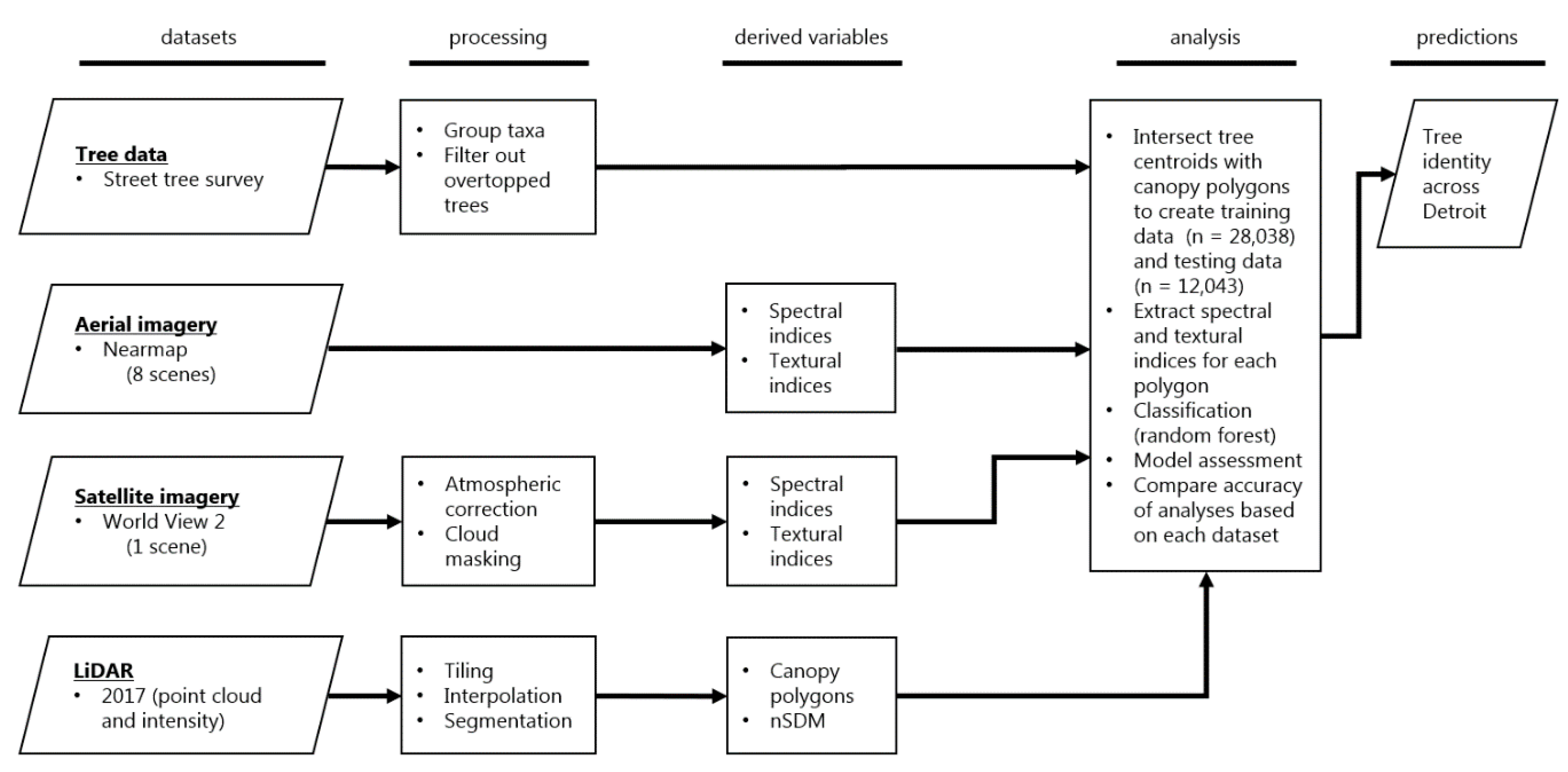
Nearmap (Sydney, Australia) collects high resolution aerial images in 430 urban areas in the United States, which contain 71% of the population. New aerial scenes are collected approximately three times per year in Detroit. (Scenes collected in the winter or that covered only small portions of the study area were omitted from this study.) We used 8 scenes that were collected between 2014 and 2018 (Table 2; image collection dates were: 23 October 2014, 2 November 2014, 1 May 2015, 10 October 2016, 17 April 2017, 23 September 2017, 28 November 2017, and 25 October 2018). These images are available at very high resolution (up to 7.5 cm), but here we used them at a resolution of 0.6 m. Image tiles were downloaded from the Nearmap API, mosaicked, and reprojected to UTM zone 17 N. The average positional accuracy RMSE between the Nearmap scenes was 1.44 m (using an average of 56 control points between each pair of scenes) and the average positional accuracy RMSE compared to LiDAR was 1.06 (Table 2). We also explored aerial images from the National Agricultural Imagery Program but image registration was unsatisfactory.
A World View 2 image taken on 13 June 2011 was obtained from Digital Globe (Table 2). The satellite swath width is 16 km, so we restricted our analysis to that area. Standard atmospheric corrections were applied within Erdas Imagine (Hexagon Geospatial, Madison, AL, USA) and the area with clouds (4.24 km2) was removed from all analyses to ensure fair comparisons between datasets.
LiDAR data have been widely used for tree identification and are now publicly available for much of the United States. In particular, LiDAR can be used to segment tree canopies [31], which replaces the time-consuming task of manually delineating tree crowns that has been undertaken in several studies [17,24,28,29], facilitating GEOBIA approaches on a large spatial scale. We used LiDAR data collected and processed by Sanborn Mapping Company for the State of Michigan, which is now publicly available through the Southeast Michigan Council of Governments. Sanborn Mapping Company collected LiDAR data between 12–23 April 2017, with a Leica ALS70 MPiA LiDAR instrument and an integrated IPAS20 GPS.INS system mounted within an Aero Commander twin engine airplane. Airborne GPS data were postprocessed with Intertial Explorer and LEICA CloudPro and the georeferenced LiDAR data were classified and edited with Terrasolid Terrascan software. Non-vegetated Vertical Accuracy (NVA) was assessed by comparing the digital elevation model with 185 ground control points; the data met Quality Level 2 standards (19.6 cm NVA). Nominal point density was 2.2 points/m2 (Table 2).

2.4. Workflow

The analysis steps are described in Figure 2 and examples of the datasets are shown in Figure 3. LiDAR point cloud data were used to create a pit-free digital surface model (DSM) through a triangulated irregular network approach [38] that included buffering individual points and Gaussian smoothing, implemented within the R package lidR [39]. Other products created included digital elevation models, digital surface models (DSM), and normalized digital surface models (nDSM). Two-dimensional return intensity rasters were provided with the 2017 LiDAR data and were also used in the classification. (See Supplementary Materials).
Tree segmentation of the nDSM was also conducted in lidR. Tree tops were detected by passing a circular local maximum filter over the nDSM raster; the tallest point in the window was assumed to be a tree top. We followed others in assuming that taller trees have larger canopies and therefore varied the local maximum window size as a function of focal pixel height [39,40]. After qualitatively exploring linear and quadratic functions and various parameter values, we selected a linear equation with an intercept of 4.00 and a coefficient of 0.02. Tree crown polygons were then delineated using a seed and region growing algorithm in which each local maximum is considered the seed of a tree crown and neighboring pixels are added to that crown if their heights are less than a certain percentage of the focal pixel’s height; this algorithm is described in detail elsewhere [39,41]. Tree crown polygons that contained more than one street tree point were not used in training or testing data.
To prevent mismatches between points in the street tree database and canopy cover, we discarded trees that were: <10 cm DBH, <5 m tall in 2017, or that may have been under another tree’s canopy (based on manual examination of the data, this was defined as being >12 m tall but having a DBH < 20 cm.) Acer platanoides, the most common tree species, was identified separately from other Acer species, as it is of ecological interest (it is sometimes considered invasive [42]) and spectrally distinct while flowering. Individuals of uncommon genera (<100 individuals in the analysis dataset) were grouped together (“other”) and comprised 0.7% of the dataset.
Several common spectral indices for 3 and 8 band images were calculated [43,44] and are listed in SI 1; for example, for WorldView 2 several measures of NDVI were calculated and for Nearmap images examples of calculated indices included GEI and GRVI [43,44]. The mean, median, and standard deviation of each of these indices were extracted for each tree crown polygon. Similarly, we also extracted the mean, median, and standard deviation from the other available variables, including the original bands from each Nearmap and WorldView 2 image, the LiDAR intensity, and the nSDM. We also explored several textural indices similar to those used by others [24,45] for each dataset using the R package GLCM [46] for pixel windows of size 3, 5, and 9 pixels. However, these derived texture variables contributed little accuracy (<2%) and so we do not include them in the final analysis.
Tree polygons were divided into training data (70%) and testing data (30%) for classification. Classification was conducted using the randomForest package in R [47] based on the remote sensing variables that had been extracted for each polygon. Confusion matrices were computed for testing data. Analyses were conducted using data from all sources (i.e., WorldView 2, Nearmap, and LiDAR data) and then separate analyses were conducted to compare the accuracy of models using different subsets of data (e.g., WorldView 2 vs. Nearmap). Variable importance was measured by the mean decrease in accuracy and Gini values when a variable was omitted from the model. Predictions were created across the study area by extracting data for each segmented polygon that was more than 50% tree cover; creation of that tree cover layer is described elsewhere [36]. Analyses and data exploration were conducted with R 3.5 [48], ArcGIS Desktop 10.7, and ArcGIS Pro 2.4 (ESRI, Redland, CA, USA).

3. Results

3.1. Classification Results

Overall model accuracy reached 74% when all data sources were included (Table 3). Nearmap imagery by itself had an overall accuracy of 68%, whereas WorldView 2 imagery had an accuracy of 58%; when LiDAR-derived metrics (i.e., height and intensity) were also included, accuracy rates rose to 70% for Nearmap imagery rose and to 63% for WorldView 2. Thus, including Nearmap imagery improved tree identification accuracy. User accuracy was far higher than producer accuracy; in the highest accuracy model these were 82% and 38% respectively. The kappa statistic for this model was 0.68.
Classification accuracy for the focal taxa using the model that included all of the datasets (Table 4) was highest for Acer platanoides (92% producer accuracy and 89% user accuracy), and Gleditsia tricanthos (92% and 76%). Other taxa had somewhat lower accuracy, including Platanus (68% and 85%), Acer (84% and 56%), and Catalpa (64% and 92%), Quercus (53% and 83%), Ulmus (34% and 72%), and Tilia (59% and 80%).

3.2. Variable Importance
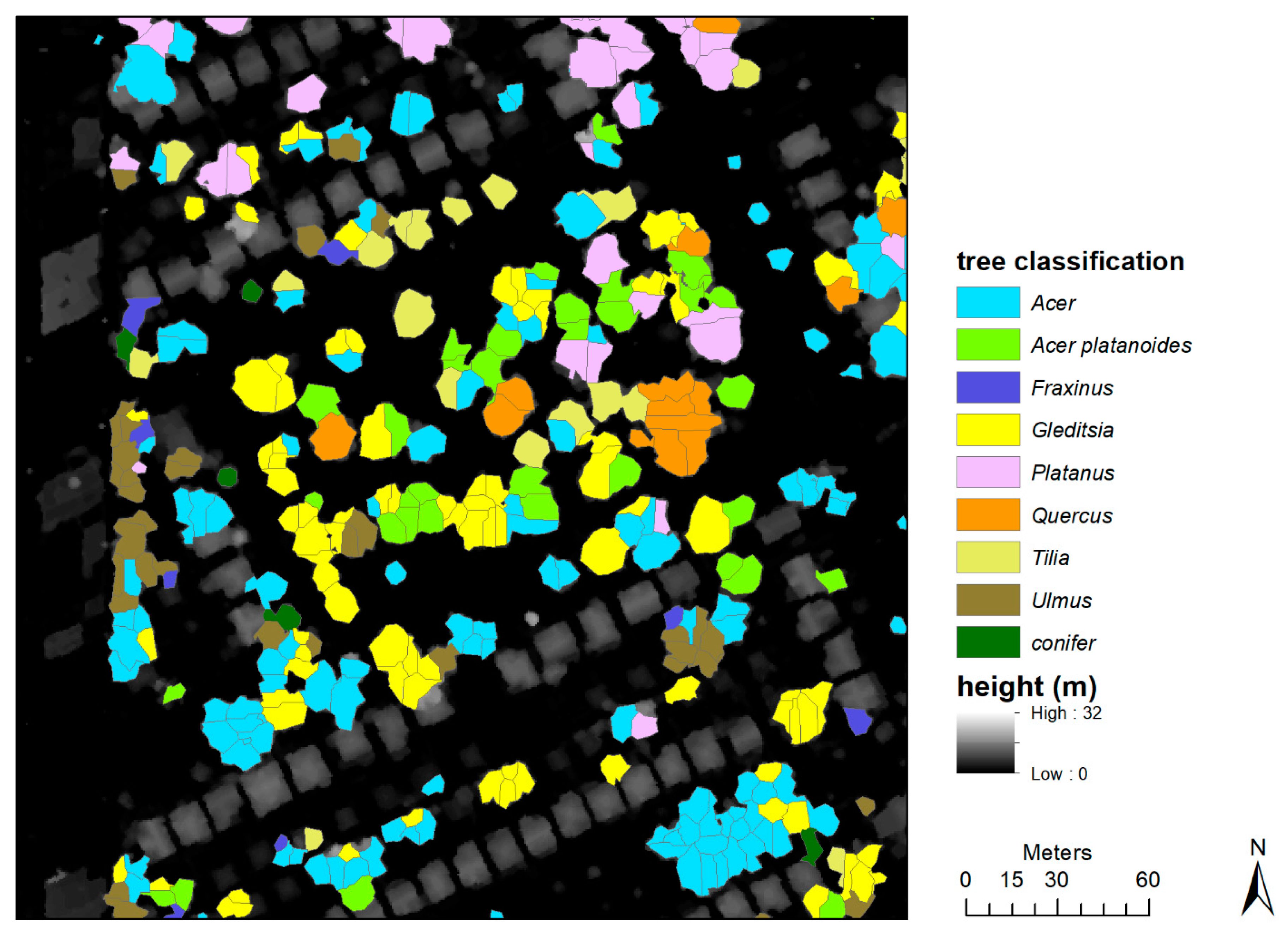
Of the top ten most important variables (defined here by ranking the mean decrease in accuracy when that variable was omitted), eight were from Nearmap and two were from WorldView 2 (SI 2: Variable importance). Mean and median summaries of polygons accounted for three and six of the top ten variables respectively. The top Nearmap indices were gei, grvi, and sgreen (SI 2: Variable importance). The three Nearmap images that were represented in the top ten variables were 25 October 2018, 28 November 2017, and 2 November 2014.

3.3. Predictions

We predicted tree identity for 553,218 polygons across the Detroit study area (Figure 4, Table 5, SI 3). The most commonly predicted taxa were Acer (235,292 polygons), Gleditsia (126,330), Acer platanoides (74,892), and Quercus (29,287 polygons). The predicted relative canopy area of these four taxa were, respectively, 42%, 22%, 14%, and 6%. The other 14 focal taxa were predicted to compose 16% of canopy area.

4. Discussion

4.1. Aerial Images for Tree Classification

Multi-temporal aerial images were useful for urban tree classification and performed better than commonly used WorldView 2 satellite imagery. The Nearmap image catalogue is expanding rapidly and could improve tree identification in urban areas. It is also affordable, scalable, and avoids the need for atmospheric correction and cloud cover masks.
Multi-temporal imagery can increase tree classification accuracy [24,49]. This is likely due to differences in phenology and reflectance that only occur during certain phenological stages (e.g., flowering). For example, Acer platanoides displays distinctive neon green foliage and flowers in early spring, Gleditsia triacanthos has yellow leaves that senesce relatively early in the fall, and Quercus leaves often stay on trees long after other deciduous genera have dropped their leaves. Including more images in an analysis increases the likelihood of observing phenological differences that can aid identification.

4.2. Accuracy Compared to Other Studies

The tree identification accuracy of the model that included LiDAR and aerial images but not satellite imagery (70%) is comparable to other studies of urban trees using satellite imagery. For example, a study of fairly uniformly grown trees in Beijing achieved accuracies of 80–92% using bi-temporal images from WorldView 2 and WorldView 3 and manually delineated tree canopies [24]. A study in Tampa, Florida, USA achieved overall accuracy rates of 56% with WorldView 2 data [22]. Differences in accuracy between studies may also be due to both the amount of spectral and structural similarity between the study taxa and the imagery analyzed. Accuracy is also similar to studies that investigated tree identity in non-urban settings, even though urban areas offer unique challenges such as building shadows and mixed signatures from surfaces beneath trees. For example, studies using WorldView 2 imagery have reported accuracy rates of 30–95% [17], 83% [18], 92% [19], 40–100% [20], 70–90% [50], 67–95% [21], and 65–85% [23].

4.3. Leveraging Urban Tree Censuses

Urban tree databases are becoming increasingly common [13,14] and are often GIS-based. In cases, these have already been leveraged for use in tree identification with remote sensing [26,29]. Study designs that require additional field work, such as manually delineating tree crowns, have been generally limited to relatively small sample sizes [24,28,29]. The larger sample sizes provided by automated extraction of tree polygons from street tree databases allow for larger and more sophisticated models. However, this approach does have several potential limitations: canopy segmentation error, temporal mismatches between street tree surveys and remote sensing data, and records that could impede tree identification (e.g., understory trees that are overtopped by large trees). Street tree databases are also not representative of overall tree composition. In Detroit, several early successional genera, including Ulmus, Populus, and Morus, appear more common among non-street trees (personal observation). This has the potential to bias classification of taxa that are disproportionately common as either street trees or non-street trees. Future studies may be able to address this bias by selecting training or testing datasets that are representative of the area’s tree composition, for example by consulting data from the Urban Forest Inventory and Analysis program, which will be available soon. Despite the challenges and limitations inherent in leveraging street tree data, this approach can yield predictions with real value.

4.4. Applications

The usefulness of the predictions generated will largely depend on whether the well-identified taxa are of importance, e.g., through the provisioning of ecosystem services or disservices. For example, Quercus (user accuracy: 0.83) canopy cover was predicted to vary considerably throughout the city, and these cover estimates are highly effective for predicting neighborhood-level differences in airborne Quercus pollen (manuscript in preparation), which is both extensive and of considerable interest to those with pollen allergies [10]. These predictions could also be useful for guiding future responses to host-specific tree pests and pathogens or for understanding the spread of potentially invasive species, such as Acer platanoides (user accuracy: 0.89) in to natural areas. However, prediction accuracy for many rare tree genera (i.e., Aesculus, Ailanthus, Celtis, Ginko, Populus, and Morus) were poor, thus these predictions should not be used to assess urban tree diversity.

4.5. Limitations

Spatial misalignment can interfere with combining multiple data sources in a single analysis [51]. In the present study, the average RMSEs for the aerial and satellite imagery compared to the LiDAR data were both low (1.62 and 1.06 m), especially compared to the average size of classified polygons (71 m2). A GEOBIA approach may have helped to reduce the effect of minor misalignment of datasets in this analysis; preliminary analyses at the pixel level returned accuracies <50% (data not shown). Use of object-based approach in urban environments using LiDAR is a rapidly increasing [52], and so registration errors may be less of a barrier for data fusion in future studies. A challenge for applying GEOBIA approaches to tree identification in urban areas is that individual tree segmentation still is usually inaccurate [53], especially when there are many types of trees growing in different conditions and when trees have intermingled canopies and irregular forms [52]. The resulting polygons may sometimes not include an entire individual tree (i.e., over segmentation), but this is not problematic if each polygon is large enough to have sufficient information for tree identification and if the predictions are used at the stand level (e.g., for calculating total canopy area per taxon). A limitation of our reliance on previously collected datasets is that we did not have manually delineated tree canopies available to quantitatively assess the accuracy of the segmentation algorithm; this limitation is shared by most application-oriented uses of tree segmentation algorithms [52].
One potential limitation associated with using phenological signals to identify plants is the variability of phenology, even within a city. For example, we found that the range of peak flowering times for oak trees within Detroit varied by several weeks [54]. The usefulness of phenological signals to identify plants will be limited when images encompass that variation. Most cities contain thermal gradients [55,56] that affect phenology [57,58] and future studies would do well to consider this when conducting analyses that depend on phenological differences.

5. Conclusions

This study shows that common commercially available multi-temporal aerial images can improve classification of urban trees. Predictions using both aerial images and LiDAR had an overall accuracy of 70% whereas predictions using LiDAR and World View 2 imagery had an accuracy of 63%. Including both aerial images and satellite imagery increased accuracy to 74%. These results highlight the benefits of adding widespread aerial photography to urban tree identification analyses and showcase some practical uses for the prediction of well-identified taxa across the study area.

Supplementary Materials

The following are available online at https://www.mdpi.com/2072-4292/12/15/2475/s1, Supporting Information 1: Derived spectral and texture variables; Supporting Information 2: Table of most important variables; Supporting Information 3: Shapefile of predicted tree identity.

Author Contributions

Conceptualization, D.S.W.K. and S.A.B.; data assembly and processing, D.S.W.K. and S.J.B.; pixel-based analysis S.J.B., GEOBIA analysis, D.S.W.K., writing, D.S.W.K. and S.A.B. All authors have read and agreed to the published version of the manuscript.

Funding

Daniel S. W. Katz was supported by the National Institute of Environmental Health Sciences through a NRSA postdoctoral fellowship (Grant Number F32 ES026477 and by the Michigan Institute for Clinical Health Research through the Postdoctoral Translational Scholars Program (Grant Number UL1 TR002240). Stuart A. Batterman also acknowledges support from grant P30 ES017885 from the National Institute of Environmental Health Sciences, National Institutes of Health. The content is solely the responsibility of the authors and does not necessarily represent the official views of the National Institutes of Health. Purchase of World View 2 imagery was supported by the Clark Library through a data acquisition grant; access to Nearmap imagery was also provided by the Clark Library.

Acknowledgments

We thank Todd Mistor (City of Detroit municipal forester), Josh Behounek and Lee Mueller (Davey Tree Company), and Kevin Sayers (Michigan Department of Natural Resources) for providing the tree survey data. We also thank Everett Root for providing us with an early copy of the 2017 LiDAR data. We also thank Kelly McManus for help on early stages of this project and Kathleen Bergen for remote sensing advice.

Conflicts of Interest

The authors declare no conflict of interest.

References

  1. Roy, S.; Byrne, J.; Pickering, C. A systematic quantitative review of urban tree benefits, costs, and assessment methods across cities in different climatic zones. Urban For. Urban Green. 2012, 11, 351–363. [Google Scholar] [CrossRef] [Green Version]
  2. Eisenman, T.S.; Churkina, G.; Jariwala, S.P.; Kumar, P.; Lovasi, G.S.; Pataki, D.E.; Weinberger, K.R.; Whitlow, T.H.; Eisenman, T.S.; Churkina, G.; et al. Urban trees, air quality, and asthma: An interdisciplinary review. Landsc. Urban Plan. 2019, 187, 47–59. [Google Scholar] [CrossRef]
  3. Sæbø, A.; Popek, R.; Nawrot, B.; Hanslin, H.M.; Gawronska, H.; Gawronski, S.W. Plant species differences in particulate matter accumulation on leaf surfaces. Sci. Total Environ. 2012, 427–428, 347–354. [Google Scholar] [CrossRef] [PubMed]
  4. Yang, J.; Chang, Y.; Yan, P. Ranking the suitability of common urban tree species for controlling PM 2.5 pollution. Atmos. Pollut. Res. 2014, 6, 267–277. [Google Scholar] [CrossRef] [Green Version]
  5. Green, B.J.; Levetin, E.; Horner, W.E.; Codina, R.; Barnes, C.S.; Filley, W.V. Landscape Plant Selection Criteria for the Allergic Patient. J. Allergy Clin. Immunol. Pract. 2018, 6, 1869–1876. [Google Scholar] [CrossRef]
  6. Pulighe, G.; Fava, F.; Lupia, F. Insights and opportunities from mapping ecosystem services of urban green spaces and potentials in planning. Ecosyst. Serv. 2016, 22, 1–10. [Google Scholar] [CrossRef]
  7. Bodnaruk, E.W.; Kroll, C.N.; Yang, Y.; Hirabayashi, S.; Nowak, D.J.; Endreny, T.A. Where to plant urban trees? A spatially explicit methodology to explore ecosystem service tradeoffs. Landsc. Urban Plan. 2017, 157, 457–467. [Google Scholar] [CrossRef] [Green Version]
  8. Pontius, J.; Hanavan, R.P.; Hallett, R.A.; Cook, B.D.; Corp, L.A. High spatial resolution spectral unmixing for mapping ash species across a complex urban environment. Remote Sens. Environ. 2017, 199, 360–369. [Google Scholar] [CrossRef]
  9. Souci, J.; Hanou, I.; Puchalski, D. High-resolution remote sensing image analysis for early detection and response planning for emerald ash borer. Photogramm. Eng. Remote Sens. 2009, 75, 905–909. [Google Scholar]
  10. Katz, D.S.W.; Batterman, S.A. Urban-scale variation in pollen concentrations: A single station is insufficient to characterize daily exposure. Aerobiologia 2020. [Google Scholar] [CrossRef]
  11. Nowak, D.J.; Crane, D.E.; Stevens, J.C.; Hoehn, R.E.; Walton, J.T.; Bond, J. A ground-based method of assessing urban forest structure and ecosystem services. Arboric. Urban For. 2008, 34, 347–358. [Google Scholar]
  12. US Forest Service. Urban Forest Inventory & Analysis. Available online: https://www.fia.fs.fed.us/program-features/urban/ (accessed on 1 January 2020).
  13. Keller, J.K.K.; Konijnendijk, C.C. Short communication: A comparative analysis of municipal urban tree inventories of selected major cities in North America and Europe. Arboric. Urban For. 2012, 38, 24–30. [Google Scholar]
  14. Hauer, R.J.; Peterson, W.D. Municipal Tree Care and Management in the United States: A 2014 Urban and Community Forestry Census of Tree Activities; Special Publication 16-1; College of Natural Resources, University of Wisconsin: Stevens Point, WI, USA, 2016. [Google Scholar]
  15. McPherson, E.G.; Nowak, D.J.; Heisler, G.; Grimmond, S.; Souch, C.; Grant, R.; Rowntree, R. Quantifying urban forest structure, function, and value: The Chicago Urban Forest Climate Project. Urban Ecosyst. 1997, 1, 49–61. [Google Scholar] [CrossRef]
  16. McPherson, E.G.; Van Doorn, N.S.; Peper, P.J. Urban Tree Database and Allometric Equations (General technical report PSW-GTR-253); U.S. Department of Agriculture, Forest Service, Pacific Southwest Research Station: Albany, CA, USA, 2016; Available online: https://www.fs.fed.us/psw/publications/documents/psw_gtr253/psw_gtr_253.pdf (accessed on 1 January 2020).
  17. Immitzer, M.; Atzberger, C.; Koukal, T. Tree species classification with Random forest using very high spatial resolution 8-band worldView-2 satellite data. Remote Sens. 2012, 4, 2661–2693. [Google Scholar] [CrossRef] [Green Version]
  18. Waser, L.T.; Küchler, M.; Jütte, K.; Stampfer, T. Evaluating the potential of worldview-2 data to classify tree species and different levels of ash mortality. Remote Sens. 2014, 6, 4515–4545. [Google Scholar] [CrossRef] [Green Version]
  19. Cho, M.A.; Malahlela, O.; Ramoelo, A. Assessing the utility WorldView-2 imagery for tree species mapping in South African subtropical humid forest and the conservation implications: Dukuduku forest patch as case study. Int. J. Appl. Earth Obs. Geoinf. 2015, 38, 349–357. [Google Scholar] [CrossRef]
  20. Karna, Y.K.; Hussin, Y.A.; Gilani, H.; Bronsveld, M.C.; Murthy, M.S.R.; Qamer, F.M.; Karky, B.S.; Bhattarai, T.; Aigong, X.; Baniya, C.B. Integration of WorldView-2 and airborne LiDAR data for tree species level carbon stock mapping in Kayar Khola watershed, Nepal. Int. J. Appl. Earth Obs. Geoinf. 2015, 38, 280–291. [Google Scholar] [CrossRef]
  21. Deng, S.; Katoh, M.; Guan, Q.; Yin, N.; Li, M. Interpretation of forest resources at the individual tree level at Purple Mountain, Nanjing City, China, using WorldView-2 imagery by combining GPS, RS and GIS technologies. Remote Sens. 2013, 6, 87–110. [Google Scholar] [CrossRef] [Green Version]
  22. Pu, R.; Landry, S. A comparative analysis of high spatial resolution IKONOS and WorldView-2 imagery for mapping urban tree species. Remote Sens. Environ. 2012, 124, 516–533. [Google Scholar] [CrossRef]
  23. Omer, G.; Mutanga, O.; Abdel-Rahman, E.M.; Adam, E. Performance of Support Vector Machines and Artifical Neural Network for Mapping Endangered Tree Species Using WorldView-2 Data in Dukuduku Forest, South Africa. IEEE J. Sel. Top. Appl. Earth Obs. Remote Sens. 2015, 8, 4825–4840. [Google Scholar] [CrossRef]
  24. Li, D.; Ke, Y.; Gong, H.; Li, X. Object-Based Urban Tree Species Classification Using Bi-Temporal WorldView-2 and WorldView-3 Images. Remote Sens. 2015, 7, 16917–16937. [Google Scholar] [CrossRef] [Green Version]
  25. Ardila, J.P.; Bijker, W.; Tolpekin, V.A.; Stein, A. Context-sensitive extraction of tree crown objects in urban areas using VHR satellite images. Int. J. Appl. Earth Obs. Geoinf. 2012, 15, 57–69. [Google Scholar] [CrossRef] [Green Version]
  26. Alonzo, M.; Bookhagen, B.; Roberts, D.A. Urban tree species mapping using hyperspectral and lidar data fusion. Remote Sens. Environ. 2014, 148, 70–83. [Google Scholar] [CrossRef]
  27. Voss, M.; Sugumaran, R. Seasonal effect on tree species classification in an urban environment using hyperspectral data, LiDAR, and an object-oriented approach. Sensors 2008, 8, 3020–3036. [Google Scholar] [CrossRef] [PubMed] [Green Version]
  28. Jensen, R.R.; Hardin, P.J.; Hardin, A.J. Classification of urban tree species using hyperspectral imagery. Geocarto Int. 2012, 27, 443–458. [Google Scholar] [CrossRef]
  29. Liu, L.; Coops, N.C.; Aven, N.W.; Pang, Y. Mapping urban tree species using integrated airborne hyperspectral and LiDAR remote sensing data. Remote Sens. Environ. 2017, 200, 170–182. [Google Scholar] [CrossRef]
  30. Zhang, C.; Qiu, F. Mapping Individual Tree Species in an Urban Forest Using Airborne Lidar Data and Hyperspectral Imagery. Photogramm. Eng. Remote Sens. 2012, 78, 1079–1087. [Google Scholar] [CrossRef] [Green Version]
  31. Zhang, Z.; Kazakova, A.; Moskal, L.M.; Styers, D.M. Object-based tree species classification in urban ecosystems using LiDAR and hyperspectral data. Forests 2016, 7, 122. [Google Scholar] [CrossRef] [Green Version]
  32. Hershey, R.; Befort, W. Aerial Photo Guide to New England Forest Types (General Technical Report NE-195); U.S. Department of Agriculture, Forest Service, Northeastern Forest Experiment Station: Washington, DC, USA, 1995. Available online: https://www.nrs.fs.fed.us/pubs/6667 (accessed on 1 January 2020).
  33. Morgan, J.L.; Gergel, S.E.; Coops, N.C. Aerial Photography: A Rapidly Evolving Tool for Ecological Management. Bioscience 2010, 60, 47–59. [Google Scholar] [CrossRef]
  34. Key, T.; Warner, T.A.; Mcgraw, J.B.; Fajvan, M.A. A Comparison of Multispectral and Multitemporal Information in High Spatial Resolution Imagery for Classification of Individual Tree Species in a Temperate Hardwood Forest. Remote Sens. Environ. 2001, 75, 100–112. [Google Scholar] [CrossRef]
  35. Polgar, C.A.; Primack, R.B. Leaf-out phenology of temperate woody plants: From trees to ecosystems. New Phytol. 2011, 191, 926–941. [Google Scholar] [CrossRef] [PubMed]
  36. Katz, D.S.W.; Batterman, S.A. Allergenic pollen production across a large city for common ragweed (Ambrosia artemisiifolia). Landsc. Urban Plan. 2019, 190, 103615. [Google Scholar] [CrossRef]
  37. Endsley, K.A.; Brown, D.G.; Bruch, E. Housing Market Activity is Associated with Disparities in Urban and Metropolitan Vegetation. Ecosystems 2018, 21, 1–15. [Google Scholar] [CrossRef]
  38. Khosravipour, A.; Skidmore, A.K.; Isenburg, M.; Wang, T.; Hussin, Y.A. Generating pit-free canopy height models from airborne LiDAR. Photogramm. Eng. Remote Sens. 2014, 80, 863–872. [Google Scholar] [CrossRef]
  39. Roussel, J.; Auty, D. Lidr: Airborne Lidar Data Manipulation and Visualization for Forestry Applications. 2017. Available online: https://github.com/Jean-Romain/lidR (accessed on 1 January 2020).
  40. Popescu, S.C.; Wynne, R.H. Seeing the Trees in the Forest: Using Lidar and Multispectral Data Fusion with Local Filtering and Variable Window Size for Estimating Tree Height. Photogramm. Eng. Remote Sens. 2004, 70, 589–604. [Google Scholar] [CrossRef] [Green Version]
  41. Dalponte, M.; Coomes, D.A. Tree-centric mapping of forest carbon density from airborne laser scanning and hyperspectral data. Methods Ecol. Evol. 2016, 1236–1245. [Google Scholar] [CrossRef] [Green Version]
  42. Martin, P.H.; Marks, P.L. Intact forests provide only weak resistance to a shade-tolerant invasive Norway maple (Acer platanoides L.). J. Ecol. 2006, 94, 1070–1079. [Google Scholar] [CrossRef]
  43. Mizunuma, T.; Mencuccini, M.; Wingate, L.; Ogée, J.; Nichol, C.; Grace, J. Sensitivity of colour indices for discriminating leaf colours from digital photographs. Methods Ecol. Evol. 2014, 5, 1078–1085. [Google Scholar] [CrossRef] [Green Version]
  44. Weil, G.; Lensky, I.M.; Resheff, Y.S.; Levin, N. Optimizing the timing of unmanned aerial vehicle image acquisition for applied mapping ofwoody vegetation species using feature selection. Remote Sens. 2017, 9, 1130. [Google Scholar] [CrossRef] [Green Version]
  45. Heinzel, J.; Koch, B. Investigating multiple data sources for tree species classification in temperate forest and use for single tree delineation. Int. J. Appl. Earth Obs. Geoinf. 2012, 18, 101–110. [Google Scholar] [CrossRef]
  46. Zvoleff, A. GLCM: Calculate Textures from Grey-Level Co-Occurrence Matrices (GLCMs). 2016. Available online: https://CRAN.R-project.org/package=glcm (accessed on 1 January 2020).
  47. Liaw, A.; Wiener, M. Classification and Regression by randomForest. R news 2002, 2, 18–22. [Google Scholar] [CrossRef]
  48. R Core Team R: A Language and Environment for Statistical Computing. R Foundation for Statistical Computing: Vienna, Austria, 2018. Available online: www.R-project.org (accessed on 1 January 2020).
  49. Hill, R.A.; Wilson, A.K.; George, M.; Hinsley, S.A. Mapping tree species in temperate deciduous woodland using time-series multi-spectral data. Appl. Veg. Sci. 2010, 13, 86–99. [Google Scholar] [CrossRef]
  50. Heenkenda, M.K.; Joyce, K.E.; Maier, S.W.; Bartolo, R. Mangrove species identification: Comparing WorldView-2 with aerial photographs. Remote Sens. 2014, 6, 6064–6088. [Google Scholar] [CrossRef] [Green Version]
  51. Wang, K.; Wang, T.; Liu, X. A review: Individual tree species classification using integrated airborne LiDAR and optical imagery with a focus on the urban environment. Forests 2019, 10, 1. [Google Scholar] [CrossRef] [Green Version]
  52. Zhen, Z.; Quackenbush, L.J.; Zhang, L. Trends in automatic individual tree crown detection and delineation-evolution of LiDAR data. Remote Sens. 2016, 8, 333. [Google Scholar] [CrossRef] [Green Version]
  53. Marconi, S.; Graves, S.J.; Gong, D.; Nia, M.S.; Le Bras, M.; Dorr, B.J.; Fontana, P.; Gearhart, J.; Greenberg, C.; Harris, D.J.; et al. A data science challenge for converting airborne remote sensing data into ecological information. PeerJ 2019, 6, 1–27. [Google Scholar] [CrossRef] [Green Version]
  54. Katz, D.S.W.; Dzul, A.; Kendel, A.; Batterman, S.A. Effect of intra-urban temperature variation on tree flowering phenology, airborne pollen, and measurement error in epidemiological studies of allergenic pollen. Sci. Total Environ. 2019, 653, 1213–1222. [Google Scholar] [CrossRef]
  55. Imhoff, M.L.; Zhang, P.; Wolfe, R.E.; Bounoua, L. Remote sensing of the urban heat island effect across biomes in the continental USA. Remote Sens. Environ. 2010, 114, 504–513. [Google Scholar] [CrossRef] [Green Version]
  56. Rizwan, A.M.; Dennis, L.Y.C.; Liu, C. A review on the generation, determination and mitigation of urban heat island. J. Environ. Sci. 2008, 20, 120–128. [Google Scholar] [CrossRef]
  57. Jochner, S.; Menzel, A. Urban phenological studies—Past, present, future. Environ. Pollut. 2015, 203, 250–261. [Google Scholar] [CrossRef]
  58. Neil, K.; Wu, J. Effects of urbanization on plant flowering phenology: A review. Urban Ecosyst. 2006, 9, 243–257. [Google Scholar] [CrossRef]
Figure 1. Study area including WorldView 2 satellite swath (light blue), the boundary of Detroit (black) and tree cover (green).
Remotesensing 12 02475 g001
Figure 2. Tree identification work flow from input datasets and data processing steps to derived variables and analysis steps.
Remotesensing 12 02475 g002
Figure 3. Input datasets (A) Tree mask (green) and street trees (blue circles), (B) LiDAR derived nSDM and segmented tree canopy objects (blue lines), (C) LiDAR intensity, (D) WorldView 2 RGB image, (E) WorldView 2 panchromatic image, (F) Nearmap image from May 2015, (G) Nearmap image from September 2017, and (H) Nearmap image from November 2017.
Remotesensing 12 02475 g003
Figure 4. Predicted tree identity (colored polygons) and height (nSDM) for the area surrounding Figure 3.
Remotesensing 12 02475 g004
Table 1. Abundant tree taxa in Detroit (>0.02% of relative basal area). This table is based on street trees and does not include trees on private property or in parks. Acer platanoides is included separately from Acer because it is the most abundant species and has distinct life-history characteristics.
Focal TaxaCommon NameAbundant Anemophilous SpeciesRelative Basal Area Street Trees (%)n
AcermapleA. saccharinum, A. rubrum, A. saccharum, A. negundo35.538,363
Acer platanoidesNorway mapleA. platanoides11.430,845
Aesculushorse chestnutA. hippocastanum0.91167
Ailanthustree of heavenA. altissima0.4962
CatalpacatalpaC. speciosa1.61280
CeltishackberryC. occidentalis1.32240
FraxinusashF. Pennsylvanica, F. americana5.211,786
GinkgoginkgoG. biloba0.21122
Gleditsiahoney locustGleditsia tricanthos10.222,331
MorusmulberryM. alba, M. rubra0.42237
Platanussycamore, London planetreeP. occidentalis,
P. x acerfolia
9.112,499
PopuluspoplarP. deltoides, P. alba2.01086
PyruspearP. calleryana0.32644
QuercusoakQ. palustris, Q. rubra, Q. macrocarpa, Q. alba, Q. robur5.66846
TiliabasswoodC. americana, C. cordata3.78144
UlmuselmU. pumila, U. americana, U. rubra10.49989
other-14.842,581
total100169,011
Table 2. Description of remote sensing data including satellite imagery (WorldView 2), aerial images (Nearmap), and LiDAR. Imagery RMSE is calculated in reference to the Lidar (which has a stated RMSE of 17 cm); for the Nearmap image, this is calculated for one image and then other Nearmap images are compared to it.
DatasetScenes (n)YearsSpatial ResolutionSpectral ResolutionRMSE (m)Accessibility
WorldView-2120110.5 m (panchromatic)
2.0 m (multispectral)
1
8
1.62Private; purchase of individual scenes
Nearmap82014–20180.6 m31.06Private; subscription based
LiDAR120172.2 ppm--Public
Table 3. Model diagnostic statistics for different datasets. Model accuracy gives the percent of observations that were predicted correctly, average user accuracy and producer accuracy are averaged across all included taxa.
Model NameAccuracyUser AccuracyProducer AccuracyKappa Statistic
All datasets0.7400.8170.3770.682
LiDAR (all)0.4430.1950.1430.309
LiDAR (intensity only)0.3710.1070.1050.217
LiDAR (all) and Nearmap0.6970.7780.3270.630
LiDAR (all) and WorldView 2 (all)0.6310.6500.2920.548
Nearmap 0.6820.7590.3160.612
WorldView 2 (all)0.5780.5020.2340.479
WorldView 2 (spectral indices)0.5250.4840.2150.414
WorldView 2 (raw)0.5620.4870.2210.459
Table 4. Confusion matrix for model testing dataset. Column are reference data and rows are predicted values. User and producer accuracy are also provided for each group.
AcerAcer platanoidesAesculusAilanthusCatalpaCeltisConiferousFraxinusGinkgoGleditsiaMorusOtherPlatanusPopulusPyrusQuercusTiliaUlmusTotalUser Accuracy
Acer210518236372827913741130246124357211909930037270.56
Acer platanoides1332555482062101822181712203028660.89
Aesculus1123000010101000000280.82
Ailanthus00000000000000000000.00
Catalpa0000660000300000300720.92
Celtis00000000000000000000.00
coniferous0000001720003000001230.74
Fraxinus21717176035003311353317144890.72
Ginkgo00000000000000000000.00
Gleditsia11515131149515622194101942111097696628750.76
Morus00000000000000000000.00
other00000000000100000011.00
Platanus444010206192368720067138050.85
Populus00000000000000000000.00
Pyrus0000000000000013000131.00
Quercus19910010001119603359674320.83
Tilia18121010101006132011131733960.80
Ulmus383001002002031432112283160.72
Total24942788148431039233692452397411251005976068253666212,043
Producer accuracy0.840.920.160.00.640.00.520.510.00.920.00.010.680.00.220.530.590.34
Table 5. Total number of predicted trees (segmented tree canopies) and area for each taxon.
TaxonTrees (n)Trees (%)Area (m2)Area (%)
Acer235,29242.512,770,22442.2
Acer platanoides74,89213.54,250,87214.1
Aesculus9340.253,2200.2
Ailanthus110<0.16486<0.1
Catalpa39260.7185,3730.6
Celtis191<0.112,618<0.1
conifers57571.0290,1761.0
Fraxinus18,3783.3792,8872.6
Ginko96<0.14927<0.1
Gleditsia126,33022.86,615,29521.9
Morus130<0.18431<0.1
other369<0.120,4610.1
Platanus16,3122.9974,6513.2
Populus251<0.116,793<0.1
Pyrus5140.129,022<0.1
Quercus29,2875.31,850,5396.1
Tilia13,2222.4778,3612.6
Ulmus27,2274.91,585,6385.2
Total553,218100.030,245,974100.0

