Article

Assessment of Intra-Annual and Inter-Annual Variabilities of Soil Erosion in Crete Island (Greece) by Incorporating the Dynamic “Nature” of R and C-Factors in RUSLE Modeling

by
Christos Polykretis
1,2,*,
Dimitrios D. Alexakis
1,2,
Manolis G. Grillakis
1,2 and
Stelios Manoudakis
2
1
Lab of Geophysical-Satellite Remote Sensing and Archaeo-Environment, Institute for Mediterranean Studies, Foundation for Research and Technology-Hellas, 74100 Rethymno, Greece
2
School of Environmental Engineering, Technical University of Crete, 73100 Chania, Greece
*
Author to whom correspondence should be addressed.
Remote Sens. 2020, 12(15), 2439; https://doi.org/10.3390/rs12152439
Submission received: 22 June 2020 / Revised: 17 July 2020 / Accepted: 28 July 2020 / Published: 29 July 2020
(This article belongs to the Special Issue Remote Sensing of Soil Erosion)

Abstract

:
Under the continuously changing conditions of the environment, the exploration of spatial variability of soil erosion at a sub-annual temporal resolution, as well as the identification of high-soil loss time periods and areas, are crucial for implementing mitigation and land management interventions. The main objective of this study was to estimate the monthly and seasonal soil loss rates by water-induced soil erosion in Greek island of Crete for two recent hydrologically contrasting years, 2016 (dry) and 2019 (wet), as a result of Revised Universal Soil Loss Equation (RUSLE) modeling. The impact of temporal variability of the two dynamic RUSLE factors, namely rainfall erosivity (R) and cover management (C), was explored by using rainfall and remotely sensed vegetation data time-series of high temporal resolution. Soil, topographical, and land use/cover data were exploited to represent the other three static RUSLE factors, namely soil erodibility (K), slope length and steepness (LS) and support practice (P). The estimated rates were mapped presenting the spatio-temporal distribution of soil loss for the study area on a both intra-annual and inter-annual basis. The identification of high-loss months/seasons and areas in the island was achieved by these maps. Autumn (about 35 t ha−1) with October (about 61 t ha−1) in 2016, and winter (about 96 t ha−1) with February (146 t ha−1) in 2019 presented the highest mean soil loss rates on a seasonal and monthly, respectively, basis. Summer (0.22–0.25 t ha−1), with its including months, showed the lowest rates in both examined years. The intense monthly fluctuations of R-factor were found to be more influential on water-induced soil erosion than the more stabilized tendency of C-factor. In both years, olive groves in terms of agricultural land use and Chania prefecture in terms of administrative division, were detected as the most prone spatial units to erosion.

Graphical Abstract

1. Introduction

Soil erosion is a major environmental process which involves the detachment, transport and accumulation of soil particles from a given initial area to a new depositional area [1]. Despite the fact that its occurrence is affected by anthropogenic activities (e.g., urban expansion, infrastructure development, removal of vegetative coverage and uncontrolled land cultivation), natural driving forces, such as the water and wind, are considered as the main triggers. Among them, water is considered the most important [2]. Soil erosion by water is a gravity-driven process wherein the rainfall and/or surface water initially causes the detachment of soil particles (soil loss). Then, the water moves off down the slope in the form of runoff resulting to the deposition of detached particles downstream (sedimentation).
Due to the serious environmental and economic effects caused by the phases of soil loss and sedimentation, soil erosion has been addressed as one of the most severe natural threats worldwide. Being both “on-site” and “off-site”, these effects are mainly related to soil degradation and ecological environment deterioration. Particularly, the change in physical and chemical characteristics of initial area’s soil, represented by a reduction or loss of its nutrients and organic matter, diminishes the soil fertility and thus the potential agricultural productivity (“on-site” effects). Furthermore, the eutrophication of depositional area’s water resources due to the sedimentation of nutrients, such as nitrogen, phosphorus, potassium, and other pollutants, into the drainage network and water reservoirs leads to an increased pollution of ecosystems (“off-site” effect) [3].
The above possible effects seriously threatening both natural and anthropogenic environments highlight the assessment of the intensity and spatial distribution of soil erosion as a critical need. These assessments constitute the key to quantitatively estimate soil loss and identify areas of high risk. The advances in Geoinformatics technologies, such as geographic information systems (GIS) and remote sensing, as well as the wide spreading of availability of high-quality geospatial data, have facilitated the modeling of soil erosion enabling the quantitative estimation and spatial identification of soil loss. Since the 1930s, but mainly after 1960, several models have been developed to estimate soil loss at different spatial scales [4]. In terms of their complexity, input data requirements and processing, these models range from relatively simple empirical to more complicated conceptual and physical models. In general, the parameters analyzed in conceptual models [5,6] show limited scope for interpreting the process of soil erosion, while physical models [7,8] are more complex requiring barely obtainable, detailed data (e.g., infiltration rates and saturated hydraulic conductivity) [9]. Due to their simplicity and less computational requirements, empirical models have overtaken conceptual and physical models over the recent years [10,11].
In the majority of empirical models, data representing the soil erosion-influencing conditions of a given region like its climate, topography, soil regime, and surface biophysical coverage are analyzed. On this basis, the Universal Soil Loss Equation (USLE) and its revised version (Revised Universal Soil Loss Equation (RUSLE)) can be characterized as the most widely applied and accepted empirical erosion models worldwide [12,13,14]. Several modifications of this family of models have led to the development of new models (e.g., G2, USPED) [15,16,17]. The (R)USLE model commonly integrates a set of factors describing the main components of soil erosion process by water. Each interacting with the others, these factors are distinguished to four natural including rainfall erosivity (R-factor), soil erodibility (K-factor), slope length and steepness (LS-factor), and cover management (C-factor), as well as one human-induced, namely support practice (P-factor).
So far, (R)USLE model has been mostly applied on a basis of long-term, annual estimations without considering the temporal variations of soil loss [1,3,9,12,13,14]. Under the continuously changing conditions of the environment, the exploration of variability of estimated soil loss at a sub-annual level, as well as the identification of the time when its highest rate appears, are important as they allow to optimize the management and mitigation strategies. For this reason, the variability of environmental conditions that are non-static over time but are affected by inter-annual and intra-annual changes, such as the weather and vegetation coverage, must be taken into account [18]. In the (R)USLE model, these conditions are described by R and C-factors, respectively. Regarding the R-factor, due to different rainfall amounts and intensities within a year, the months with maximum and minimum erosivity can be valuable information. The temporal variations of R-factor have been studied on either monthly [19,20] or seasonal basis [21,22]. Furthermore, changes during the year to vegetation coverage and, thus, to C-factor are caused directly or indirectly by rainfall. A few studies have focused on monthly [23] and seasonal variations [24,25] of C-factor.
A combination of both spatially and temporally varying R and C-factors can lead to a more realistic soil erosion assessment and simultaneously allow the accurate identification of prone seasons and regions [25]. Concerning the recent literature, a number of studies have evaluated the predisposition of soil to water erosion by capturing detailed temporal rainfall and vegetation conditions. Among others, Grazhdani and Shumka [26] integrated climate, topography, soil type and associated vegetation components into a model to produce annual and monthly soil erosion maps for Albania. Based on the RUSLE model, mapping of the seasonality of soil erosion by water was undertaken at a monthly temporal resolution for the national grasslands of Switzerland by Schmidt et al. [27]. Moreover, Karydas and Panagos [28] applied an empirical model (G2) aiming to month-time step estimation of soil loss and sediment yield in the Mediterranean island of Cyprus. By using climatic input data at a high temporal scale resolution for the R-factor and remotely sensed imagery for the C-factor, Baiamonte et al. [18] showed their temporal interactions in determining soil erosion variability for two different Sicilian vineyards.
The Mediterranean environment is characterized by frequent high-intensity rainfall events and steep topography. These characteristics make Mediterranean soils particularly vulnerable to erosion by water. According to Panagos et al. [29], the highest soil loss rates in 2010 were observed in the Mediterranean countries. Among these countries, Greece was found with a mean soil loss rate higher than the pan-European mean. As a result, the interest and awareness on the importance of soil erosion assessment for regions of Greece has increased over the last years. However, the majority of relevant studies has focused on annual averaged estimations [30,31,32,33,34], with one by Panagos et al. [35] constituting an exception.
A typical representative of both Mediterranean and Greek environments is the Crete Island, the largest Greek and fifth largest Mediterranean island. With great agricultural activity, Crete had seriously affected by soil erosion process during the last decade. In line with the Greek majority, the erosion-related studies investigating Crete have also exclusively dealt with annual averaged estimations for its several parts [36,37,38,39]. Only exception was the study of Panagos et al. [40]. which examined the seasonality in soil loss estimation for the agricultural areas of island.
Considering all the above, the main purpose of this study was to explore both the intra-annual (throughout a year) and inter-annual (from one year to another) variability of water-induced soil erosion in the entire extent of Crete Island by estimating the soil loss rate on a monthly and seasonal basis for two different years, 2016 and 2019. The corresponding variabilities of the dynamic factors of RUSLE model, R and C-factors, as well as their impact on estimated soil loss rates, were assessed by using month-step rainfall and vegetation data time-series. Furthermore, the high soil loss rates were identified at different spatial units determined by the island’s agricultural areas (arable land and various types of permanent crops) and administrative division (prefectures).

2. Materials and Methods
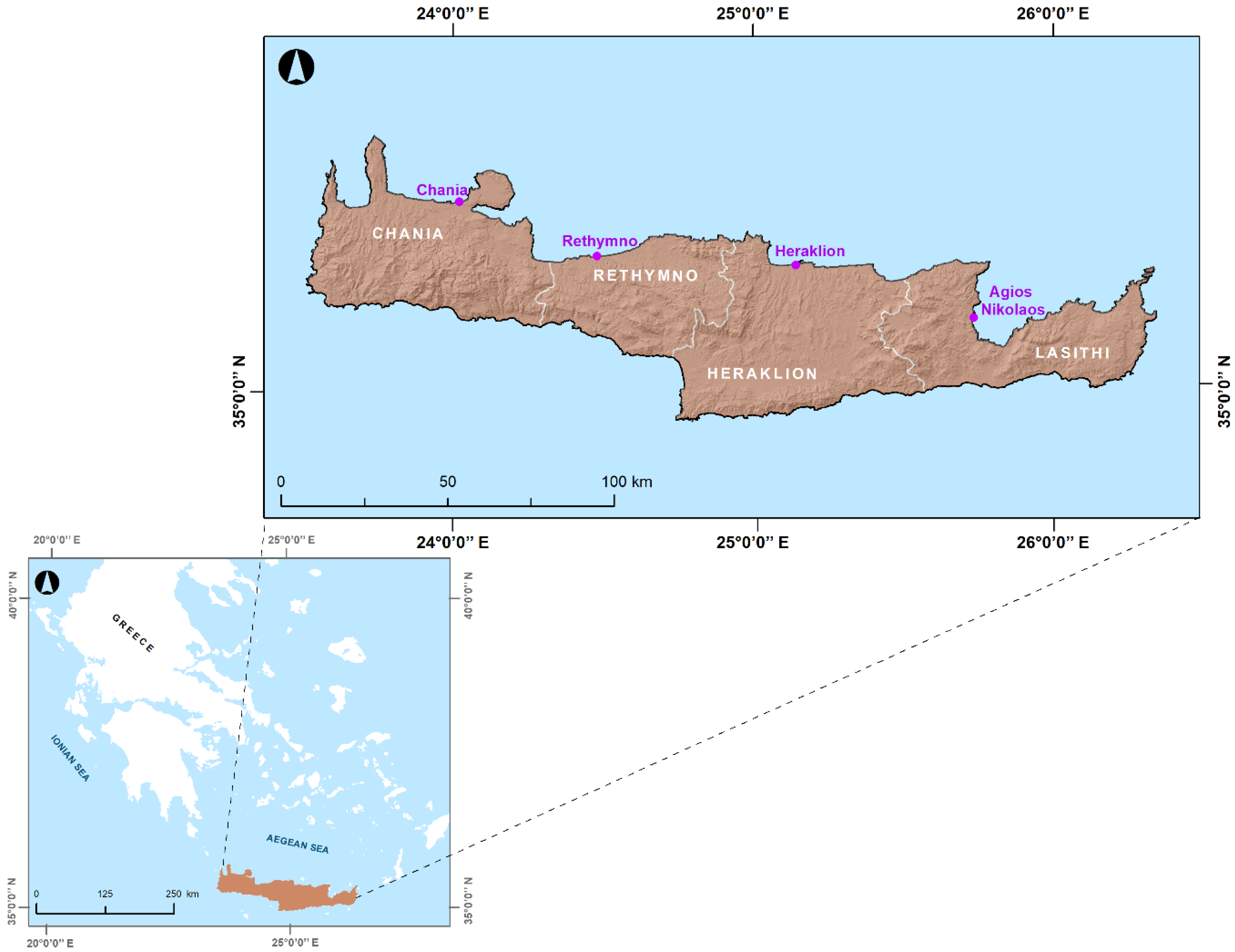
2.1. Study Area

With a total extent of 8257 km2, Crete Island is located in the southern part of Greece (Figure 1), having a distance of 160 km from the Greek mainland and separating the Aegean Sea from the Libyan Sea. The position of the island between the Mediterranean and North African climatic zones, as well as its intense mountainous morphology (with mean elevation at 460 m), have affected its climate. It can be generally characterized as mild with warm and dry summers, and slightly cold and humid winters. The average temperature is 10 °C in the winter season and 30 °C in the summer season, while the mean annual precipitation is about 750 mm, presenting strong spatial and temporal variations [41].
Regarding the geological setting, Crete is composed of pre-Alpine and Alpine carbonate rocks, and Neogene and Quaternary (alluvial) deposits. Particularly, the carbonate geological formations of limestones, marbles and dolomites dominate in the island covering more than 30% of its total area. Permanent crops of olives, vines, and citrus, as well as grasslands, cover most of the island. Heterogeneous croplands or fields mixed with natural vegetation are also detected in a significant part.
The urbanized part of Crete is mainly located in the northern (coastal) zone containing, among others, the capitals of its four administratively determined prefectures: Chania, Rethymno, Heraklion, and Lasithi (from west to east, Figure 1). According to the 2011 census [42], the total population of the island is estimated as 623,065 inhabitants, with the majority of them being concentrated in the four prefecture capitals (Chania, Rethymno, Heraklion, and Agios Nikolaos).

2.2. Data

In order to produce the appropriate factors of RUSLE model, various datasets were collected and analyzed. These datasets contained rainfall, satellite imagery, soil, topographical, and land use/cover data. In particular, a time-series of daily rainfall data covering a period between 1981 and 2019 was obtained from two networks of meteorological stations in Crete: (a) a network of 69 stations operated by the Decentralized Administration of Crete and (b) a network of 21 stations operated by the National Observatory of Athens (NOA). Based on this data, the two years selected for analysis seem to represent two contrasting calendar years in terms of rainfall. The 2019 was the wettest year in the 39-year record (1981–2019) with an average areal rainfall of 1504 mm, while the 2016 was the fourth driest with 646 mm. A time-series of multispectral satellite imagery data acquired from the Sentinel-2 sensor was also used. The choice of acquisition day for each month of the two examined years mainly depended on the need for acquiring images with either none or the least influence by cloud cover limitations. Individual tiles with a spatial resolution of 10 m were extracted from the European Union’s “Copernicus” program as downloadable images through the “Google Earth Engine” [43].
Soil data was derived from two different databases: (a) the “European Soil Database (ESDB) v2.0” provided by the European Soil Data Centre (ESDAC) of Joint Research Centre (JRC) [44] and (b) the harmonized database of derived soil properties for the world (“WISE30sec”) provided by the International Soil Reference and Information Centre (ISRIC) [45]. Shuttle Radar Topographic Mission (SRTM) data at 30 m spatial resolution was exploited to represent the topography of study area as a Digital Elevation Model (DEM). The source of this data was the geoportal of United States Geological Survey (USGS) [46]. Moreover, a set of land use/cover (LUCAS) observation data available by the European statistical authority (Eurostat) [47] was collected. This dataset referred to 2015 and, except for information on land use/cover types appeared in the study area, included some additional information like the slope gradient, presence of support practices, etc.
By using the ArcGIS (v10.4) software package, all the above datasets were organized in GIS thematic layers, of which the source, spatial/temporal resolution and primary format are briefly presented in Table 1.

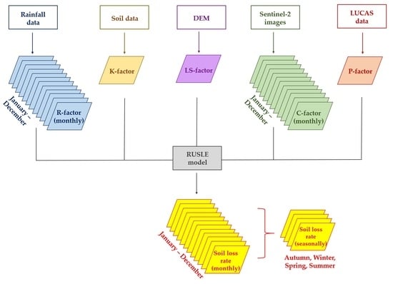
2.3. Revised Universal Soil Loss Equation (RUSLE)

As its name betrays, the Revised Universal Soil Loss Equation (RUSLE) model constitutes the revised version of Universal Soil Loss Equation (USLE) model. It was developed in late 1970s to better estimate the values of the various parameters of USLE [4]. By incorporating improvements in the data analyzed by USLE model, RUSLE enables the estimation of averaged soil loss per unit of area and, thus, the assessment of the spatial distribution of soil erosion within the limits of a given region. Based on the assumption that the detachment of soil and the deposition are controlled by the carrying sediment capacity of flow, RUSLE model integrates a set of five factors describing the main components of water-induced soil erosion. It is based on an empirical expression which can be easily formulated in a GIS framework [48]:
A = R × K × L S × C × P ,
where A is the soil loss (t ha−1), R is the rainfall erosivity factor (MJ mm ha h−1), K is the soil erodibility factor (t ha h ha−1 MJ−1 mm−1), LS is the slope length and steepness factor (dimensionless), C is the cover management factor (dimensionless), and P is the support practice factor (dimensionless). Although Equation (1) is usually used for estimating annual soil loss, it can be modified to a shorter temporal scale (like monthly) by incorporating the dynamic factors of R and C at the corresponding scale.
Rainfall is a prerequisite for any assessment of water-induced soil erosion. Due to its linear relationship with rainfall, the relevant erosivity factor quantifies the effect of the impact of raindrops, and reflects the quantum and rate of runoff that is likely to be associated with the rainfall [9]. It can be determined to estimate either the erosivity for a single storm event or the cumulative erosivity for a series of events within a given time period. R-factor is expressed as a function of the rainfall amount and intensity derived from the analysis of measurement data. The higher the rainfall amount and intensity, the greater the propensity of soil to erosion.
The soil erodibility factor indicates the inherent susceptibility of a specified soil type to detachment and transport by rainfall and runoff. Some soil types are more prone to erosion in terms of physical and chemical properties, such as the texture (contents of silt, sand, clay, and organic carbon), structure, and permeability [49]. These soil properties, typically determined in a laboratory, are analyzed by different empirical formulas to calculate the K-factor [50].
The slope length and steepness factor reflects the effect of topography on soil erosion process. It has been derived from the combination of two individual (sub)factors, the slope length (L) and slope steepness (S). L is considered the distance from the point of origin of overland flow to the point where deposition begins [4]. S is represented by the slope gradient to indicate flat, gentle or steep sloping areas. Increases in L and S lead to higher runoff velocities and, thus, higher soil loss rates. The LS-factor for a given slope can be obtained using measurement data, whereas that in a larger region can be estimated by DEM data [3].
The cover management factor can be defined as the ratio of soil loss from an area with specific vegetation coverage to a continuously fallow area. An increase of vegetation coverage has as result a decrease of soil loss. Owing to the relationship between vegetation coverage and rainfall, the C-factor varies both spatially and temporally. However, it is often parameterized within a land use/cover unit without accounting for its spatio-temporal variability [9,14]. In order to overtake that, an alternative approach has been established including the use of remote sensing-derived vegetation indices to assess the vegetation coverage and its impact on C-factor [18,49]. Several empirical formulas have been developed to relate vegetation indices to the factor estimation [50]. Generally, C-factor ranges from 0 to 1, with values close to 0 being attributed to areas with high vegetation coverage due to limited soil erosion, and those close to 1 to bare lands due to none cover effect on erosion.
Defined as the ratio of soil loss with a specific conservation support practice to the corresponding loss with upslope and downslope cultivation, support practice factor reflects the effects of such practices (e.g., contour farming, tillage, terracing, stone walls, grass margins, etc.) aiming to reduce the eroding power of rainfall-runoff and, thus, reduce the amount of soil loss [51]. The most common approach to produce the P-factor is based on field observations and visual image interpretation. Its values range from 0 to 1, where 0 indicates an area not affected by soil erosion and 1 an area with none conservation support practice.

2.4. Implementation of RUSLE

In order to apply the RUSLE model, the preparation of the component factors was firstly required. For the estimation of R-factor, the regression-based approach originally presented by de Santos Loureiro and de Azevedo [52], and calibrated for the island of Crete by Grillakis et al. [53] was used. The approach estimates monthly rainfall erosivity based on daily rainfall data. It considers the monthly rainfall for days with rain ≥ 10 mm, as well as the number of the days of month with rainfall ≥ 10 mm. The average rainfall erosivity is then estimated according to:
R = 1 n j = 1 n k = 1 m j ( 7.5 · R 10 150 · D 10 ) k , j ,
where R10 is the total rainfall within a month (mm) and only for the days with rainfall ≥ 10 mm (otherwise, set to zero), D10 is the number of days with rainfall ≥ 10 mm, n is the number of days covered by the rainfall data, k is the individual erosive events of each month j, and mj is the total number of erosive events of this month. The R-factor was estimated at point (rainfall station) level. The estimated values were extrapolated to island level by applying ordinary kriging-based interpolation [53] in the ArcGIS environment.
The approach developed by Williams and Renard [54] was applied to estimate the K-factor. It is expressed as follows:
K = 0.2 + 0.3 e ( 0.0256 × S A N × ( 1 S I L 100 ) ) × ( S I L C L A + S I L ) 0.3 × ( 1 0.25 × C C + e ( 3.72 2.95 × C ) ) × ( 1 0.7 S N S N + e ( 5.51 + 22.9 × S A N ) ) ,
where SAN is the sand content (%), SIL is the silt content (%), CLA is the clay content (%), C is the organic carbon content (%), and SN = 1 − (SAN/100). The soil properties included in “WISE30sec” database were linked to the six different soil types of study area from the “ESDB v2.0” within the ArcGIS environment. The K values for the different soil types were then calculated by Equation (3) in order to obtain the spatial distribution of K-factor in the study area.
The LS-factor was created using a hydrology module provided by SAGA GIS (v2.3.2) software package. The module was selected to incorporate the SRTM DEM derivative of slope gradient as S and the approach proposed by Desmet and Govers [55] for L estimation. This approach is defined as:
L = ( A i . j . i n + D 2 ) m + 1 A i , j i n m + 1 D m + 2 × x i , j m × 22.13 m ,
where Ai,j,–in is the contributing area (m2) at the inlet of grid pixel (i,j), D is the grid pixel size (m), xi,j is the summation of the sine and cosine of aspect direction (αi,j) of grid pixel (xi,j = sin αi,j + cos αi,j), and m is a ratio of the rill to interill erosion ranging from 0 to 1.
The C-factor was generated monthly for each time frame (2016 and 2019) by handling the respective Sentinel-2 imagery data. The pre-processing of this data, including atmospheric and radiometric corrections, mosaicking, and cloud cover removal, was initially performed by using JavaScript programming language within “Google Earth Engine”. Based on Earth to Sun distance correction [56] and dark object subtraction [57], the pixel values of 2016 image tiles were converted from original digital numbers into reflectance values. That was not necessary for the 2019 image tiles since they had been already in an atmospherically and radiometrically corrected format. Due to the large size of study area, the corrected image tiles were then mosaicked in order to build a full image for each month of two years covering its total extent. In the monthly images affected by cloud cover limitations, the calculation of a cloud score by using the Red, Green, Blue, Near-infrared (NIR), and Short-wave infrared (SWIR) spectral bands, and the creation of a cloud mask by using the bitmask band (QA60) also took place in terms of pre-processing. The cloud mask was removed and the empty pixels were fulfilled by the values of cloud-free images of directly previous or next months. Afterwards, the Normalized Difference Vegetation Index (NDVI) was calculated in the ArcGIS environment by the following Equation [58]:
NDVI = ρ NIR ρ RED ρ NIR + ρ RED ,
where ρ NIR and ρ RED are the reflectance values at NIR and Red spectral bands, respectively. As an indicator of the energy reflected from the earth’s surface, NDVI has been widely used to represent the various vegetation coverage conditions of several regions [18,49,51]. Its values range between −1 and 1 indicating a lack of vegetation or dense vegetation, respectively. The approach proposed by Van der Knijff et al. [59] was eventually followed to estimate the C-factor as follows:
C = exp [ α ( NDVI β NDVI ) ] ,
where α and β are constants with value 2 and 1, respectively. All the negative C-factor values were set to 0, and the values higher than 1 were set to 1.
Three types of conservation support practices appeared in the island of Crete, such as contour farming, stone walls, and grass margins, were considered for estimating the P-factor of study area. Its estimation in the ArcGIS environment had the form of the product of the (sub)P-factors of these practices [60]:
P = P c f × P s w × P g m ,
where Pcf, Psw, and Pgm are the P-factor values for contour farming, stone walls, and grass margins, respectively. Contour farming includes certain cropland practices, like ploughing or planting, along contours. Since the effectiveness of contour farming in reducing soil erosion depends on the topographic attribute of slope, P-factor values were assigned to the croplands of study area based on the SRTM DEM derivative of slope gradient [61]. It has to be noted that the spatial dataset representing the croplands was derived from the 2018 land cover dataset of the European program “Coordinate of Information on the Environment (CORINE)” [62]. The practices of stone walls and grass margins generally cause a decrease in soil erosion rates by reducing the velocity of overland flow and sediment transport, respectively. The LUCAS observation data as point features could provide information about the locations of stone walls and grass margins in the study area. Based on these points, the density for each of two practices was calculated. This calculation was spatially limited within almost the total of study area (except for “CORINE” artificial surfaces and water bodies) for stone walls and only the “CORINE” agricultural areas (arable land and permanent crops) for grass margins. The P-factor values proposed by Panagos et al. [60] were then assigned to each density result. By using the calculated (sub)P-factors for the three practices in Equation (7), the final P-factor of study area was achieved.
All the factors were organized in GIS raster grids with 30 m spatial resolution (pixel size). Most of them were initially in raster format, while others were converted from vector (polygon or point features) to raster format. By incorporating, every time, in Equation (1), the three static K, LS, and P-factors and each of the monthly R and C-factors, the monthly soil loss maps of Crete Island were produced for 2016 and 2019 (Figure 2, Figure 3, Figure 4 and Figure 5). Furthermore, by averaging the relative monthly soil loss results, similar maps on a seasonal basis were derived (Figure 6). A categorization executed in a manually way according to the presented values was preferred for the total of output maps.

3. Results

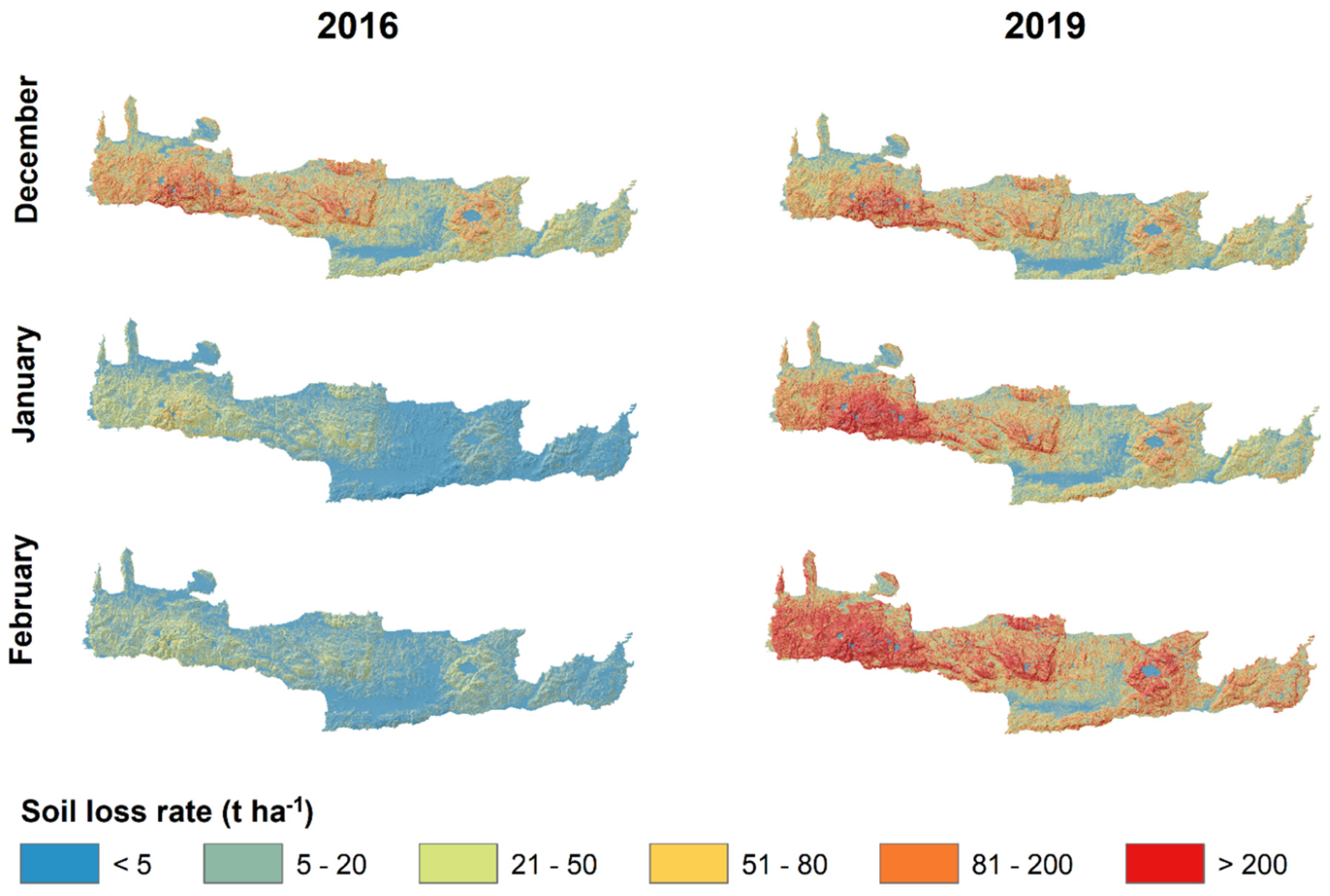
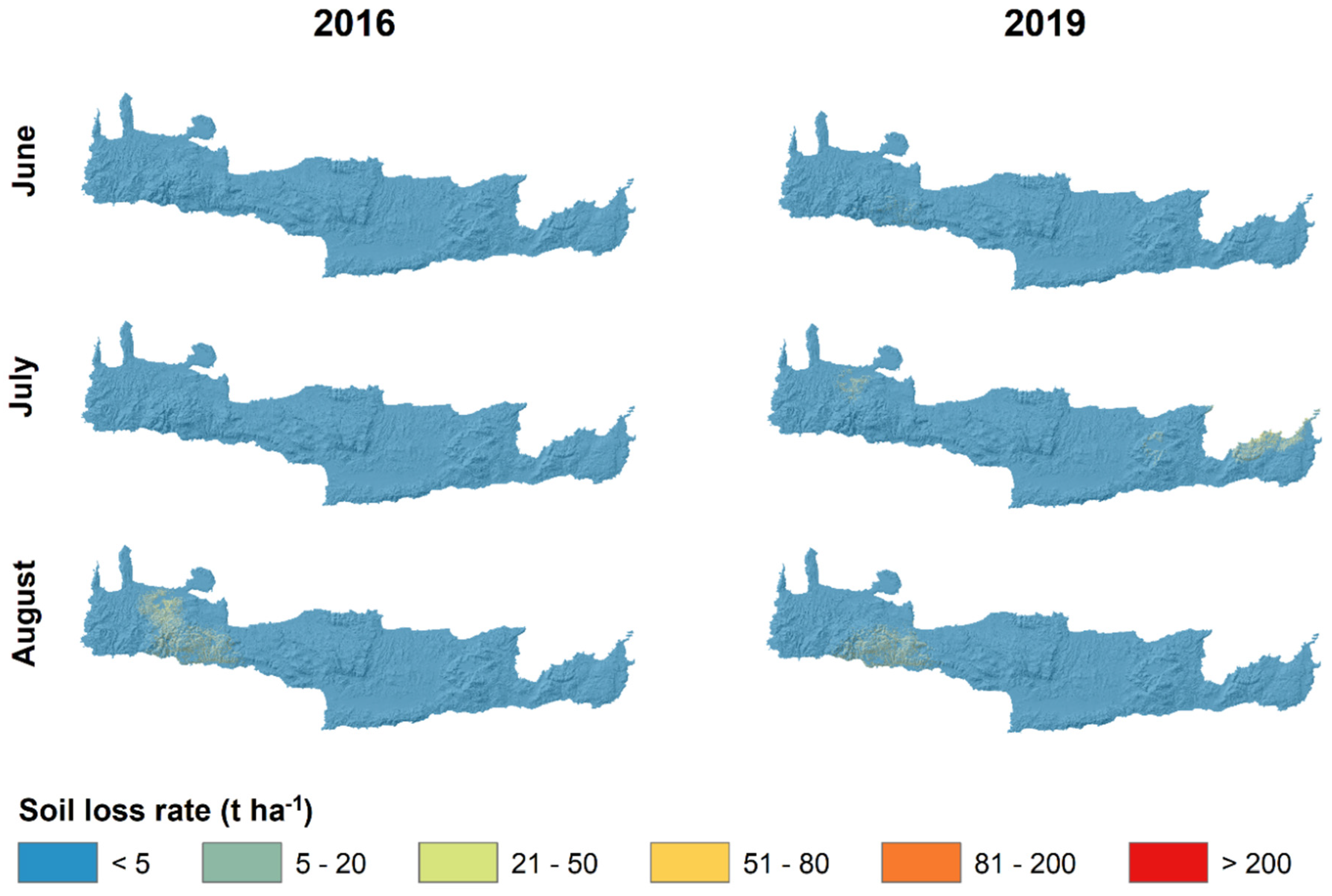
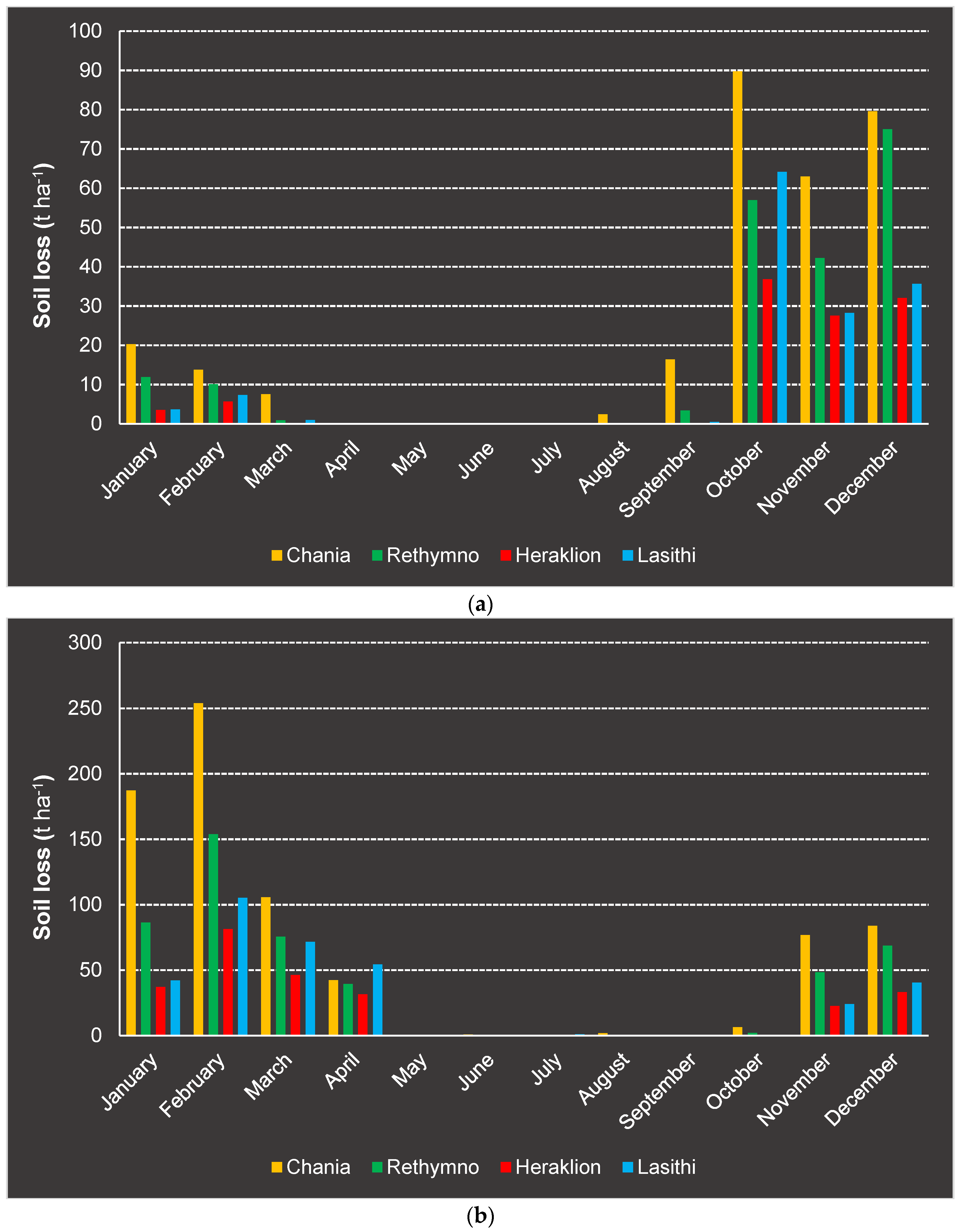
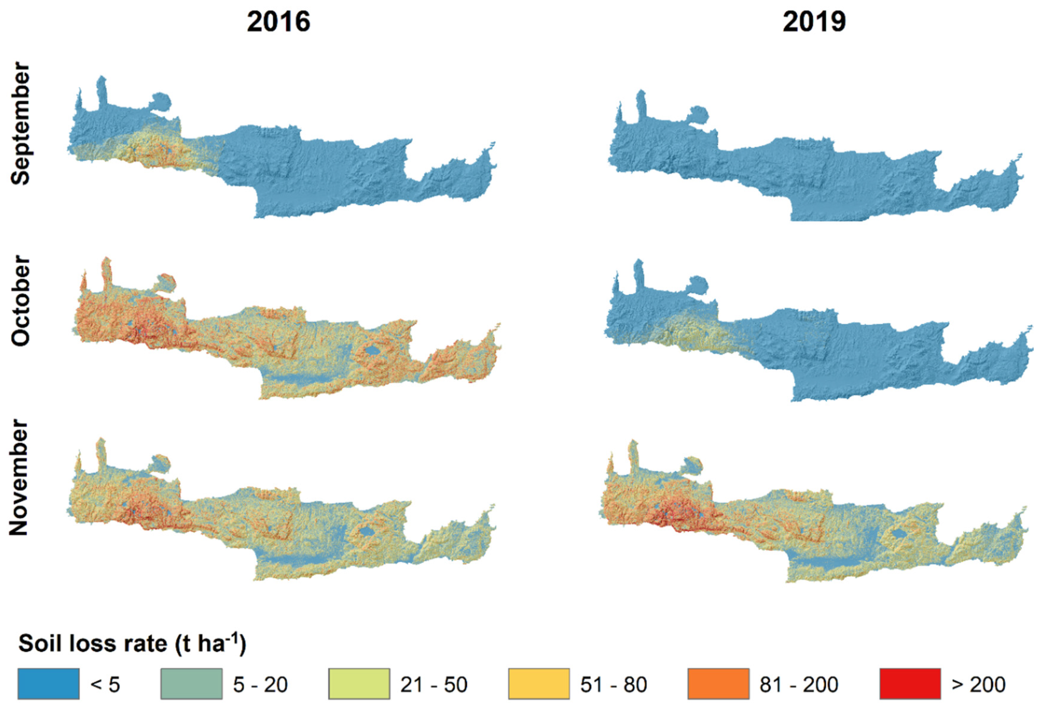
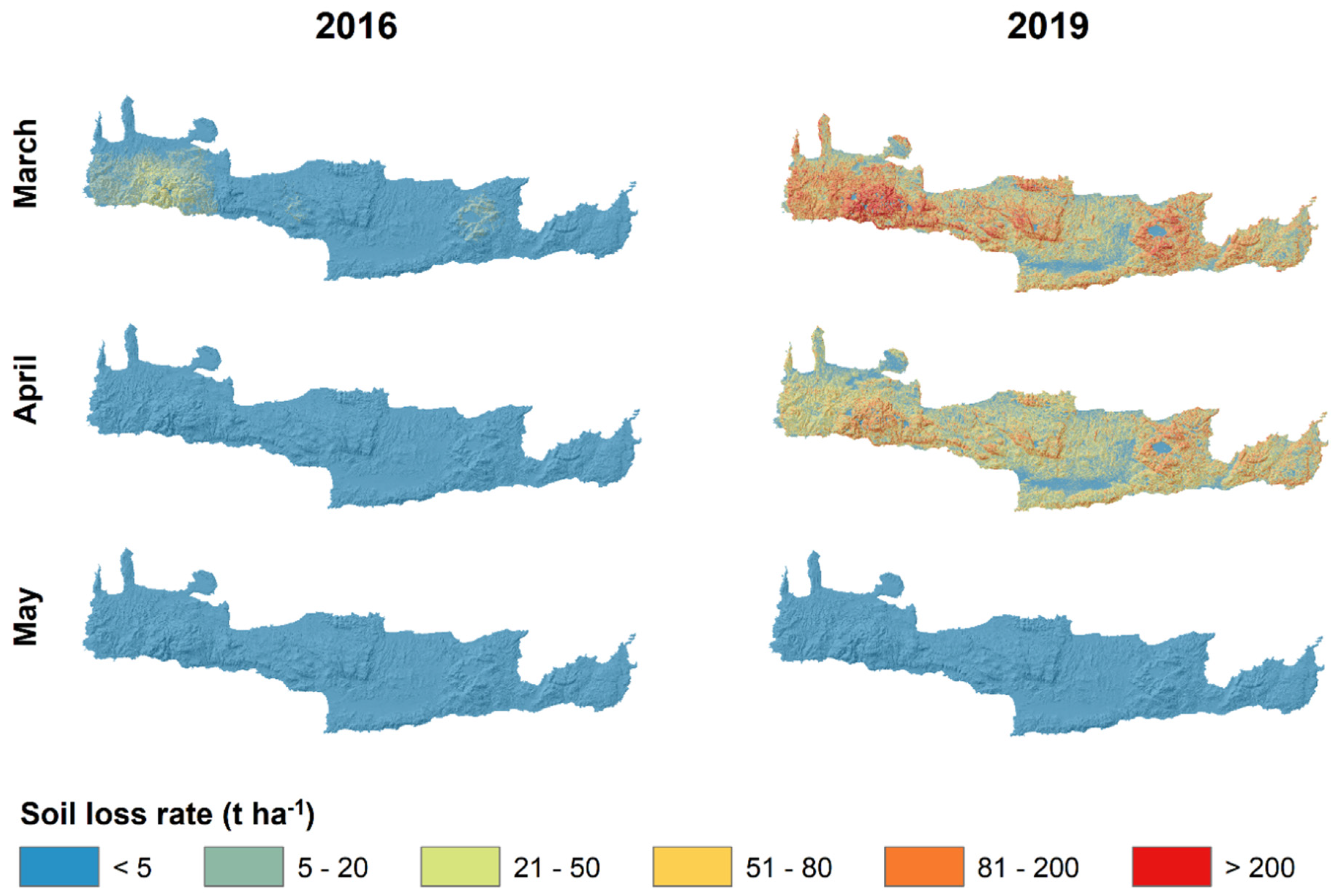
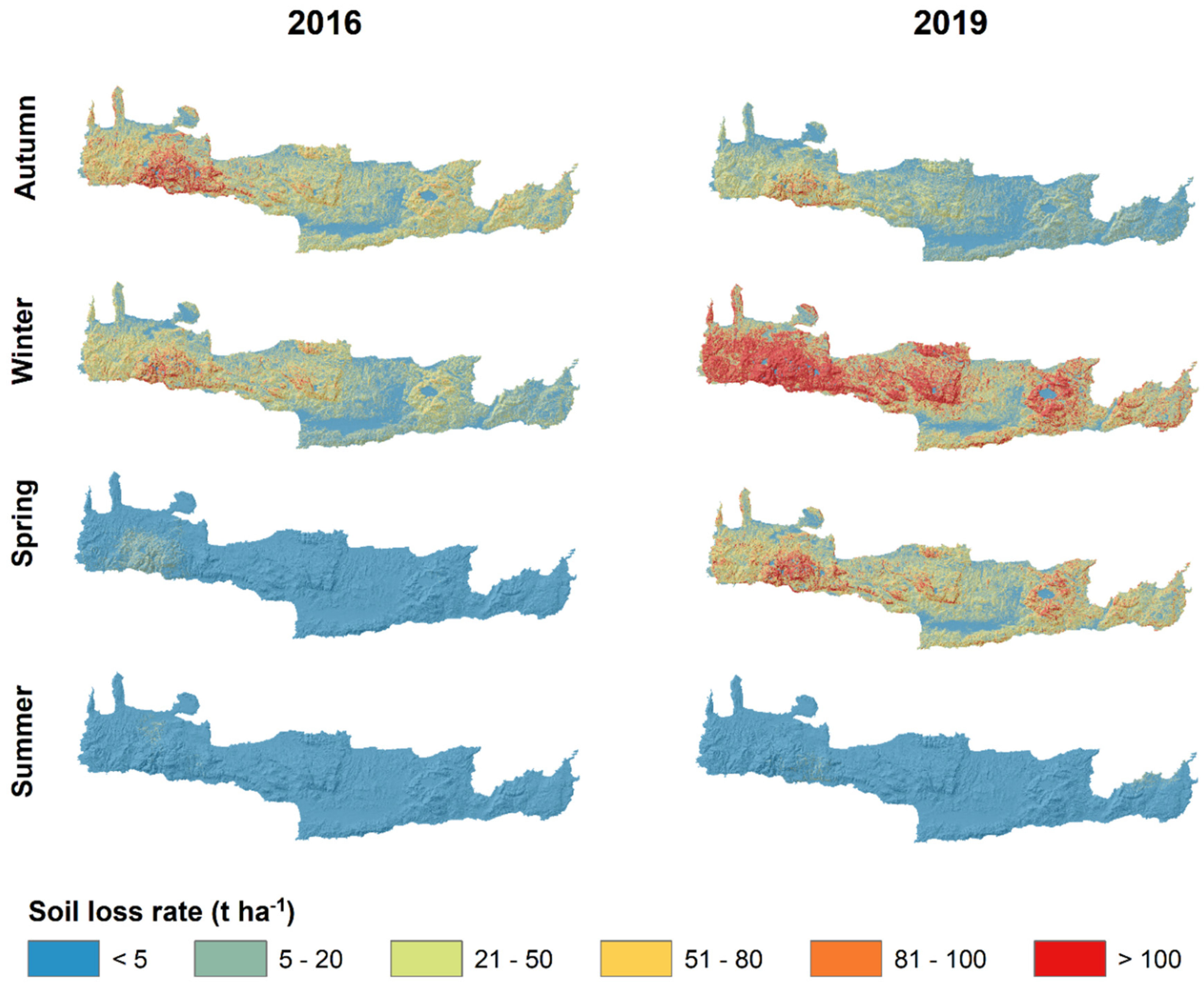
3.1. Monthly and Seasonal Spatial Variations of Soil Loss

Figure 2, Figure 3, Figure 4 and Figure 5 and 6 visualize the spatial distributions of estimated monthly and seasonal, respectively, soil loss rates for Crete Island in 2016 and 2019. In 2016, the period from October to December was identified as the most erosive, with monthly mean soil loss rates greater than 39 t ha−1. Within this period, October was found to have the highest soil loss (mean rate of about 61 t ha−1), followed by December (mean rate of about 53 t ha−1). No influence by water-induced soil erosion was observed at the period from April to July, with monthly mean rates equal to 0 t ha−1. On a seasonal basis, autumn was shown as the most erosive season, with mean soil loss rate equal to about 35 t ha−1. In contrast, summer was the least erosive season, with mean rate equal to 0.22 t ha−1. Both monthly and seasonally, the areas most affected by soil erosion were mainly detected in the west-southern, central, and eastern parts of island.
In 2019, the period from January to March revealed the highest influence by erosion, with monthly mean soil loss rates greater than 70 t ha−1. Among these months, February presented the highest soil loss, with mean rate equal to 146 t ha−1. No influence by erosion (mean rate of 0 t ha−1) was found in September and May. Among seasons, winter was the most erosive (mean rate of about 96 t ha−1), whereas summer was the least erosive (mean rate of 0.25 t ha−1). The areas most affected by soil erosion were mainly observed in the west-southern, central, and eastern parts of island.

3.2. Temporal Variations and Impact of Dynamic Factors on Soil Erosion

The monthly variations of R and C-factors compared with the corresponding soil loss rates were plotted in Figure 7 for evaluating the impact of these variations on soil erosion. Considering their variations in 2016, the low values of R-factor generally presented a downward tendency from January to September. However, the increase from September onwards was notable. In contrast, the tendency of C-factor was slightly upward until September when it started to decrease. In 2019, significantly high R-factor values were observed between the first two months (January and February), followed by an intense decrease until May. From this month to October, the factor was stabilized to values very close or equal to 0. An increase started from October onwards. On the other hand, after fluctuations between January and May, C-factor slightly increased until September when it started to decrease.
In regard to the impact of the two factors and their interactions on estimated soil loss, in 2016, the highly erosive autumn coincided with high rainfall (high R-factor values) and low vegetation coverage (high C-factor values). October emerged to be the most erosive month as a result of the rainfall peak (highest R-factor value) and low vegetation coverage. In spite of low vegetation coverage, the summer showed the lowest soil loss due to not at all or very low rainfall (R-factor values equal or very close to 0). In 2019, the remarkable increase of rainfall (very higher R-factor values) and the slight reduction of dense vegetation coverage (increase in C-factor; however, very low values) led to the indication of winter as the most erosive season. Despite the dense vegetation, February appeared to be the most erosive month due to the observed rainfall peak (highest R-factor value). Moreover, although the vegetation coverage decreased (higher C-factor values), the simultaneously notable decrease of rainfall (very lower R-factor values) revealed the summer as the season with the lowest soil loss.

3.3. Effects of Soil Erosion on Different Spatial Units

In order to quantitatively identify the effects of soil erosion on two different types of spatial units, such as the agricultural areas and administrative prefectures of Crete, the spatio-temporal distribution of monthly soil loss rates per each of two types is illustrated in Figure 8 and Figure 9, respectively. The spatial datasets of agricultural areas were derived from the acquired “CORINE” land cover dataset, and this of prefectures was provided by the National Cadastre and Mapping Agency (NCMA) [63].
Based on the “CORINE” land cover dataset, olive groves, vineyards, fruit trees, and arable land compose the agricultural areas of Crete. Covering the most of agricultural land (87%) and being extended across the entire island, olive groves were found to present the highest monthly soil loss rates in both examined years, especially between October and December in 2016 and between January and March in 2019. At the same temporal periods, olive groves were followed by vineyards, which cover 7% of agricultural land and are mainly concentrated in the central part of island. More or less similar were the rates for the other two agricultural areas, fruit trees (2% of agricultural land, mainly located in the west of island), and arable land (4% of agricultural land, mainly located in the east of island).
In terms of similar to above temporal distribution, among the four prefectures of island, Chania (covering 28% of the total area of island) was shown to be this one with the highest monthly soil loss rates in both 2016 and 2019. With an exception by Lasithi (covering 22% of the total area) in October 2016, Chania was generally followed by Rethymno (covering 18% of the total area). Heraklion prefecture (covering 32% of the total area) was detected to indicate the lowest soil loss over the months of each year.

4. Discussion

Soil erosion is a temporally varying natural process as it is strongly affected by changes in conditioning factors over the time, such as the rainfall and vegetation coverage. In line with that, the present study assessed the intra-annual and inter-annual variations of these factors in determining the monthly and seasonal soil loss variability of Crete Island for two time frames (2016 and 2019). By applying an empirical model like RUSLE, rainfall data at a high temporal resolution and remotely sensed vegetation data time-series constituted the basis for the creation of the appropriate dynamic factors of rainfall erosivity (R) and cover management (C). Due to their static “nature”, the other three factors of soil erodibility (K), slope length and steepness (LS), and support practice (P) were preserved constant.
As a robust, cost-efficient, non-data-demanding and time-consuming erosion model, RUSLE can provide a clear perspective for understanding the interaction of erosion and its influential factors. On this basis, it can identify the erosion changes between months in a simple and systematic way allowing comparisons between them and aggregations over several seasons. Although RUSLE is considered as a leading model in soil erosion assessment, the data availability for generating some of its factors remains a major limitation for maximizing the model accuracy [64]. Furthermore, like in every modeling approach, uncertainties can be implied in the estimation of each incorporated factor.
The outputs of RUSLE model were mapped in order to visualize the spatio-temporal distribution of the estimated soil loss rates in the study area (Figure 2, Figure 3, Figure 4 and Figure 5 and Figure 6). Concerning the spatial distribution, the produced monthly maps revealed that more or less similar areas across the island were affected by high soil loss rates in the most erosive months of the two years. Such large areas mainly located in the south-west, center, and east of island, consist of mountainous bare lands which tend to highly erode under the influence of rainfall. Βased on the seasonal maps, the areas especially located in south-western part of island were found to be the most prone (both in quantity and frequency) to water-induced soil erosion. This finding was found to be in agreement with that by Panagos et al. [40], who resulted to a higher mean erosive value in the west of Crete.
Significant differences were observed in terms of the temporal distribution of high soil loss rates. By an intra-annual perspective (among the months of each year), October in 2016 and February in 2019 were recognized as the most erosive months. Because of the high contribution of these months, and, to a lesser degree, of their temporally closest months (directly previous and next), the relative seasons of autumn in 2016 and winter in 2019 were shown as the most erosive. According to Reference [40], generally 80% of the soil loss is expected in the months between autumn and winter, the rainy period in Crete. Moreover, the indication of summer season and its containing months with the lowest seasonal and monthly mean soil loss rates should be noted for both years. As Baiamonte et al. declared in Reference [18], soil loss generally shows a drop occurring at the summer season, typical of the Mediterranean region. Considering all these intra-annual findings, a temporal “transfer” of high-loss period from autumn to winter could be mentioned by an inter-annual perspective (between the two years).
Regarding the two dynamic RUSLE factors, value-based differences but simultaneously variation-based similarities were detected. Particularly, between 2016 and 2019, two converse tendencies expressed by an increase in the values of R-factor and a decrease in those of C-factor were found (Figure 7). However, each of the two factors presented similar intra-annual variation from one year to the other. R-factor revealed intense fluctuations over the months in both years (especially in 2019), whereas C-factor showed a quite stabilized tendency.
By exploring the impact of their dynamic interactions on soil erosion, the high-loss months (or season) of 2016 were characterized by high R and C-factor values representing high rainfall and low vegetation coverage, respectively. The relative months of 2019 indicated higher soil loss rates as a result of higher R-factor values but lower C-factor values. In other words, from 2016 to 2019, more rainfall combined with more dense vegetation led to higher soil loss. Focusing on that, it could be stated that R-factor seems to be more influential on water-induced soil erosion than C-factor. The matching of values equal to 0 between R-factor and soil loss in specific months of both years (Figure 7) reinforces this finding. In general, the R-factor variability appears to be highly correlated to the monthly rainfall defined, in this case, by the number of the days of month with rainfall ≥ 10 mm. The lower monthly R-factor values, as well as more cases of 0 value, in 2016 evidence the occurrence of lower intensity rainfall, and thus less erosive events, than in 2019. The influence-based “superiority” of R-factor could be mainly attributed to the fact that the C-factor is subjected both to uncertainty in relation to weather and to all related agronomic practices (species choice, seeding date, emergence, crop development, etc.) [18].
Based on the results of monthly soil loss estimations per agricultural land use (Figure 8), particular attention should be given to olive groves since they seemed to have been most affected by water-induced soil erosion in both examined years. The need for planning and taking potential conservation measures for the specific type of agricultural lands could be characterized as imperative. On the other hand, according to the relative results by an administrative perspective, Chania prefecture was found to be most prone in erosion (Figure 9). The increasing amount of rainfall water from east to west as a result of rainfall’s spatial variability [58] could be considered the main natural driving force.

5. Conclusions

The soil erosion occurring in a region may have serious environmental and economic effects. Therefore, the need for understanding this process and identifying the risky periods and areas is crucial. This need is further reinforced due to the emergence of unbalances caused by natural and anthropogenic parameters, such as climate change, intensive agriculture, and wrong land management decisions. Considering that, monthly and seasonal soil loss rates were estimated and mapped for two different years, 2016 and 2019, by using the RUSLE model. The findings revealed that the manipulation of dynamic RUSLE factors (R- and C-factors) at a high temporal resolution provided a variety of spatio-temporal patterns of soil loss which could not be detected at a lower resolution, like the usually applied annual. In particular, the results that would be produced by an annual estimation of soil loss could probably constitute an underestimation of the rates corresponding to risky months (or seasons) and an overestimation of those corresponding to less risky. Furthermore, a more significant impact of the variations of rainfall-related R-factor on soil loss estimations than the vegetation-related C-factor was proved. Based on the output estimations, the riskiest seasons, as well as the spatial units (in terms of agricultural land use and administration division) being most prone to soil erosion, were recognized.
All the above findings could help stakeholders (planners and decision-makers) for elucidating the influential conditions of soil erosion in Crete Island and determining the spatio-temporal variations of soil loss. Under this perspective, the identification of high-loss time periods and areas could constitute the base for evaluating the effectiveness of conservation measures which have been taken in previous years, as well as recognizing the need for potential measures. Some of these measures can be more beneficial if they are taken on the basis of spatial and temporal targeting of specific areas during the riskiest periods of a year. Due to the importance of agricultural lands which predominate the island, the information enabling more targeted interventions for protection of soil resources, mitigation of land degradation risk, and agricultural management is crucial.
Future work could focus on monthly and seasonal soil loss estimations for smaller regions contained in the island (for instance, watersheds) by using data of higher spatial resolution. The differences and similarities between the results derived from the two analysis scales could be then highlighted. Moreover, the comparison of RUSLE with other empirical or different-type models could be another objective of future work.

Author Contributions

Conceptualization, C.P. and D.D.A.; methodology, C.P., D.D.A., M.G.G. and S.M.; formal analysis, C.P., M.G.G. and S.M.; data curation, C.P., M.G.G. and S.M.; writing—original draft preparation, C.P., D.D.A., M.G.G. and S.M.; writing—review and editing; visualization, C.P.; supervision, D.D.A.; project administration, D.D.A.; funding acquisition, D.D.A. All authors have read and agreed to the published version of the manuscript.

Funding

This research is part of a project which has received funding from the Hellenic Foundation for Research and Innovation (HFRI) and the General Secretariat for Research and Technology (GSRT), under grant agreement No 651.

Acknowledgments

The authors acknowledge the National Observatory of Athens and the Decentralized Administration of Crete for providing the observational rainfall data used in the analysis. They also wish to thank the journal’s editor for handling the article, as well as the colleagues who politely considered revising it.

Conflicts of Interest

The authors declare no conflict of interest.

References

  1. Gelagay, H.S.; Minale, A.S. Soil loss estimation using GIS and Remote sensing techniques: A case of Kogawatershed, Northwestern Ethiopia. Int. Soil Water Conserv. Res. 2016, 4, 126–136. [Google Scholar] [CrossRef] [Green Version]
  2. Gianinetto, M.; Aiello, M.; Vezzoli, R.; Polinelli, F.N.; Rulli, M.C.; Chiarelli, D.D.; Bocchiola, D.; Ravazzani, G.; Soncini, A. Future Scenarios of Soil Erosion in the Alps under Climate Change and Land Cover Transformations Simulated with Automatic Machine Learning. Climate 2020, 8, 28. [Google Scholar] [CrossRef] [Green Version]
  3. Fang, G.; Yuan, T.; Zhang, Y.; Wen, X.; Lin, R. Integrated study on soil erosion using RUSLE and GIS in Yangtze River Basin of Jiangsu Province (China). Arab. J. Geosci. 2019, 12, 173. [Google Scholar] [CrossRef]
  4. Wischmeier, W.H.; Smith, D.D. Predicting Rainfall Erosion Losses: A Guide to Conservation Planning; Agriculture Handbook No. 537; US Department of Agriculture Science and Education Administration: Washington, DC, USA, 1978.
  5. Parsons, A.J.; Wainwright, J.; Powell, D.M.; Kaduk, J.; Brazier, R.E. A conceptual model for determining soil erosion by water. Earth Surf. Process. Landf. 2004, 29, 1293–1302. [Google Scholar] [CrossRef]
  6. Choi, K.; Arnhold, S.; Huwe, B.; Reineking, B. Daily Based Morgan–Morgan–Finney (DMMF) Model: A Spatially Distributed Conceptual Soil Erosion Model to Simulate Complex Soil Surface Configurations. Water 2017, 9, 278. [Google Scholar] [CrossRef] [Green Version]
  7. Brooks, E.S.; Dobre, M.; Elliot, W.J.; Wuc, J.Q.; Boll, J. Watershed-scale evaluation of the Water Erosion Prediction Project (WEPP) model in the Lake Tahoe basin. J. Hydrol. 2016, 533, 389–402. [Google Scholar] [CrossRef]
  8. Pandey, A.; Himanshu, S.K.; Mishra, S.K.; Singh, V.P. Physically based soil erosion and sediment yield models revisited. Catena 2016, 147, 595–620. [Google Scholar] [CrossRef]
  9. Sujatha, E.R.; Sridhar, V. Spatial Prediction of Erosion Risk of a Small Mountainous Watershed Using RUSLE: A Case-Study of the Palar Sub-Watershed in Kodaikanal, South India. Water 2018, 10, 1608. [Google Scholar] [CrossRef] [Green Version]
  10. Barmaki, M.; Pazira, E.; Hedayat, N. Investigation of relationships among the environmental factors and water erosion changes using EPM model and GIS. Int. Res. J. Appl. Basic Sci. 2011, 3, 945–949. [Google Scholar]
  11. Bozorgzadeh, E.; Kaman, N. A geographic information system (GIS)-based modified erosion potential method (EPM) model for evaluation of sediment production. J. Geol. Min. Res. 2012, 4, 130–141. [Google Scholar]
  12. Elaloui, A.; Marrakchi, C.; Fekri, A.; Maimouni, S.; Aradi, M. USLE-based assessment of soil erosion by water in the watershed upstream Tessaoute (Central High Atlas, Morocco). Modeling Earth Syst. Environ. 2017, 3, 873–885. [Google Scholar] [CrossRef]
  13. El Jazouli, A.; Barakat, A.; Ghafiri, A.; El Moutaki, S.; Ettaqy, A.; Khellouk, R. Soil erosion modeled with USLE, GIS, and remote sensing: A case study of Ikkour watershed in Middle Atlas (Morocco). Geosci. Lett. 2017, 4, 25. [Google Scholar] [CrossRef] [Green Version]
  14. Koirala, P.; Thakuri, S.; Joshi, S.; Chauhan, R. Estimation of Soil Erosion in Nepal Using a RUSLE Modeling and Geospatial Tool. Geosciences 2019, 9, 147. [Google Scholar] [CrossRef] [Green Version]
  15. Karydas, C.G.; Panagos, P. The G2 erosion model: An algorithm for month-time step assessments. Environ. Res. 2018, 161, 256–267. [Google Scholar] [CrossRef] [PubMed]
  16. Halecki, W.; Kruk, E.; Ryczek, M. Evaluation of water erosion at a mountain catchment in Poland using the G2 model. Catena 2018, 164, 116–124. [Google Scholar] [CrossRef]
  17. Zakerinejad, R.; Maerker, M. An integrated assessment of soil erosion dynamics with special emphasis on gully erosion in the Mazayjan basin, southwestern Iran. Nat. Hazards 2015, 79, S25–S50. [Google Scholar] [CrossRef]
  18. Baiamonte, G.; Minacapilli, M.; Novara, A.; Luciano Gristina, L. Time Scale Effects and Interactions of Rainfall Erosivity and Cover Management Factors on Vineyard Soil Loss Erosion in the Semi-Arid Area of Southern Sicily. Water 2019, 11, 978. [Google Scholar] [CrossRef] [Green Version]
  19. Panagos, P.; Ballabio, C.; Borrelli, P.; Meusburger, K. Spatio-temporal analysis of rainfall erosivity and erosivity density in Greece. Catena 2016, 137, 161–172. [Google Scholar] [CrossRef]
  20. Li, X.; Ye, X. Variability of Rainfall Erosivity and Erosivity Density in the Ganjiang River Catchment, China: Characteristics and Influences of Climate Change. Atmosphere 2018, 9, 48. [Google Scholar] [CrossRef] [Green Version]
  21. Nunes, A.N.; Lourenço, L.; Vieira, A.; Bento-Gonçalves, A. Precipitation and Erosivity in Southern Portugal: Seasonal Variability and Trends (1950–2008). Land Degrad. Dev. 2016, 27, 211–222. [Google Scholar] [CrossRef]
  22. Gu, Z.; Feng, D.; Duan, X.; Gong, K.; Li, Y.; Yue, T. Spatial and Temporal Patterns of Rainfall Erosivity in the Tibetan Plateau. Water 2020, 12, 200. [Google Scholar] [CrossRef] [Green Version]
  23. Yang, X. Deriving RUSLE cover factor from time-series fractional vegetation cover for hillslope erosion modelling in New South Wales. Soil Res. 2014, 52, 253–261. [Google Scholar] [CrossRef]
  24. Alexandridis, T.K.; Sotiropoulou, A.M.; Bilas, G.; Karapetsas, N.; Silleos, N.G. The effects of seasonality in estimating the C-factor of soil erosion studies. Land Degrad. Dev. 2015, 26, 596–603. [Google Scholar] [CrossRef]
  25. Schmidt, S.; Alewell, C.; Meusburger, K. Mapping spatio-temporal dynamics of the cover and management factor (C-factor) for grasslands in Switzerland. Remote Sens. Environ. 2018, 211, 89–104. [Google Scholar] [CrossRef]
  26. Grazhdani, S.; Shumka, S. An approach to mapping soil erosion by water with application to Albania. Desalination 2017, 213, 263–272. [Google Scholar] [CrossRef]
  27. Schmidt, S.; Alewell, C.; Meusburger, K. Monthly RUSLE soil erosion risk of Swiss grasslands. J. Maps 2019, 15, 247–256. [Google Scholar] [CrossRef] [Green Version]
  28. Karydas, C.G.; Panagos, P. Modelling monthly soil losses and sediment yields in Cyprus. Int. J. Digit. Earth 2016, 9, 766–787. [Google Scholar] [CrossRef]
  29. Panagos, P.; Borrelli, P.; Poesen, J.; Ballabio, C.; Lugato, E.; Meusburger, K.; Montanarella, L.; Alewell, C. The new assessment of soil loss by water erosion in Europe. Environ. Sci. Policy 2015, 54, 438–447. [Google Scholar] [CrossRef]
  30. Efthimiou, N. Development and testing of the Revised Morgan-Morgan-Finney (RMMF) soil erosion model under different pedological datasets. Hydrol. Sci. J. 2019, 64, 1095–1116. [Google Scholar] [CrossRef]
  31. Panagopoulos, Y.; Dimitriou, E.; Skoulikidis, N. Vulnerability of a Northeast Mediterranean Island to Soil Loss. Can Grazing ManagementMitigate Erosion? Water 2019, 11, 1491. [Google Scholar] [CrossRef] [Green Version]
  32. Manolis, E.N.; Karetsos, G.K.; Poravou, S.A. Soil erosion risk assessment in a catchment area for ecological monitoring of protected areas using geographic information system. J. Environ. Prot. Ecol. 2019, 20, 146–155. [Google Scholar]
  33. Efthimiou, N.; Psomiadis, E. The Significance of Land Cover Delineation on Soil Erosion Assessment. Environ. Manag. 2018, 62, 383–402. [Google Scholar] [CrossRef] [PubMed]
  34. Stefanidis, S.; Stathis, D. Effect of Climate Change on Soil Erosion in a Mountainous Mediterranean Catchment (Central Pindus, Greece). Water 2018, 10, 1469. [Google Scholar] [CrossRef] [Green Version]
  35. Panagos, P.; Karydas, C.G.; Gitas, I.Z.; Montanarella, L. Monthly soil erosion monitoring based on remotely sensed biophysical parameters: A case study in Strymonas river basin towards a functional pan-European service. Int. J. Digit. Earth 2012, 5, 461–487. [Google Scholar] [CrossRef]
  36. Kouli, M.; Soupios, P.; Vallianatos, F. Soil erosion prediction using the Revised Universal Soil Loss Equation (RUSLE) in a GIS framework, Chania, Northwestern Crete, Greece. Environ. Geol. 2009, 57, 483–497. [Google Scholar] [CrossRef]
  37. Karydas, C.G.; Sekuloska, T.; Silleos, G.N. Quantification and site-specification of the support practice factor when mapping soil erosion risk associated with olive plantations in the Mediterranean island of Crete. Environ. Monit. Assess. 2009, 149, 19–28. [Google Scholar] [CrossRef]
  38. Kourgialas, N.N.; Koubouris, G.C.; Karatzas, G.P.; Metzidakis, I. Assessing water erosion in Mediterranean tree crops using GIS techniques and field measurements: The effect of climate change. Nat. Hazards 2016, 83, S65–S81. [Google Scholar] [CrossRef]
  39. Alexakis, D.D.; Tapoglou, E.; Vozinaki, A.E.K.; Tsanis, I.K. Integrated Use of Satellite Remote Sensing, Artificial Neural Networks, Field Spectroscopy, and GIS in Estimating Crucial Soil Parameters in Terms of Soil Erosion. Remote Sens. 2019, 11, 1106. [Google Scholar] [CrossRef] [Green Version]
  40. Panagos, P.; Karydas, C.; Ballabio, C.; Gitas, I. Seasonal monitoring of soil erosion at regional scale: An application of the G2 model in Crete focusing on agricultural land uses. Int. J. Appl. Earth Obs. Geoinf. 2014, 27, 147–155. [Google Scholar] [CrossRef]
  41. Tapoglou, E.; Vozinaki, A.E.; Tsanis, I. Climate Change Impact on the Frequency of Hydrometeorological Extremes in the Island of Crete. Water 2019, 11, 587. [Google Scholar] [CrossRef] [Green Version]
  42. Hellenic Statistical Authority (ELSTAT). Population and Housing Census: Resident Population. Available online: https://www.statistics.gr/el/statistics/pop (accessed on 29 May 2020).
  43. Google Earth Engine. Available online: https://earthengine.google.com/ (accessed on 14 May 2020).
  44. Panagos, P. The European soil database. Geo Connex. 2006, 5, 32–33. [Google Scholar]
  45. International Soil Reference and Information Centre (ISRIC). WISE Derived Soil Properties on a 30 by 30 Arc-Seconds Global Grid. Available online: https://www.isric.org/projects/world-inventory-soil-emission-potentials-wise (accessed on 12 May 2020).
  46. United States Geological Survey (USGS). EarthExplorer. Available online: https://earthexplorer.usgs.gov/ (accessed on 10 May 2020).
  47. European Statistical Authority (Eurostat). LUCAS Primary Data 2015. Available online: https://ec.europa.eu/eurostat/web/lucas/data/primary-data/2015 (accessed on 17 May 2020).
  48. Renard, K.G.; Foster, G.R.; Weesies, G.A.; McCool, D.K.; Yoder, D.C. Predicting Soil Erosion by Water: A Guide to Conservation Planning with the Revised Universal Soil Loss Equation (RUSLE); Agriculture Handbook; US Department of Agriculture: Washington, DC, USA, 1997; Volume 703, pp. 1–251.
  49. Pal, S.C.; Chakrabortty, R. Simulating the impact of climate change on soil erosion in sub-tropical monsoon dominated watershed based on RUSLE, SCS runoff and MIROC5 climatic model. Adv. Space Res. 2019, 64, 352–377. [Google Scholar] [CrossRef]
  50. Phinzi, K.; Ngetar, N.S. The assessment of water-borne erosion at catchment level using GIS-based RUSLE and remote sensing: A review. Int. Soil Water Conserv. Res. 2019, 7, 27–46. [Google Scholar] [CrossRef]
  51. Maury, S.; Gholkar, M.; Jadhav, A.; Rane, N. Geophysical evaluation of soils and soil loss estimation in a semiarid region of Maharashtra using revised universal soil loss equation (RUSLE) and GIS methods. Environ. Earth Sci. 2019, 78, 144. [Google Scholar] [CrossRef]
  52. de Santos Loureiro, N.; de Azevedo Coutinho, M. A new procedure to estimate the RUSLE EI30 index, based on monthly rainfall data and applied to the Algarve region, Portugal. J. Hydrol. 2001, 250, 12–18. [Google Scholar] [CrossRef]
  53. Grillakis, M.G.; Polykretis, C.; Alexakis, D.D. Past and projected climate change impacts on rainfall erosivity: Advancing our knowledge for the eastern Mediterranean island of Crete. Catena 2020, 193, 104625. [Google Scholar] [CrossRef]
  54. Williams, R.J.; Renard, K.G. EPIC—A new method for assessing erosion’s effect on soil productivity. J. Soil Water Conserv. 1983, 38, 381–383. [Google Scholar]
  55. Desmet, P.J.J.; Govers, G. A GIS procedure for automatically calculating the USLE LS factor on topographically complex landscape units. J. Soil Water Conserv. 1996, 51, 427–433. [Google Scholar]
  56. Martins, V.S.; Barbosa, C.C.F.; De Carvalho, L.A.S.; Jorge, D.S.F.; Lobo, F.D.L.; Novo, E.M.L.M. Assessment of Atmospheric Correction Methods for Sentinel-2 MSI Images Applied to Amazon Floodplain Lakes. Remote Sens. 2017, 9, 322. [Google Scholar] [CrossRef] [Green Version]
  57. Padró, J.-C.; Muñoz, F.-J.; Ávila, L.Á.; Pesquer, L.; Pons, X. Radiometric Correction of Landsat-8 and Sentinel-2A Scenes Using Drone Imagery in Synergy with Field Spectroradiometry. Remote Sens. 2018, 10, 1687. [Google Scholar] [CrossRef] [Green Version]
  58. Polykretis, C.; Grillakis, M.G.; Alexakis, D.D. Exploring the Impact of Various Spectral Indices on Land Cover Change Detection Using Change Vector Analysis: A Case Study of Crete Island, Greece. Remote Sens. 2020, 12, 319. [Google Scholar] [CrossRef] [Green Version]
  59. Van der Knijff, J.M.; Jones, R.J.A.; Montanarella, L. Soil Erosion Risk Assessment in Italy; European Soil Bureau, Joint Research Centre of the European Commission: Ispra, Italy, 1999; p. 52. [Google Scholar]
  60. Panagos, P.; Borrelli, P.; Meusburger, K.; van der Zanden, E.H.; Poesen, J.; Alewell, C. Modelling the effect of support practices (P-factor) on the reduction of soil erosion by water at European Scale. Environ. Sci. Policy 2015, 51, 23–34. [Google Scholar] [CrossRef]
  61. Morgan, R.P.C. Soil Erosion and Conservation, 3rd ed.; Blackwell Publishing: Oxford, UK, 2005; p. 304. [Google Scholar]
  62. Coordinate of Information on the Environment (CORINE) 2018 Land Cover. Available online: https://land.copernicus.eu/pan-european/corine-land-cover/clc2018 (accessed on 18 May 2020).
  63. National Cadastre and Mapping Agency (NCMA). Prefecture Boundaries. Available online: https://geodata.gov.gr/ (accessed on 29 May 2020).
  64. Karamage, F.; Zhang, C.; Liu, T.; Maganda, A.; Isabwe, A. Soil Erosion Risk Assessment in Uganda. Forests 2017, 8, 52. [Google Scholar] [CrossRef]
Figure 1. Location map and study area map presenting the prefectures of Crete Island and their capitals.
Remotesensing 12 02439 g001
Figure 2. Monthly spatial distribution of soil loss rate for Crete Island in 2016 and 2019.
Remotesensing 12 02439 g002
Figure 3. Monthly spatial distribution of soil loss rate for Crete Island in 2016 and 2019.
Remotesensing 12 02439 g003
Figure 4. Monthly spatial distribution of soil loss rate for Crete Island in 2016 and 2019.
Remotesensing 12 02439 g004
Figure 5. Monthly spatial distribution of soil loss rate for Crete Island in 2016 and 2019.
Remotesensing 12 02439 g005
Figure 6. Seasonal spatial distribution of soil loss rate for Crete Island in 2016 and 2019.
Remotesensing 12 02439 g006
Figure 7. Monthly variation of mean soil loss rate in 2016 and 2019 compared to this one of: (a) mean rainfall erosivity (R-factor); (b) mean cover management (C-factor).
Remotesensing 12 02439 g007
Figure 8. Monthly variation of mean soil loss rate per agricultural land use of Crete Island: (a) in 2016; (b) in 2019.
Remotesensing 12 02439 g008
Figure 9. Monthly variation of mean soil loss rate per administrative prefecture of Crete Island: (a) in 2016; (b) in 2019.
Remotesensing 12 02439 g009
Table 1. Summary of input datasets used in Revised Universal Soil Loss Equation (RUSLE) model.
FactorsDatasetsData SourceSpatial/Temporal ScalePrimary Format
Rainfall erosivity (R)Rainfall measurements by stationsNational Observatory of Athens (NOA)Daily, 1981–2019Vector (points)
Decentralized Administration of Crete
Cover management (C)Sentinel-2 images“Copernicus” program10 mRaster (grid)
Soil erodibility (K)Soil types“European Soil Database v2.0” (ESDAC/JRC)1:1,000,000Vector (polygons)
Soil properties“WISE30sec” (ISRIC)30 arc-secondRaster (grid)
Slope length and steepness (LS)SRTM DEMUSGS30 mRaster (grid)
Support practice (P)Land use/cover (LUCAS) observationsEurostat2015Vector (points)

