Using Satellite Thermal-Based Evapotranspiration Time Series for Defining Management Zones and Spatial Association to Local Attributes in a Vineyard

Abstract

A well-planned irrigation management strategy is crucial for successful wine grape production and is highly dependent on accurate assessments of water stress. Precision irrigation practices may benefit from the quantification of within-field spatial variability and temporal patterns of evapotranspiration (ET). A spatiotemporal modeling framework is proposed to delineate the vineyard into homogeneous areas (i.e., management zones) according to their ET patterns. The dataset for this study relied on ET retrievals from multiple satellite platforms, generating estimates at high spatial (30 m) and temporal (daily) resolutions for a Vitis vinifera Pinot noir vineyard in the Central Valley of California during the growing seasons of 2015-2018. Time-series decomposition was used to deconstruct the time series of each pixel into three components: long-term trend, seasonality, and remainder, which indicates daily fluctuations. For each time-series component, a time-series clustering (TSC) algorithm was applied to partition the time series of all pixels into homogeneous groups and generate TSC maps. The TSC maps were compared for spatial similarities using the V-measure statistic. A random forest (RF) classification algorithm was used for each TSC map against six environmental variables (elevation, slope, northness, lithology, topographic wetness index, and soil type) to check for spatial association between ET-TSC maps and the local characteristics in the vineyard. Finally, the TSC maps were used as independent variables against yield (ton ha-1) using analysis of variance (ANOVA) to assess whether the TSC maps explained yield variability. The trend and seasonality TSC maps had a moderate spatial association (V = 0.49), while the remainder showed dissimilar spatial patterns to seasonality and trend. The RF model showed high error matrix-based prediction accuracy levels ranging between 86% and 90%. For the trend and seasonality models, the most important predictor was soil type, followed by elevation, while the remainder TSC was strongly linked with northness spatial variability. The yield levels corresponding to the two clusters in all TSC were significantly different. These findings enabled spatial quantification of ET time series at different temporal scales that may benefit within-season decision-making regarding the amounts, timing, intervals, and location of irrigation. The proposed framework may be applicable to other cases in both agricultural systems and environmental modeling.

1. Introduction

Precision irrigation for agricultural activities is a key factor for managing yield and quality, minimizing the use of water resources, and maximizing crop production. Irrigation practices generally relate to the timing, amounts, and spatial distribution of water input [1]. Therefore, both spatial and temporal information about various field characteristics is required to enable precision irrigation applications. Extensive research has been published regarding location and allocation of water input in the field, also involving the optimal timing of irrigation for specific types of crops [2,3,4]. Accurately quantifying the amount, timing, and location of irrigation depends both on the method of irrigation [5,6] and on accurate information regarding meteorology, terrain, plant, and soil conditions [7,8]. Site-specific management is an important factor in precision agriculture. The leading approach for differential management of the field is based on the delineation of the agricultural plot to management zones (MZs), which are homogenous sub-field areas based on within-field spatial variability [9]. There is an ongoing effort in the scientific community to develop and improve accurate and representative methods for defining MZs for specific purposes such as irrigation, fertilization, and pest control [10,11,12]. In vineyards, specifically for wine production, the amount of water provided to the grapevines is highly associated with vegetative growth, yield, and attributes related to quality traits, such as sugar content, acidity, and pigment content [1]. Water stress levels in vines are often highly variable across the vineyard [13,14]. Therefore, differential irrigation treatments are required, based on defined MZs, to comply with dissimilar water demands by the vines according to the target yield quality and quantity specified by the grower [15].

Evapotranspiration (ET) is defined as water loss to the atmosphere by evaporation from the soil surface and transpiration from the canopy cover. ET is a difficult water balance component to measure and estimate since it is affected by multiple atmospheric variables (e.g., wind speed, relative humidity, temperature and solar radiation) [16] as well as plant physiology [17,18]. The ability to quantify ET values in the field is highly valuable for determining the water stress of the crops and planning the amounts and timing of irrigation at different timesteps during the growing season [19,20]. Over the past two decades, many techniques for acquiring information regarding ET levels have been proposed and successfully applied [21,22,23]. However, these approaches lack the ability to provide routine spatial information about sub-field heterogeneity in plant conditions and water use/stress. In response, several satellite remote sensing-based algorithms have been developed and have demonstrated the utility of such an approach when attempting to quantify within-field heterogeneity in crop water use [24,25,26,27]. These algorithms include the Surface Energy Balance Algorithm for Land (SEBAL; [28]), Mapping Evapotranspiration with Internalized Calibration (METRIC; [26]), the Surface Energy Balance System (SEBS; [25]), and the Two-Source Energy Balance model (TSEB; [29]). The commonality between these approaches is that they predominantly rely on thermal infrared (TIR) imagery to approximate land surface temperature (LST) characteristics and then estimate ET as the residual component of the energy balance equation. These approaches have been used extensively and have been validated over many landcover types. A subset of ET mapping algorithms, including the Atmosphere-Land Exchange Inverse (ALEXI) model [27,30] and associated flux disaggregation technique (DisALEXI) [31,32] have been applied over vineyards, showing promising results [33,34,35,36,37].

The paired ALEXI/DisALEXI approach is predicated on the retrieval of LST from TIR imagery, which has been shown to be particularly useful in monitoring ET and plant stress due to its sensitivity to variations in soil moisture availability [38]. The approach calculates ET on both high-spatial/low-temporal (e.g., Landsat) and moderate-spatial/high-temporal (e.g., the Moderate Resolution Imaging Spectroradiometer; MODIS) resolution grids before being merged using the Spatial and Temporal Adaptive Reflectance Fusion Model (STARFM) [39]. Combining data from multiple sensors via data fusion provides daily ET estimates at field scale resolution, allowing for the quantification of both spatial and temporal dynamics in the field. Studies were conducted over two Pinot noir vineyards located near Lodi, CA, as a part of the Atmospheric Profile and Evapotranspiration eXperiment (GRAPEX; [35]). Since the inception of GRAPEX in 2013, the application of ALEXI/DisALEXI over vineyards has expanded to sites in Northern California (Sonoma County) and the southern Central Valley of California (Fresno County) [40].

Spatiotemporal dynamics in agricultural fields have been studied for decades [41,42,43]. The outcomes of these analyses were commonly a series of maps or descriptive statistics highlighting spatial variability in each time step [44]. In some cases, with a minimal number of time steps, this method is sufficient to emphasize the differences. However, in other studies where the timeframe includes many images/maps, an additional analysis was usually conducted to emphasize the temporal variation in space [45,46]. Quantification of ET over space is commonly represented on a daily scale, thus involving hundreds of images. Research in the past years has focused on mapping field characteristics, such as canopy cover and ET, at the field/landscape scale for each time step [37,47]. Alternatively, defining MZs based on within-field spatial variability provides information regarding the spatial heterogeneity in the field [48,49]. However, this approach does not provide any information regarding the temporal variation. Not many studies provided a framework to analyze the effect of spatially varying attributes on the temporal pattern [50]. For irrigation purposes, none of the mentioned approaches contributed an indication regarding the crop water status and the amount of input to be implemented in each MZ. Using daily ET assessments at the vineyard scale not only enables one to determine a spatial separation of the field into MZs based on ET temporal variations, but also to provide a complete status of the typical ET temporal dynamic of each MZ for irrigation purposes.

While time-series clustering (TSC) using remote-sensing data has been proposed in the past [51], very few studies have used this technique, mostly for land-cover monitoring [52]. To the best of our knowledge, no previous efforts have been made to use TSC for delineating MZs in agricultural fields, or to characterize the spatial attributes underlying the TSC spatial patterns.

The main objective of this study was to characterize the spatial and temporal patterns of ET within a vineyard. The specific objectives were: (1) to use time-series decomposition of ET into three components, including trend, seasonality, and remainders; (2) to cluster each of the three ET components into MZs using time-series clustering; (3) To quantify the impact of spatial field attributes on the spatial patterns of ET at different time scales (components); (4) to analyze the spatial effect of ET for each time component on grapevine yield.

2. Materials and Methods

2.1. Study Area

The vineyard under study is located in the Central Valley of California, near the city of Lodi (Figure 1), and is part of the USDA-ARS GRAPEX [35]. This area is characterized by a Mediterranean climate, with warm, dry summers and wet winters, with occasional spring rainfall events. The vineyard was planted in 2009 with Pinot noir vines and installed with drip irrigation. It has an area of 35 ha with an East-West row orientation and spacing of 1.5 m between vines and 3.3 m between rows [36]. Budbreak in the vines typically occurs at mid-March and harvest in late August/early September. The leaves then reach senescence and start to defoliate towards the dormancy period in the winter. Two vernal pools are located within the vineyard (Figure 1) and were masked out since they do not represent the temporal structure of grapevine ET. In addition, the pixels at the borders of the vineyard were masked out as well, due to the potential impact on the border vines from external sources [53] and mixed-pixel effects. This was done by removing one column from the eastern and western parts of the vineyard, as well as the northern and southern rows. The vineyard is equipped with a meteorological/flux tower located approximately half-way north-south along the eastern edge of the field. Precipitation amounts were measured using a tipping bucket rain gauge (TE525, Texas Electronics, Dallas, Texas).

2.2. Data Collection–ET Images, Environmental Attributes, and Yield

2.2.1. ET Images

This study applied the ALEXI surface energy balance model [27] and the associated disaggregation algorithm (DisALEXI) [31,32] in conjunction with STARFM [39] to derive daily images of ET over the vineyard of interest. ALEXI relates changes in LST, derived from geostationary satellites, to latent heat flux and surface moisture availability to estimate daily 4 km ET fluxes. These coarse resolution ET fluxes are spatially downscaled (DisALEXI) using higher resolution LST information from MODIS (1 km) and Landsat (30 m). They are then combined using STARFM to produce daily 30 m ET maps.

ALEXI is based on the TSEB model [29], which is unique in that it partitions radiometric temperature, T_RAD, into soil and canopy temperatures (Ts and T_c, respectively), given the vegetation cover fraction (f) at radiometer view angle (θ):

$$T_{RAD}\left(\theta \right)={\left[f\left(\theta \right)T_c^4+\left[1-f\left(\theta \right)\right]T{s}^4\right]}^{\frac{1}{4}}$$

(1)

These component temperatures are then used to solve the energy balance equation for a mixed scene by combining soil and canopy contributions:

$$\left(R{n}_s+R{n}_c\right)-G=\left(H_s+H_c\right)+\left(\lambda E_s+\lambda E_c\right)$$

(2)

where Rn is net radiation (W/m²), H is sensible heat flux (W/m²), G is soil heat flux (W/m²), and λE is the latent heat flux (W/m²). As in Equation (1), subscripts “s” and “c” refer to soil and canopy components, respectively. TSEB is applied twice during the morning, roughly 1 h after sunrise and again 1 h before local noon, using radiometric temperature acquired from the Geostationary Operational Environmental Satellites (GOES) platform. Energy closure during this time interval is provided by a simple slab model of atmospheric boundary layer development [54] which internally simulates land-atmosphere feedback on near-surface air temperature. As a result of using a time-differential approach, the flux errors due to absolute sensor calibration, atmospheric corrections, and emissivity corrections are minimized [55].

ALEXI produces fluxes at 4 km spatial resolution, which is too coarse for field-scale applications. In order to provide field-scale flux estimates, the associated spatial disaggregation technique known as DisALEXI [32] was implemented. DisALEXI utilizes higher resolution TIR imagery (MODIS, Landsat, airborne sensors) to spatially disaggregate the coarser-resolution ALEXI flux estimates. This is done by running TSEB over each ALEXI pixel within a user-defined modeling domain, using TIR information at time of overpass from a satellite of interest (MODIS, Landsat, airborne sensor) as input. The air temperature boundary condition (set at a nominal blending height of 50m) for an ALEXI pixel is iteratively adjusted until the DisALEXI ET fluxes, spatially averaged over the ALEXI pixel, converge. This ensures consistency between the ALEXI and DisALEXI fields.

DisALEXI ET fluxes are upscaled from overpass time (instantaneous) to daily total estimates using the ratio of instantaneous to daily insolation:

$$E{T}_{day}=\frac{\lambda E_{t2}}{R_{s_{t2}}}\left(\frac{R_{s24}}{\lambda \rho w}\right)$$

(3)

where λE_t2 is the latent heat at t2, Rs_t2 is the insolation rate at t2, R_s24 is the time-integrated daily insolation rate, λ is the latent heat of vaporization, and $\rho w$ is the density of water. The reader is referred to [39,56,57] for detailed descriptions of the ET modeling process. Applications over the current vineyard (Lodi) are described by [33,36,40].

Previous studies report good agreement between ALEXI/DisALEXI-derived daily ET and eddy covariance flux tower measurements, regardless of vineyard location. Specifically, Semmens et al. [33] reported root mean square error (RMSE) of under 1 mm day⁻¹ at the Lodi site for the 2013 growing season. Knipper et al. [36] reported slightly lower RMSE values (0.8 mm day⁻¹) at the same site when extending the analysis through 2016. When compared over multiple vineyards characteristic of having different grape varieties, trellis designs, canopy structure, irrigation management and climate conditions, the ALEXI/DisALEXI model produced daily ET estimates with good fidelity (RMSE values of 0.88 mm day⁻¹ on average between sites) [40].

ET images from four consecutive growing seasons, between 2015 and 2018, were used in this study. The growing season of grapevines is typically from early spring until mid-fall, while the vines are covered with transpiring leaves. Therefore, a subset was taken from the four-year dataset, from March 1 to October 31 (days of year (DOY) 60-304) of every year (Figure 2). The selected images included 71 Landsat scenes and 980 MODIS scenes. Following the STARFM fusion process, there were 980 high resolution (30m) ET images, with 245 images per growing season. Few images had missing ET values due to weather conditions that did not allow for clear MODIS images, and the missing data for each pixel was interpolated using a temporal moving average with a window of 4 days. This procedure was performed using the “imputeTS” package in R [58].

2.2.2. Environmental Attributes

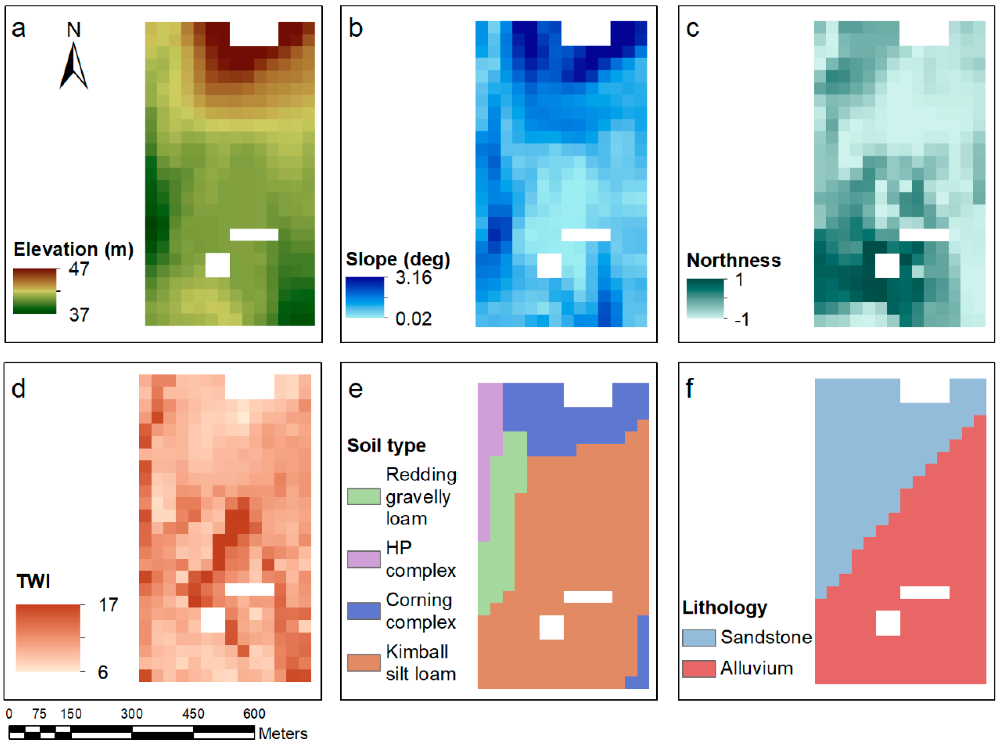
Six different spatial environmental attributes were acquired to check for their influence on the spatial pattern of the ET time series in the vineyard. These covariates included the following (Figure 3):

• Digital elevation model (DEM): Represents shifts in elevation (m) at a 30 m spatial resolution. The variability in elevation is known to affect plant conditions [59] and ET across space [60]. Within the study area, the elevation ranges between 37 and 47 m above sea level, with a median of 40.5 m above sea level.
• Slope: Derived from the DEM, with identical spatial resolution and coordinate system. It was computed as the highest difference between a certain pixel and its 8 neighboring cells [61] and was applied using the “raster” package in R [62]. The slope is known to have an impact on soil water content [63], thereby affecting the water availability to the plant [64] and its water consumption levels. The slope in the vineyard is considered moderate, ranging between 0 and 3.16°, with a median of 0.75°.
• Northness: Derived from the DEM with an inherent 30 m spatial resolution. Aspect was computed as the gradient vector at each pixel location according to the direction between neighboring pixels, such that the North is defined as 0° and south as 180°. The aspect was derived using the R package “raster” [62]. To avoid using a circular variable in a regression model, aspect was transformed to northness, which is the cosine of aspect [65,66]. Aspect is known to affect the levels of exposure to solar radiation by the plants, thereby influencing plant water conditions, with significant effects between North- and South-facing slopes [67]. The west side of the vineyard is mostly facing West, North, and North-West, while the East side of the vineyard is mostly facing East and South-East.
• Topographic wetness index (TWI): Represents soil moisture conditions and quantifies the distribution of accumulated area across downslope pixels. It was calculated by Equation (4) using the “dynatopmodel” package in R [68]:

  TWI = ln(A/tanβ)

  (4)

  where A stands for the upstream contributing area (m2) for each pixel and β is the local slope in the steepest downhill direction (degrees). TWI is used to assess the soil moisture and its effects on plant conditions [69]. TWI levels ranged between 6 and 17 with a median of 9.
• Soil types: The soil type map represents different soil groups within the vineyard, represented as polygons, as classified in the Gridded Soil Survey Geographic (gSSURGO) Database. The soil types layer was spatially overlaid over the raster dataset to retrieve the indexes of the soil classes for each pixel, using R package “sp” [70]. Soil texture and structure are among the main attributes affecting soil moisture levels and soil water extraction patterns [71] due to variations in soil depth, permeability levels, micronutrients, and more [72,73]. In turn, these soil properties affect water availability to the plant and ET levels [74]. There are four soil type classes within the vineyard domain (SSHCP, 2018), including the following:
  Redding gravelly loam: Associated with the Laguna Formation, which is associated with high terrace landform, and composed of interbedded alluvial gravel, sand, and silt. This soil series developed on older, higher alluvial terrace landforms, is a well-drained, gravelly loam mineral soil that is moderately deep and formed in gravelly valley fill [75]. The water holding capacity in low and permeability is very slow, reaching 50-100 cm [72].
  Hadselvill-Pentz complex: Consists of very shallow loamy, moderately well-drained intermound soils. This soil series is associated with the Mehrten Formation, which consists of eroded, volcanic mudflow fans. It has organic matter content of 1%-2% and is very shallow [75], with moderately rapid permeability, reaching 10-50 cm. Water holding capacity is very low [72].
  Corning complex: Formed of gravelly loam from the Laguna Formation and gravels on high terraces. They have microrelief composed of a mound-intermound structure on smooth terrace side slopes. These are very deep soils, well-drained with a gravelly fine sandy loam surface layer [75]. Permeability in this soil series is very low. After rainfall events/irrigation, the soil is saturated for a short time [72].
  Kimball silt loam: The Kimball series consists of well-drained loams. They were formed on older terraces in alluvium derived from sedimentary rocks [76]. Its subsoil permeability reaches 150+ cm, with a moderate water holding capacity and slow runoff [72].
• Lithology: The lithology map represents the spatial distribution of rock formation within the vineyard, represented as polygons, and the same technique was used to extract the classes representing each pixel as for the soil types layer. The lithology may have an effect on water availability to the plant [77] and its ability to consume water. This covariate included two classes – Sandstone on the northwest part of the plot and alluvium in the southeast part of the vineyard.

The DEM [78], soil types [79], and lithology [80] covariates were acquired from the Geospatial Data Gateway site (https://gdg.sc.egov.usda.gov/) of the United States Department of Agriculture (USDA).

2.2.3. Yield

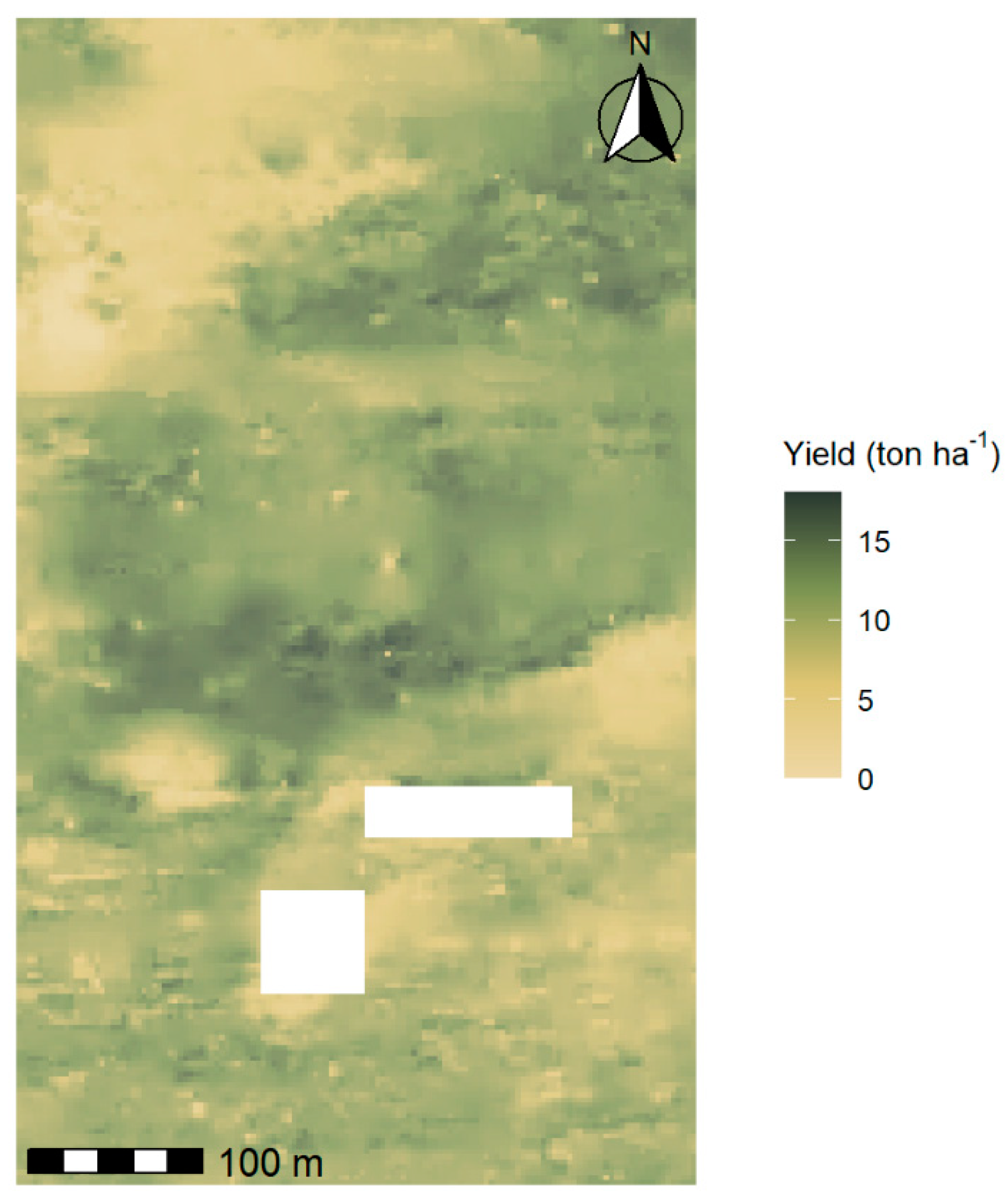
A yield map was also used for analyzing the association between ET spatial pattern and yield levels [21]. The yield map (Figure 4) was provided by E&J Gallo Winery using Advanced Technology Viticulture (ATV, Joslin, Australia) yield monitoring systems that were applied in the vineyard during the harvest in August 22, 2016. Post-harvest analysis converts mass flow units into tons per hectare, eliminates outliers (yield data greater than three standard deviations from the mean), and normalizes across harvesters. The yield map was interpolated to a 3-m grid using Vesper Spatial Prediction Software for Precision Agriculture [81]. The Northern-most grapevine rows are masked out due to spurious detected artifacts.

2.3. Time-Series Decomposition and Clustering of Each Component

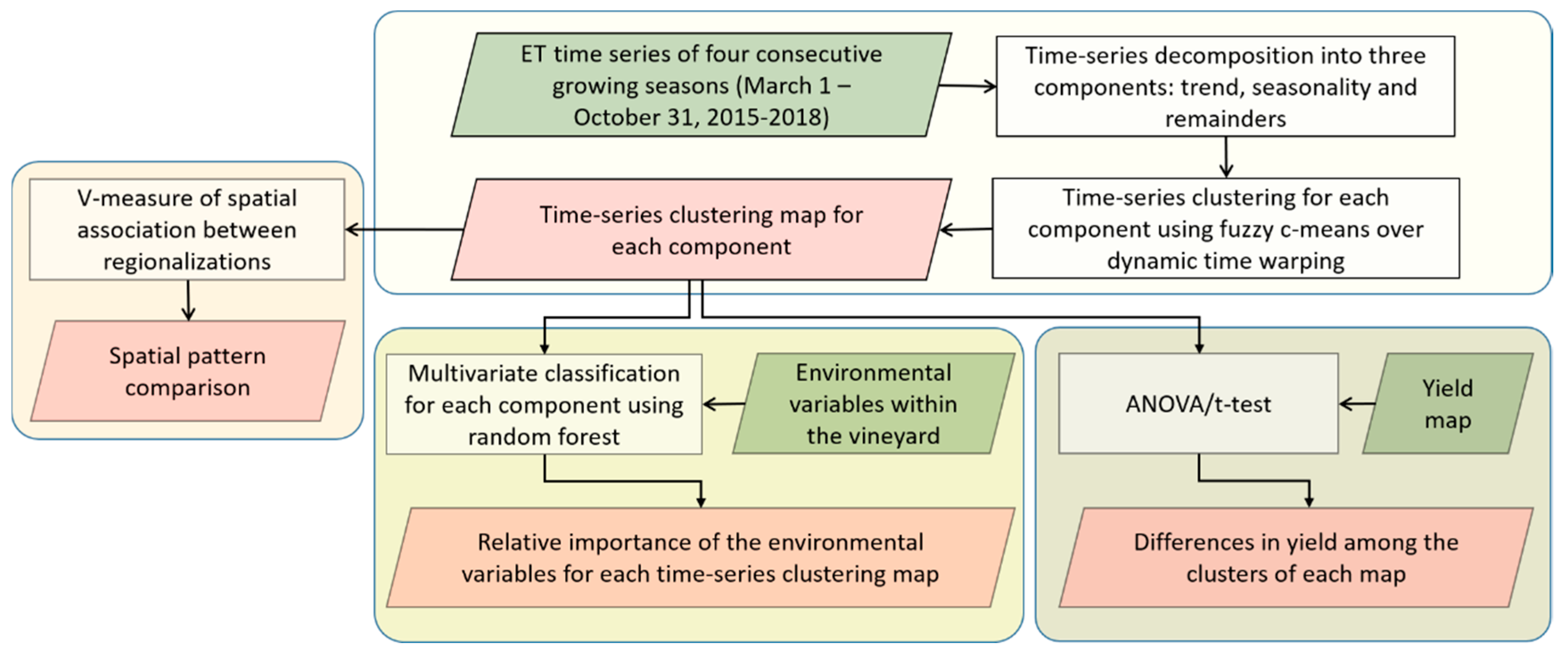
The ET time series of each pixel was decomposed into three different time components. In order to comply with specific objective 2, a TSC procedure was applied to each of the components. In general, TSC is a process during which time series data is partitioned into homogeneous groups based on the similarities of the time series values and temporally varying patterns [82]. The data composing a time series is dynamic, its values change as a function of time and clustering of time series may reveal patterns and changes [82]. TSC relied on four elements:

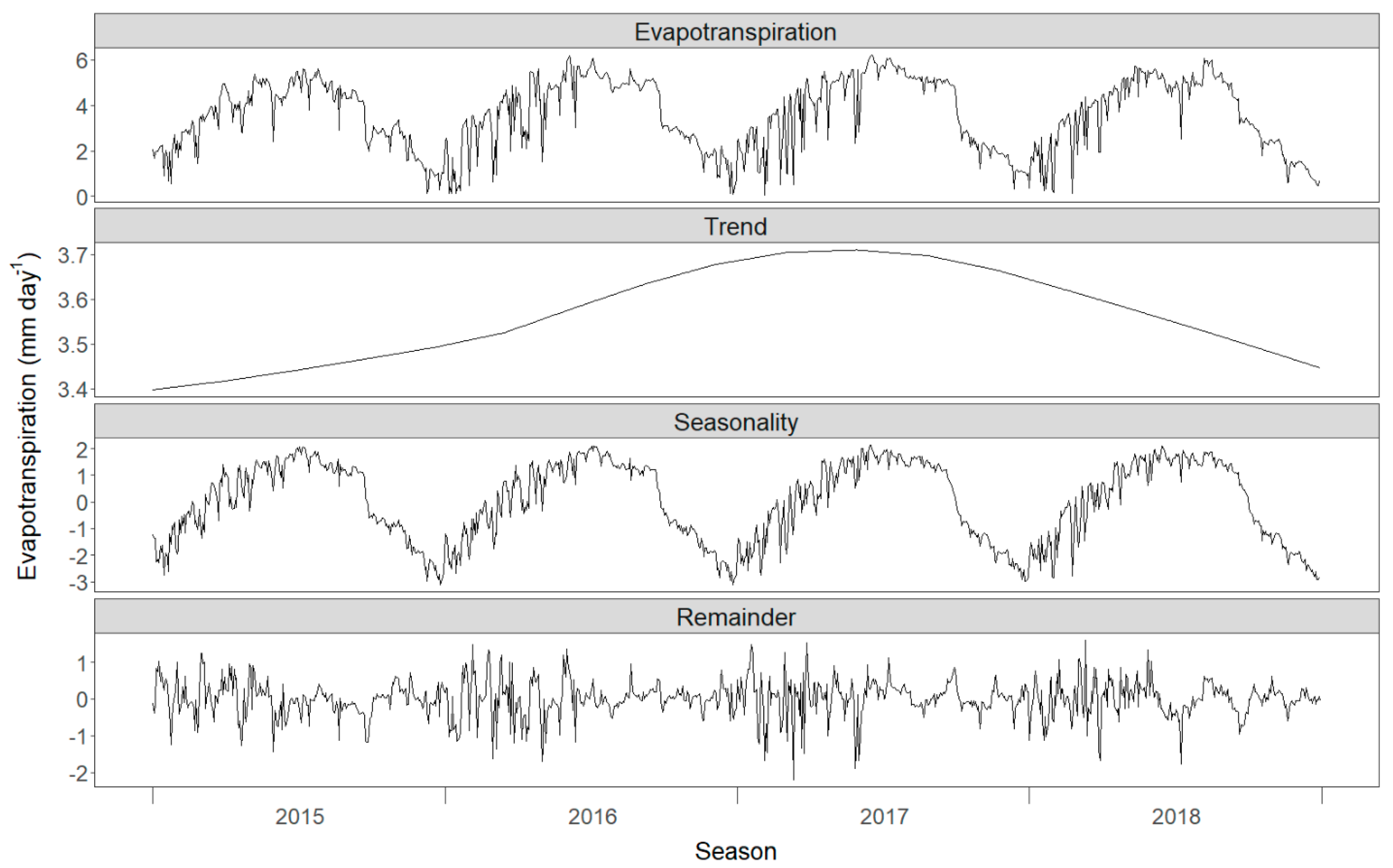
Time series representations: A time series is a set of observations, each recorded at a specific time [83]. A continuous time series consists of observations recorded continuously over a time interval. A time series may be displayed as a linear combination of components. These components provide information about patterns of change over time of latent processes composing the data [84] and include the trend, seasonality, and remainder. The trend represents low-frequency variations of the time series, including non-stationary, long-term inter-annual changes. The seasonal component accounts for the seasonal frequency in terms of cycles, in our case, cycles per growing season. The remainder component is the remaining variation (anomaly) in the data beyond the variation accounted by the seasonality and trend components [85]. It may be regarded as the local processes which cause variability among cycles, or shortest-term events [86], while in this present study, the shortest time unit is the daily scale. Decomposition of the time series allows for analyzing different underlying patterns in the data and has been previously used for quantifying multi-seasonal ET patterns [87]. The three components are affected by the inherent characteristics of the time series, such as length and frequency. However, as the suggested framework deals with comparative analysis among the time series of the pixels, it may work on any time period, as long as it consists of two cycles (growing seasons) or more. In other words, the meteorological conditions and effects will be similar for all pixels, regardless of the timeframe that is being used, and what matters is how the plants in each pixel respond to these conditions compared to other pixels. In this study, time-series decomposition was applied in order to analyze each timescale separately; namely, the multi-seasonal timescale (trend), the seasonal timescale (seasonality), and the daily timescale (remainder). The time series in the present project included 980 images. Therefore, each pixel had 980 daily values, and the decomposition was performed at the pixel level. The decomposition method that was used is the Seasonal and Trend decomposition using Loess (STL) [85] with seasonal window (the smoothing parameter for the seasonal filter) set to periodic (mean seasonal value), so that it was identical across all years. The trend window (the smoothing parameter of the trend) was set to the default 1.5 x period/1-(1.5/seasonal window). Figure A1, in the Appendix A, illustrates a time-series decomposition applied to a time series of one pixel. This process was conducted for all 334 pixels across the vineyard using the R package “stats” [88]. For the trend and remainder, the entire timeframe was used for the TSC procedure, while the seasonality component was reduced to one cycle using the “TSrepr” package in R [89].

Distance matrix: A scalar measure of dissimilarity between all pairs of observations (each observation is a time series of a specific pixel), or similarity matching, in this case each observation consists of daily values during four growing seasons. This whole-sequence matching considers the entire lengths of the time series during the distance calculation [82]. The dynamic time warping (DTW) algorithm is a technique applied to generate the distance matrix and was used to compute the similarity among time series (i.e., pixels). This dynamic programming technique is based on a non-linear warping function that eliminates timing differences between two temporal patterns by warping the time axis of one series so that the similar maximum values would coincide with each other. The time-normalized distance is then calculated as the minimized residual distance between the two series [90].

Clustering algorithm: Uses the distance matrix to group the data based on the similarities between each pair of pixels’ time series. In this study, we used the unsupervised fuzzy c-means (FCM) algorithm as the method of clustering. A fuzzy set has fuzzy boundaries where each element receives a degree of membership to each set. The data were partitioned into c fuzzy groups, and the FCM finds a cluster center (centroid) in each group such that the cost function of dissimilarity is minimized [91]. The fuzzification parameter, m, determines the degree of fuzziness in the clusters and, in this case, was set to 2, as conventionally suggested by most studies [92]. The FCM algorithm was applied to the data with $2\le c\le 6$, and the final number of groups was assigned based on the clustering result with the highest separation between within-cluster similarities and between-clusters dissimilarities. $c=6$ was defined as the maximum number of clusters since $MZ>6$ would not be practical for irrigation purposes. This partitioning evaluation was performed using the silhouette index, which measures the degree of similarity of each observation to its own cluster compared to other clusters [93]. It ranges from −1 and 1, while higher values indicate a stronger match to the assigned cluster. The average silhouette width (ASW) for the observations was computed using the “cluster” R package [94].

Time-series clustering maps: The outcomes, or output, of the TSC were maps composed of different clusters, while each pixel was assigned to a specific cluster. For each of the three components, the TSC map represented the spatial pattern of temporal similarities among different pixels. The trend TSC map illustrated the long-term, inter-seasonal pattern of change for each group of pixels. The seasonality TSC map represented the seasonal similarity among each group of pixels, and the remainder TSC map displayed the daily within-field spatial pattern according to the dissimilarities between the different clusters. The TSC based on DTW was applied using “dtwclust” package in R [95]. Corresponding plots of the time series for each component were also provided to show the dynamic patterns in time for each cluster. An additional difference plot among the values of the different TSC was presented to show the magnitude of dissimilarity among the clusters using the R packages “reshape2” [96], “data.table” [97], “RStoolbox [98], and “ggplot2” [99].

2.4. Precipitation and Irrigation Data Analysis

The irrigation regime and precipitation amount (mm) were examined in an attempt to explain the ET trend pattern. The spring precipitation values from February until June were therefore extracted from the meteorological station located in the vineyard. The accumulated precipitation was calculated, as well as the number of days with rainfall events. In addition, to complement the total water input to the vineyard, the amounts of irrigation per growing season were calculated. Finally, a sum of irrigation and precipitation amounts was provided for each growing season.

2.5. Assessment of Spatial Similarity among TSC Maps

To assess the degree of spatial pattern similarity among the three TSC maps, the V-Measure of spatial association between regionalizations [100] was applied. A regionalization is a segmentation of the map into a set of single-connected units. The maps may have areas of disjointed parts. The V-measure is an entropy-based measure that defines the distance from a perfect cluster-matching of two thematic maps, which relies on the homogeneity and completeness measures of two discrete maps. A clustering outcome satisfies homogeneity if all cluster domains contain only data points that are members of a single class. Completeness occurs when all the data pixels that are members of a given group are elements of the same cluster. Homogeneity and completeness are symmetrical measures that compose the V-Measure when averaging them using a harmonic mean [100,101]. Both homogeneity and completeness have values between 0 and 1, resulting in the same scale for the V-Measure. This assessment was applied for all pairs of TSC maps, resulting in three different assessments of spatial associations, using the “sabre” R package [100].

2.6. Influence of Field Attributes on ET Spatial Clustering Patterns

To comply with specific objective (3) and assess the rank of impact of different environmental variables within the vineyard on ET levels on different time scales, a random forest (RF) classifier was used. RF is based on a combination of tree classifiers, each generated using a random vector that is sampled independently from the input vector. Each tree casts a unit vote for the most popular class to classify an input vector [102]. Based on studies conducted for the past two decades, RF yields reliable classifications using predictions from an ensemble of decision trees and may be used for ranking the variables with the highest ability to partition the target classes. It is a non-parametric supervised model which creates trees by drawing a subset of training samples through replacement [103]. In this study, the environmental variables detailed in Section 2.2 (Figure 3) were evaluated for their relative importance to each ET-TSC map. The data were randomly partitioned with no iterations into training and testing using a ratio of 70% and 30%, respectively. The RF algorithm was applied on the training set, after which a prediction over the testing set was performed for evaluation of the model’s performance. The results were recorded, including the training error rate and error matrix, and the testing prediction accuracy in % and Kappa coefficient. This procedure was applied using the “RandomForest” package in R [104]. The representation of the results was enabled using the R packages “dplyr” [105], cowplot [106], and “ggplot2” [99].

2.7. Effect of ET on Yield

To estimate the extent to which the variability of the yield is explained by the two MZs of each component (trend, seasonality, and remainder) based on the TSC maps and the remainder, we used analysis of variance (ANOVA). ANOVA may be used after meeting a set of assumptions, one of which specifies that the observations should be drawn randomly and independently of each other. In attributes that are spatially autocorrelated, information redundancy is implied, and the duplication of information should be reduced to a minimum [107]. To draw a set of random observations that does not consist of spatial dependence, a minimum distance between observations was defined. Finding the minimum distance was enabled by computing the spatial structure variation with distance using an empirical semivariogram for the yield (Figure 4) [108]. An empirical semivariogram plots half the squared difference (i.e., semivariance) between any two observations against their actual distance, averaged for predefined bins (distance classes). The semivariogram consists of parameters defining its structure, including the range, specifying the maximum distance at which pairs of observations display spatial dependence. The model semivariogram assumes that there is no spatial autocorrelation for distances larger than the range [109]. The model semivariogram was computed using the R package “automap” [110] and the range was used as a minimum distance threshold to extract a random sample of the yield attribute, using the R package “spatialEco” [111]. The selected observations were then used for applying one-way ANOVA with the clusters used as the categorical variable and the yield as the dependent variable. If c > 2, a post-hoc test would be carried out to determine the differences among all pairs of clusters. It should be noted that for c = 2 an unpaired t-test may also be performed. The ANOVA assumptions of normality and homogeneity of variance across groups were tested using the Shapiro-Wilk Normality Test and the Levene’s Test, respectively. The procedure was applied using the R packages “raster” [62], “stats” [88], and “car” [112].

3. Results

3.1. Time-Series Clustering

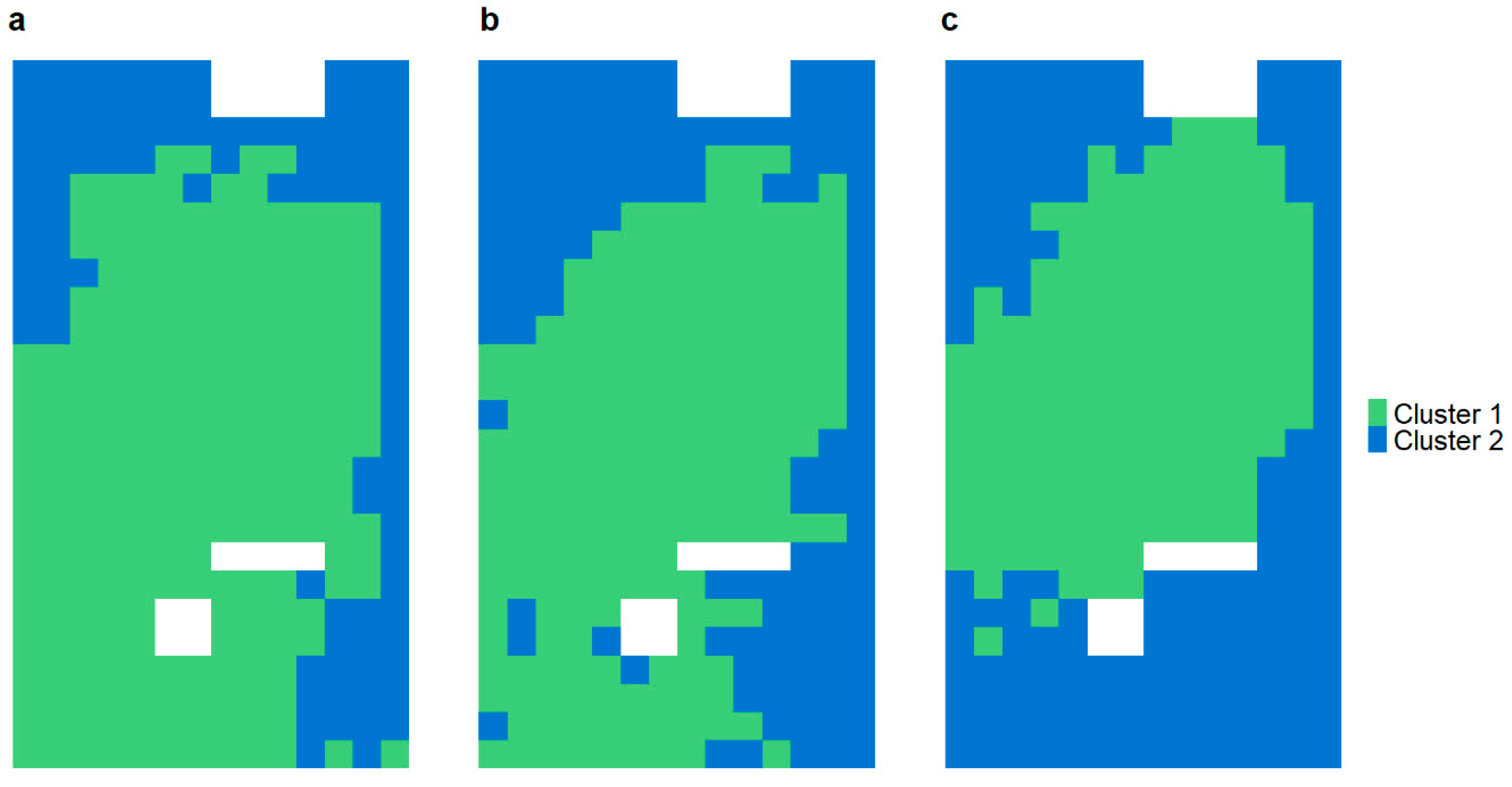
The highest ASW values for all decomposed components were achieved when applying FCM using c = 2, resulting in ASW of 0.53, 0.28, and 0.06 for the trend, seasonality, and remainder, respectively. Consequently, the TSC maps for each of the components were partitioned into two clusters (Figure 5). The clusters present an overall spatial uniformity with very little fragmentation for all cases. The areal coverage ratio between the clusters for the TSC maps was similar for the trend and seasonality components, with 70% and 30% of the area assigned to clusters 1 and 2, respectively, for the trend component, and 60% and 40% of the area assigned to clusters 1 and 2, respectively, for the seasonality component. The remainder TSC map showed a ratio of 51.5 and 48.5% areal coverage for clusters 1 and 2, respectively.

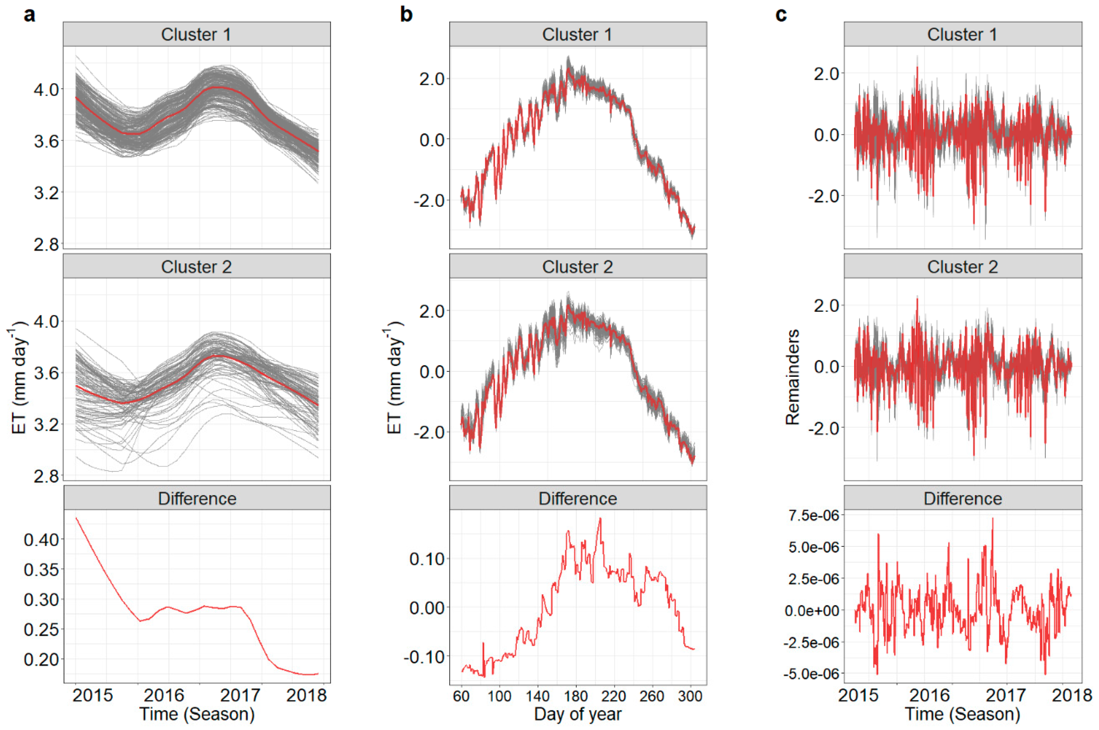
Figure 6 shows corresponding plots to the clusters illustrated in Figure 5, which demonstrate the characteristics and dynamics of the time series of each cluster for each component. Additionally, a third plot shows the difference between the centroids of both clusters to emphasize the dissimilarity between them. For the trend TSC (Figure 6a), the difference plot shows that the highest variation occurred during the 2015 growing season, where Cluster 1 had higher ET values, on average, and the difference ranged between 0.5 mm day⁻¹ in the beginning of the growing season and 0.26 mm day⁻¹ at the end of the season. During 2016 and 2017, the difference was constant around 0.27 mm day⁻¹, and in 2018 the difference was the lowest, with Cluster 1 having higher values of less than 0.2 mm day⁻¹ than Cluster 2. For the seasonality time series (Figure 6b), the differences throughout the season vary greatly, while the beginning and the end of the growing season were characterized by very low differences. During July and August, Cluster 1 had ET levels of 0.2 mm day⁻¹ higher than Cluster 2. Lastly, the remainder component (Figure 6c) showed high variability with variations of up to 2 mm day⁻¹. Clusters 1 and 2 showed no differences.

3.2. Irrigation and Precipitation

The amounts of irrigation and precipitation are detailed in

Table 1. Levels of precipitation during the spring (February-June) and irrigation in the vineyard during the four growing seasons.

Growing Season	Total Irrigation (mm)	Total Spring Precipitation (mm)	Number of Rainy Days	Sum of Irrigation and Precipitation (mm)
2015	491.03	101.85	14	592.89
2016	479.87	114.33	18	594.20
2017	300	300.23	35	600.23
2018	306.69	226.82	23	533.51

. During 2015 and 2016, the total amount of precipitation (mm) from February to June was much lower than during 2017 and 2018 (about 102, 114, 300, and 227 mm in 2015, 2016, 2017, and 2018, respectively). Consequently, the irrigation inputs to the vineyard were lower during the periods that experienced higher precipitation levels (i.e., 2017 & 2018). The 2015 and 2016 spring rainfall events were very few, while 2015 experienced 14 precipitation events during the spring, which was the lowest number of rainfall days recorded during the research period.

3.3. Assessment of Spatial Similarity among TSC Maps

The V-Measure of spatial association between regionalizations was applied to all pairs of TSC maps. The TSC maps of seasonality and trend showed higher similarity in their spatial patterns than each of these TSC maps with the remainder TSC map (

Table 2. V-measure of spatial association between regionalizations among the time-series clustering maps for each pair of time-series components. TSC stands for time-series clustering.

First Map	Second Map	Homogeneity	Completeness	V-Measure
seasonality TSC	Remainder TSC	0.29	0.28	0.29
seasonality TSC	Trend TSC	0.46	0.51	0.49
Remainders TSC	Trend TSC	0.19	0.22	0.2

).

3.4. Influence of Field Attributes on ET Spatial Clustering Patterns

The RF algorithm was applied three times and included the dataset of the six environmental variables (Figure 3), and each one of the three TSC maps. The application of RF enabled the generation of a classification model where the cluster map for each component served as the dependent variable and the six covariates received a rank of their relative importance to the clustering maps. Overall, the performance levels for the three RF models were high (

Table 3. Random forest model assessment for each time-series clustering map as the response variable.

Component (Time-Series Clustering)	Trend	Seasonality	Remainder
Error rate (%) (training)	14.62	15.57	17.92
Confusion matrix – class 1 error (training)	0.05	0.09	0.15
Confusion matrix – class 2 error (training)	0.39	0.26	0.20
Prediction accuracy (%) (testing)	89.34	86.89	86.07
Prediction accuracy (Kappa) (testing)	0.75	0.72	0.72

), with overall prediction accuracy > 86% based on the error-matrix for the test set. The model for the trend TSC map had the lowest error rate for the training model, as well as the highest prediction accuracy for the testing model, followed by the seasonality and remainder.

The most influencing covariate according to mean decrease in accuracy was soil type for the trend and seasonality, followed by elevation (Figure 7). The northness and slope were ranked third and fourth in their degree of importance. The remainder classification, however, showed strong effects of northness, followed by elevation and soil type.

3.5. Effect of ET on Yield

The Gaussian model semivariogram was constructed using a range of 55.5 m that was used as the minimum distance threshold for the random sampling of yield and the TSC maps. A total of 65 samples were extracted. The mean yield value for the entire vineyard was 9.94 ton ha-1, while the sample mean was 9.92 ton ha-1, with a non-significant difference (an unpaired t-test result of t = −0.04, p = 0.97) that ensured that the sample reliably represented the yield for the entire vineyard. ANOVA was carried out after meeting its assumptions, and the findings (

Table 4. Results for the ANOVA analysis determining the differences between yield levels in the clusters of each time-series clustering map, based on 65 sample points. The yield data were derived by a weighing harvesting machine on 22 August 2016.

Component (Time-Series Clustering)	Mean Yield Cluster 1 (ton ha−1)	Mean Yield Cluster 2 (ton ha−1)	F-Value	p-Value
Trend	10.52	8.57	6.82	0.01
Seasonality	11.09	8.36	20.21	<0.001
Remainders	11.2	8.92	13.76	<0.001

) show that the clusters for the three TSC maps were able to differentiate the levels of yield in the vineyard with statistically significant differences between cluster 1 and 2 for all components. The differences between the mean yield values for the two clusters were the highest for the seasonality TSC map, as well as the difference in variability of yield levels between the two clusters. For Cluster 1, the SD was 2.51, 2.11, and 2.4 ton ha-1 for the trend, seasonality, and remainders, respectively, and the corresponding values for Cluster 2 were 2.86, 2.76, and 2.58 ton ha-1.

4. Discussion

This study focused on quantifying the spatial and temporal patterns of ET in a Pinot noir commercial vineyard in California. The framework follows a holistic approach that considered multiple effects of environmental variables, meteorological factors, and different temporal scales to understand the spatial and temporal patterns of ET in the vineyard and partition their characteristics at multiple time scales according to time-series similarities. Each pixel in the dataset included 980 values, representing daily ET levels during four consecutive growing seasons. To analyze the similarities among the time series of the vineyard pixels, a TSC method was applied to each of three time-series components: long-term trend, seasonality, and remainder, which was regarded as the daily variation of the time series. Time-series analysis techniques are widely applied to ET data, due to their enabling long-term records and spatial coverage. Many studies use various techniques of time-series decomposition of ET for forecasting purposes [87,113]. Some used ET for time-series clustering. [114] found that a fuzzy framework for clustering of ET time-series in space was effective for delineating homogeneous ET_o regions. [115] used hierarchical time-series clustering of ET based on images acquired from multiple satellites across an entire agricultural river basin. Combining these two approaches resulted in TSC for each time-series component, and enabled us to further explore the spatial characteristics of each time scale.

Decomposition into three time scales enabled us to distinguish between latent temporal dynamics. The processes that define each component vary with space, time, and underlying effects of meteorological conditions and the spatial variability of different attributes in the vineyard. Two clusters were delineated for each component, resulting in TSC maps (Figure 5) that may also be viewed as the partitioning of the vineyard into MZs for precision irrigation purposes. The remainder clustering was very poor (ASW=0.11), which indicates strong similarities among the two clusters. The trend and seasonality TSC maps were found to have a stronger similarity of their spatial patterns than the remainder TSC (Table 2). The supporting plots of ET values for each cluster (Figure 6) may assist in defining the water stress levels of each MZ, as well as the similarities within each MZ. The trend and seasonality plots (Figure 6a,b) uncover the ET differences between the clusters, and the findings show that Cluster 1 had consistently higher ET values throughout the growing season and at a multi-seasonal time scale. During 2017 the ET levels were the highest across the entire vineyard, possibly due to high precipitation amounts. The difference between the cluster centroids enabled investigation of the effect of the meteorological conditions on each cluster’s temporal variability during different time scales. The large difference between the two MZs in the trend component (Figure 6a) may be attributed to seasonal variations in spring precipitation events and irrigation amounts (Table 1). These variations might explain the high trend differences among the MZs during 2015. Although the vineyards had received a similar amount of water in terms of rainfall and irrigation inputs, lower differences between MZs were found when spring precipitation levels and a number of rainfall days were higher (2016, 2017). During 2018, the total water input to the vineyard was the lowest, resulting in overall lower ET levels in both MZs, as well as a low difference (~0.2 mmday⁻¹). A possible explanation could be that higher levels of water availability in the vineyard during the early stages of the season cause a developed and more efficient system of hydraulic conductivity in the grapevines, which in turn become severely stressed towards the end of the growing season [116]. The performance of the RF models for the three components was satisfying (Table 3) and the results of these models (Figure 7) defined the soil type as the most influential static variable affecting ET clustering for the trend and seasonality components. Spring rainfall events highly influence soil moisture content, while the distribution of water input throughout more rainfall events helps to maintain higher soil moisture levels [117] and correspondingly increase water availability to the plants [118]. Additionally, areas with higher elevation levels in the vineyard were characterized by lower ET levels at long-term time scales and during the growing season. Lower, more homogeneous levels of altitudes are related to higher silt and clay content [119], thus allowing for water to be restored in the soil, prevent leakage downhill through both runoff and underground flow, provide better conditions for higher contents of soil moisture [120], and increase the availability of water to the grapevines.

The plots showing the differences in ET levels of the seasonality component (Figure 6b) enabled exploration of the seasonal dynamics of variation in space. During the beginning of the growing season when the canopy area was small, the differences in ET levels were negligible. In early May, the discrepancies increased, reaching a gap of 0.2 mm day⁻¹ during July. During this phenological stage (bunch closure until veraison), the canopy cover stabilized. After veraison, ET levels were constantly high until the plant suffered from leaf senescence and physiological deterioration, reducing the ability of the stomata to mediate photosynthetic activity [121]. During this phenological stage, the differences were more enhanced due to variation in soil types of each MZ. The vines composing Cluster 1 are located on top of the Kimball silt loam soil group. These are deep soils with moderate water holding capacity. The vines in Cluster 2 were planted on top of shallower soils with low water holding capacity that do not sustain water availability to the plant as efficiently as the Kimball silt loam. Therefore, during June and July when temperature levels are highest, the differences between the two clusters were more pronounced. These findings correspond to previous studies showing that decreasing levels of soil saturation are characterized by higher spatial variability [122] and that higher spatial variability in ET levels was found during the summer season [123].

All components were subjected to impact by the northness, which was the strongest contributor for the remainder. North- and northwest-facing slopes were associated with higher ET levels. These findings correspond with previous studies that demonstrated that south-facing slopes are subjected to stronger radiation [124], therefore lowering the soil moisture content and affecting water availability to the plant and plant density [59,125]. Denser vegetation then transpires more, leading to higher ET values.

Overall, the remainder levels of each pixel were unique and did not enable an accurate differentiation between pixels. The remainder differences were negligible and spanned around zero (Figure 6c). Decomposition of crop ET (i.e., ET_c) in a Mediterranean vineyard also found that fluctuations in ET values are commonly stronger in early spring (Figure A1) due to highly variable meteorological conditions [87], affecting the ET levels on a daily scale. The extent of influence of the various environmental factors, both meteorological and spatially varying attributes, is site-specific. Although the relations between different attributes and plant conditions are well-documented, the relative importance of these attributes is unique in each agricultural plot.

ET levels during the season may be associated with yield levels, and the analysis of yield against MZ for each component may support this claim. The ANOVA results show that all TSC maps were able to significantly distinguish between yield values spatially. The difference between the two MZs for each component ranged between 1.95 and 2.73 ton ha⁻¹.

Overall, the daily scale was not optimal for defining MZs and quantifying their underlying processes and averaged temporal dynamics. Practical use of this framework for irrigation modeling would require relating to ET processes at coarser time scales, such as the entire growing season, or during a multi-seasonal timeframe (long-term trend) for optimal differentiation of the vineyard. Site-specific management based on the spatial variability of water stress has been studied for the past years [126,127,128]. Irrigation protocols may benefit from the proposed technique to quantify water stress, both temporally and spatially. Site-specific management for irrigation purposes may be applied while considering the spatial variability of ET time series, along with a supporting quantification of ET levels in each MZ at multiple time scales. It is worth noting that effective irrigation management in the field requires spatially homogeneous clusters and will therefore benefit from undergoing a smoothness procedure prior to application that will generate non-fragmented clusters in space.

Finally, a similar analysis was conducted using the ratio between ET assessment and reference ET (ETo), which related ET to a living reference crop of grass [129]. This ET-ETo ratio (fRET) represents the crop ET while masking out the meteorological conditions and effects and is referred to as the moisture stress factor [36]. The spatial dynamics of fRET were similar to the ET analysis and therefore were not illustrated in this manuscript; however, fRET should also be examined for irrigation purposes while considering time-space-based irrigation application.

5. Conclusions

The research presented in this manuscript was aimed at defining spatial and temporal patterns of ET within a vineyard, relying on a data fusion framework based on images from multiple satellite sensors. The findings show that the long-term trend and seasonal patterns of the time series provided a similar spatial distribution of pixel similarity. The area of the vineyard planted on top of a silt loam soil had strong within-group similarities and better conditions to consume more water. Overall, the grapevines had a strong response to the altitude and soil characteristics in the vineyard, which was reflected in the temporal dynamics of their ET levels. This spatial heterogeneity also affected yield patterns across the vineyard, while grapevines with higher ET levels were also generally associated with higher levels of yield. The suggested framework may assist in defining site-specific irrigation protocols that consist of delineating the vineyard into zones with spatial similarities. For each zone, the temporal characteristics of ET may also be available, providing a complete illustration of the vineyard’s water stress conditions, both spatially and temporally, at different time scales.

With new, high-resolution satellite imagery options, such as Sentinel-2 and Venus, this analysis may be applied at a higher spatial resolution, increasing the detail level of spatial heterogeneity. Moreover, with a higher number of pixels available for a specific vineyard, the statistical time-series analysis would be stronger.

The application of the framework presented in the present paper is not limited to vineyards. It may be used for other agricultural practices, based on other data sources and different variables that quantify plant conditions or soil attributes with regular time intervals. The scope of the framework could be extended to other fields of research, such as environmental phenomena, epidemiology, spatially dependent economic attributes (e.g., consumption dynamics over space), and more.

References

1. Romero, M.; Luo, Y.; Su, B.; Fuentes, S. Vineyard water status estimation using multispectral imagery from an UAV platform and machine learning algorithms for irrigation scheduling management. Comput. Electron. Agric. 2018, 147, 109–117. [Google Scholar] [CrossRef]
2. Chai, Q.; Gan, Y.; Zhao, C.; Xu, H.L.; Waskom, R.M.; Niu, Y.; Siddique, K.H.M. Regulated deficit irrigation for crop production under drought stress. A review. Agron. Sustain. Dev. 2016, 36, 1–21. [Google Scholar] [CrossRef] [Green Version]
3. González Perea, R.; Daccache, A.; Rodríguez Díaz, J.A.; Camacho Poyato, E.; Knox, J.W. Modelling impacts of precision irrigation on crop yield and in-field water management. Precis. Agric. 2018, 19, 497–512. [Google Scholar] [CrossRef]
4. Galindo, A.; Collado-González, J.; Griñán, I.; Corell, M.; Centeno, A.; Martín-Palomo, M.J.; Girón, I.F.; Rodríguez, P.; Cruz, Z.N.; Memmi, H.; et al. Deficit irrigation and emerging fruit crops as a strategy to save water in Mediterranean semiarid agrosystems. Agric. Water Manag. 2018, 202, 311–324. [Google Scholar] [CrossRef]
5. Boutraa, T. Improvement of water use efficiency in irrigated agriculture: A Review. J. Agron. 2010, 9, 1–8. [Google Scholar] [CrossRef]
6. Clemmens, A.J.; Dedrick, A.R. Irrigation Techniques and Evaluations; Springer: Berlin/Heidelberg, Germany, 1994; pp. 64–103. [Google Scholar]
7. Rud, R.; Cohen, Y.; Alchanatis, V.; Levi, A.; Brikman, R.; Shenderey, C.; Heuer, B.; Markovitch, T.; Dar, Z.; Rosen, C.; et al. Crop water stress index derived from multi-year ground and aerial thermal images as an indicator of potato water status. Precis. Agric. 2014, 15, 273–289. [Google Scholar] [CrossRef]
8. Van Leeuwen, C.; Seguin, G. The concept of terroir in viticulture. J. Wine Res. 2006, 17, 1–10. [Google Scholar] [CrossRef]
9. Farid, H.U.; Bakhsh, A.; Ahmad, N.; Ahmad, A.; Mahmood-Khan, Z. Delineating site-specific management zones for precision agriculture. J. Agric. Sci. 2016, 154, 273–286. [Google Scholar] [CrossRef]
10. Nawar, S.; Corstanje, R.; Halcro, G.; Mulla, D.; Mouazen, A.M. Delineation of Soil Management Zones for Variable-Rate Fertilization: A Review. In Advances in Agronomy; Academic Press Inc.: Cambridge, MA, USA, 2017; Volume 143, pp. 175–245. [Google Scholar]
11. Haghverdi, A.; Leib, B.G.; Washington-Allen, R.A.; Ayers, P.D.; Buschermohle, M.J. Perspectives on delineating management zones for variable rate irrigation. Comput. Electron. Agric. 2015, 117, 154–167. [Google Scholar] [CrossRef]
12. Méndez-Vázquez, L.J.; Lira-Noriega, A.; Lasa-Covarrubias, R.; Cerdeira-Estrada, S. Delineation of site-specific management zones for pest control purposes: Exploring precision agriculture and species distribution modeling approaches. Comput. Electron. Agric. 2019, 167, 105101. [Google Scholar] [CrossRef]
13. Pádua, L.; Marques, P.; Adão, T.; Guimarães, N.; Sousa, A.; Peres, E.; Sousa, J.J. Vineyard Variability Analysis through UAV-Based Vigour Maps to Assess Climate Change Impacts. Agronomy 2019, 9, 581. [Google Scholar] [CrossRef] [Green Version]
14. Bahat, I.; Netzer, Y.; Ben-Gal, A.; Grünzweig, J.M.; Peeters, A.; Cohen, Y. Comparison of water potential and yield parameters under uniform and variable rate drip irrigation in a cabernet sauvignon vineyard. In Proceedings of the Precision Agriculture 2019-Papers Presented at the 12th European Conference on Precision Agriculture, ECPA, Montpellier, France, 8–11 July 2019; Wageningen Academic Publishers: Montpellier, France, 2019; pp. 125–131. [Google Scholar]
15. Ohana-Levi, N.; Bahat, I.; Peeters, A.; Shtein, A.; Netzer, Y.; Cohen, Y.; Ben-Gal, A. A weighted multivariate spatial clustering model to determine irrigation management zones. Comput. Electron. Agric. 2019, 162, 719–731. [Google Scholar] [CrossRef]
16. Allen, R.G.; Pereira, L.S.; Raes, D.; Smith, M. Crop Evapotranspiration-Guidelines for Computing Crop Water Requirements- Irrigation and Drainage Paper 56; FAO: Rome, Italy, 1998; Volume 56. [Google Scholar]
17. Williams, L.E.; Ayars, J.E. Grapevine water use and the crop coefficient are linear functions of the shaded area measured beneath the canopy. Agric. For. Meteorol. 2005, 132, 201–211. [Google Scholar] [CrossRef]
18. Massmann, A.; Gentine, P.; Lin, C. When Does Vapor Pressure Deficit Drive or Reduce Evapotranspiration? J. Adv. Model. Earth Syst. 2019, 11, 3305–3320. [Google Scholar] [CrossRef] [PubMed] [Green Version]
19. Lei, H.; Yang, D. Interannual and seasonal variability in evapotranspiration and energy partitioning over an irrigated cropland in the North China Plain. Agric. For. Meteorol. 2010, 150, 581–589. [Google Scholar] [CrossRef]
20. Payero, J.O.; Tarkalson, D.D.; Irmak, S.; Davison, D.; Petersen, J.L. Effect of irrigation amounts applied with subsurface drip irrigation on corn evapotranspiration, yield, water use efficiency, and dry matter production in a semiarid climate. Agric. Water Manag. 2008, 95, 895–908. [Google Scholar] [CrossRef] [Green Version]
21. Munitz, S.; Schwartz, A.; Netzer, Y. Water consumption, crop coefficient and leaf area relations of a Vitis vinifera cv. “Cabernet Sauvignon” vineyard. Agric. Water Manag. 2019, 219, 86–94. [Google Scholar] [CrossRef]
22. Williams, L.; Phene, C. Water use of mature Thompson Seedless grapevines in California. Irrig. Sci. 2003, 11–18. [Google Scholar] [CrossRef]
23. Picón-Toro, J.; González-Dugo, V.; Uriarte, D.; Mancha, L.A.; Testi, L. Effects of canopy size and water stress over the crop coefficient of a “Tempranillo” vineyard in south-western Spain. Irrig. Sci. 2012, 30, 419–432. [Google Scholar] [CrossRef] [Green Version]
24. Bastiaanssen, W.G.M.; Menenti, M.; Feddes, R.A.; Holtslag, A.A.M. A remote sensing surface energy balance algorithm for land (SEBAL): 1. Formulation. J. Hydrol. 1998, 212–213, 198–212. [Google Scholar] [CrossRef]
25. Su, Z. The Surface Energy Balance System (SEBS) for estimation of turbulent heat fluxes. Hydrol. Earth Syst. Sci. 2002, 6, 85–100. [Google Scholar] [CrossRef]
26. Allen, R.G.; Tasumi, M.; Trezza, R. Satellite-Based Energy Balance for Mapping Evapotranspiration with Internalized Calibration (METRIC)—Model. J. Irrig. Drain. Eng. 2007, 133, 380–394. [Google Scholar] [CrossRef]
27. Anderson, M.C.; Norman, J.M.; Diak, G.R.; Kustas, W.P.; Mecikalski, J.R. A two-source time-integrated model for estimating surface fluxes using thermal infrared remote sensing. Remote Sens. Environ. 1997, 60, 195–216. [Google Scholar] [CrossRef]
28. Bastiaanssen, W.G.M.; Pelgrum, H.; Wang, J.; Ma, Y.; Moreno, J.F.; Roerink, G.J.; Van Der Wal, T. A remote sensing surface energy balance algorithm for land (SEBAL): 2. Validation. J. Hydrol. 1998, 212–213, 213–229. [Google Scholar] [CrossRef]
29. Kustas, W.P.; Norman, J.M. Evaluation of soil and vegetation heat flux predictions using a simple two-source model with radiometric temperatures for partial canopy cover. Agric. For. Meteorol. 1999, 94, 13–29. [Google Scholar] [CrossRef]
30. Anderson, M.C.; Norman, J.M.; Mecikalski, J.R.; Otkin, J.A.; Kustas, W.P. A climatological study of evapotranspiration and moisture stress across the continental United States based on thermal remote sensing: 1. Model formulation. J. Geophys. Res. Atmos. 2007, 112. [Google Scholar] [CrossRef]
31. Norman, J.M.; Anderson, M.C.; Kustas, W.P.; French, A.N.; Mecikalski, J.; Torn, R.; Diak, G.R.; Schmugge, T.J.; Tanner, B.C.W. Remote sensing of surface energy fluxes at 10 1-m pixel resolutions. Water Resour. Res. 2003, 39. [Google Scholar] [CrossRef] [Green Version]
32. Anderson, M.C.; Norman, J.M.; Mecikalski, J.R.; Torn, R.D.; Kustas, W.P.; Basara, J.B. A Multiscale Remote Sensing Model for Disaggregating Regional Fluxes to Micrometeorological Scales. J. Hydrometeorol. 2004, 5, 343–363. [Google Scholar] [CrossRef]
33. Semmens, K.A.; Anderson, M.C.; Kustas, W.P.; Gao, F.; Alfieri, J.G.; McKee, L.; Prueger, J.H.; Hain, C.R.; Cammalleri, C.; Yang, Y.; et al. Monitoring daily evapotranspiration over two California vineyards using Landsat 8 in a multi-sensor data fusion approach. Remote Sens. Environ. 2016, 185, 155–170. [Google Scholar] [CrossRef] [Green Version]
34. Xia, T.; Kustas, W.P.; Anderson, M.C.; Alfieri, J.G.; Gao, F.; McKee, L.; Prueger, J.H.; Geli, H.M.E.; Neale, C.M.U.; Sanchez, L.; et al. Mapping evapotranspiration with high-resolution aircraft imagery over vineyards using one- and two-source modeling schemes. Hydrol. Earth Syst. Sci. 2016, 20, 1523–1545. [Google Scholar] [CrossRef] [Green Version]
35. Kustas, W.P.; Anderson, M.C.; Alfieri, J.G.; Knipper, K.; Torres-Rua, A.; Parry, C.K.; Nieto, H.; Agam, N.; White, W.A.; Gao, F.; et al. The Grape Remote Sensing Atmospheric Profile and Evapotranspiration Experiment. Bull. Am. Meteorol. Soc. 2018, 99, 1791–1812. [Google Scholar] [CrossRef] [Green Version]
36. Knipper, K.R.; Kustas, W.P.; Anderson, M.C.; Alfieri, J.G.; Prueger, J.H.; Hain, C.R.; Gao, F.; Yang, Y.; McKee, L.G.; Nieto, H.; et al. Evapotranspiration estimates derived using thermal-based satellite remote sensing and data fusion for irrigation management in California vineyards. Irrig. Sci. 2019, 37, 431–449. [Google Scholar] [CrossRef]
37. Knipper, K.R.; Kustas, W.P.; Anderson, M.C.; Alsina, M.M.; Hain, C.R.; Alfieri, J.G.; Prueger, J.H.; Gao, F.; McKee, L.G.; Sanchez, L.A. Using High-Spatiotemporal Thermal Satellite ET Retrievals for Operational Water Use and Stress Monitoring in a California Vineyard. Remote Sens. 2019, 11, 2124. [Google Scholar] [CrossRef] [Green Version]
38. Moran, M.S. Thermal infrared measurement as an indicator of plant ecosystem health. In Thermal Remote Sensing in Land Processes; Quattrochi, D., Luval, J., Eds.; CRC Press: Boca Raton, FL, USA, 2004; pp. 257–282. [Google Scholar]
39. Gao, F.; Masek, J.; Schwaller, M.; Hall, F. On the blending of the landsat and MODIS surface reflectance: Predicting daily landsat surface reflectance. IEEE Trans. Geosci. Remote Sens. 2006, 44, 2207–2218. [Google Scholar] [CrossRef]
40. Knipper, K.R.; Kustas, W.P.; Anderson, M.C.; Nieto, H.; Alfieri, J.G.; Prueger, J.H.; Hain, C.R.; Gao, F.; McKee, L.G.; Alsina, M.M.; et al. Using high-spatiotemporal thermal satellite ET retrievals to monitor water use over California vineyards of different climate, vine variety and trellis design. Agric. Water Manag. 2020, 241, 106361. [Google Scholar] [CrossRef]
41. Oliver, M.A. Geostatistical Applications for Precision Agriculture; Springer: Dordrecht, The Netherlands, 2010. [Google Scholar]
42. Zheng, Z.; Zhang, F.; Ma, F.; Chai, X.; Zhu, Z.; Shi, J.; Zhang, S. Spatiotemporal changes in soil salinity in a drip-irrigated field. Geoderma 2009, 149, 243–248. [Google Scholar] [CrossRef]
43. Rochette, P.; Desjardins, R.L.; Pattey, E. Spatial and temporal variability of soil respiration in agricultural fields. Can. J. Soil Sci. 1991, 71, 189–196. [Google Scholar] [CrossRef]
44. Straw, C.M.; Henry, G.M. Spatiotemporal variation of site-specific management units on natural turfgrass sports fields during dry down. Precis. Agric. 2018, 19, 395–420. [Google Scholar] [CrossRef]
45. Brown, J.C.; Kastens, J.H.; Coutinho, A.C.; de Castro Victoria, D.; Bishop, C.R. Classifying multiyear agricultural land use data from Mato Grosso using time-series MODIS vegetation index data. Remote Sens. Environ. 2013, 130, 39–50. [Google Scholar] [CrossRef] [Green Version]
46. Hill, M.J.; Donald, G.E. Estimating spatio-temporal patterns of agricultural productivity in fragmented landscapes using AVHRR NDVI time series. Remote Sens. Environ. 2003, 84, 367–384. [Google Scholar] [CrossRef]
47. Gao, F.; Morisette, J.T.; Wolfe, R.E.; Ederer, G.; Pedelty, J.; Masuoka, E.; Myneni, R.; Tan, B.; Nightingale, J. An algorithm to produce temporally and spatially continuous MODIS-LAI time series. IEEE Geosci. Remote Sens. Lett. 2008, 5, 60–64. [Google Scholar] [CrossRef]
48. Tagarakis, A.; Liakos, V.; Fountas, S.; Koundouras, S.; Gemtos, T.A. Management zones delineation using fuzzy clustering techniques in grapevines. Precis. Agric. 2013, 14, 18–39. [Google Scholar] [CrossRef]
49. Jiang, Q.; Fu, Q.; Wang, Z. Delineating site-specific irrigation management zones. Irrig. Drain. 2011, 60, 464–472. [Google Scholar] [CrossRef]
50. De Lannoy, G.J.M.; Verhoest, N.E.C.; Houser, P.R.; Gish, T.J.; Van Meirvenne, M. Spatial and temporal characteristics of soil moisture in an intensively monitored agricultural field (OPE3). J. Hydrol. 2006, 331, 719–730. [Google Scholar] [CrossRef] [Green Version]
51. Petitjean, F.; Inglada, J.; Gançarski, P. Satellite image time series analysis under time warping. IEEE Trans. Geosci. Remote Sens. 2012, 50, 3081–3095. [Google Scholar] [CrossRef]
52. Zhang, L.; Weng, Q.; Shao, Z. An evaluation of monthly impervious surface dynamics by fusing Landsat and MODIS time series in the Pearl River Delta, China, from 2000 to 2015. Remote Sens. Environ. 2017, 201, 99–114. [Google Scholar] [CrossRef]
53. Murolo, S.; Mancini, V.; Romanazzi, G. Spatial and temporal stolbur population structure in a cv. Chardonnay vineyard according to vmp1 gene characterization. Plant Pathol. 2014, 63, 700–707. [Google Scholar] [CrossRef]
54. McNaughton, K.G.; Spriggs, T.W. A mixed-layer model for regional evaporation. Boundary-Layer Meteorol. 1986, 34, 243–262. [Google Scholar] [CrossRef]
55. Kustas, W.P.; Diak, G.R.; Norman, J.M. Time difference methods for monitoring regional scale heat fluxes with remote sensing. In Land Surface Hydrology, Meteorology, and Climate: Observations and Modeling; Lakshmi, V., Albertson, J., Schaake, J., Eds.; American Geophysical Union (AGU): Washington, DC, USA, 2001. [Google Scholar]
56. Cammalleri, C.; Anderson, M.C.; Gao, F.; Hain, C.R.; Kustas, W.P. Mapping daily evapotranspiration at field scales over rainfed and irrigated agricultural areas using remote sensing data fusion. Agric. For. Meteorol. 2014, 186, 1–11. [Google Scholar] [CrossRef] [Green Version]
57. Anderson, M.; Gao, F.; Knipper, K.; Hain, C.; Dulaney, W.; Baldocchi, D.; Eichelmann, E.; Hemes, K.; Yang, Y.; Medellin-Azuara, J.; et al. Field-Scale Assessment of Land and Water Use Change over the California Delta Using Remote Sensing. Remote Sens. 2018, 10, 889. [Google Scholar] [CrossRef] [Green Version]
58. Moritz, S.; Bartz-Beielstein, T. imputeTS: Time Series Missing Value Imputation in R. R J. 2017, 9, 207–218. [Google Scholar] [CrossRef] [Green Version]
59. Ohana-Levi, N.; Paz-Kagan, T.; Panov, N.; Peeters, A.; Tsoar, A.; Karnieli, A. Time series analysis of vegetation-cover response to environmental factors and residential development in a dryland region. GIScience Remote Sens. 2019, 56. [Google Scholar] [CrossRef] [Green Version]
60. Brunsell, N.A.; Ham, J.M.; Owensby, C.E. Assessing the multi-resolution information content of remotely sensed variables and elevation for evapotranspiration in a tall-grass prairie environment. Remote Sens. Environ. 2008, 112, 2977–2987. [Google Scholar] [CrossRef]
61. Horn, B.K.P. Hill Shading and the Reflectance Map. Proc. IEEE 1981, 69, 14–47. [Google Scholar] [CrossRef] [Green Version]
62. Hijmans, R.J. Raster: Geographic Data Analysis and Modeling. R Package Version 3.1-5 2020. Available online: https://CRAN.R-project.org/packa (accessed on 24 May 2020).
63. Mohanty, B.P.; Skaggs, T.H. Spatio-temporal evolution and time-stable characteristics of soil moisture within remote sensing footprints with varying soil, slope, and vegetation. Adv. Water Resour. 2001, 24, 1051–1067. [Google Scholar] [CrossRef]
64. Zolekar, R.B.; Bhagat, V.S. Multi-criteria land suitability analysis for agriculture in hilly zone: Remote sensing and GIS approach. Comput. Electron. Agric. 2015, 118, 300–321. [Google Scholar] [CrossRef]
65. Roberts, D.W. Ordination on the basis of fuzzy set theory. Vegetatio 1986, 66, 123–131. [Google Scholar] [CrossRef]
66. Jelaska, S.D.; Antonić, O.; Božić, M.; Križan, J.; Kušan, V. Responses of forest herbs to available understory light measured with hemispherical photographs in silver fir-beech forest in Croatia. Ecol. Modell. 2006, 194, 209–218. [Google Scholar] [CrossRef]
67. Ghosh, B.N.; Sharma, N.K.; Alam, N.M.; Singh, R.J.; Juyal, G.P. Elevation, slope aspect and integrated nutrient management effects on crop productivity and soil quality in North-west Himalayas, India. J. Mt. Sci. 2014, 11, 1208–1217. [Google Scholar] [CrossRef]
68. Metcalfe, P.; Beven, K.; Freer, J. Dynatopmodel: Implementation of the Dynamic TOPMODEL Hydrological Model. R Package Version 1.2.1 2018. Available online: https://CRAN.R-project.org/packa (accessed on 24 May 2020).
69. Petroselli, A.; Vessella, F.; Cavagnuolo, L.; Piovesan, G.; Schirone, B. Ecological behavior of Quercus suber and Quercus ilex inferred by topographic wetness index (TWI). Trees Struct. Funct. 2013, 27, 1201–1215. [Google Scholar] [CrossRef]
70. Pebesma, E.; Bivand, R.S. Classes and Methods for Spatial Data in R. R News 5 (2) 2005. Available online: https://cran.r-project.org/doc/R (accessed on 24 May 2020).
71. Dugas, W.A.; Meyer, W.S.; Barrs, H.D.; Fleetwood, R.J. Effects of soil type on soybean crop water use in weighing lysimeters—II. Root growth, soil water extraction and water-table contributions. Irrig. Sci. 1990, 11, 77–81. [Google Scholar] [CrossRef]
72. Rancho-Cordova. General Plan | City of Rancho Cordova; Rancho Cordova, CA, USA, 2006. [Google Scholar]
73. Abbas, G.; Qureshi, R.A.; Qureshi, S.J. Measurement of Soil Organic Matter in Different Lithology of Karachi. J. Biol. Sci. 2001, 1, 779–781. [Google Scholar] [CrossRef] [Green Version]
74. El Maayar, M.; Chen, J.M. Spatial scaling of evapotranspiration as affected by heterogeneities in vegetation, topography, and soil texture. Remote Sens. Environ. 2006, 102, 33–51. [Google Scholar] [CrossRef]
75. SSHCP, County of Sacramento, City of Galt, Sacramento County Water Agency, Sacramento Regional County Sanitation Agency, Sacramento Regional County Sanitation District, outheast Connector Joint Powers Authority. In South Sacramento Habitat Conservation Plan—South Sac HCP; Sacramento, CA, USA, 2018.
76. Edwards, R.D.; Rabey, D.F.; Kover, R.W. Soil Survey, Ventura Area, California; United States Department of Agriculture, Soil Conservation Service: Washington, DC, USA, 1970.
77. Braun, B.; Brzozowska, J. Natural conditions for the development of sustainable agriculture in the eastern part of the Łowicko-Błońska plain. Misc. Geogr. 2012, 16. [Google Scholar] [CrossRef] [Green Version]
78. USDA/NRCS National Elevation Data 30 Meter 2019. Available online: https://gdg.sc.egov.usda.gov/ (accessed on 24 May 2020).
79. USDA/NRCS Gridded Soil Survey Geographic (gSSURGO) by State 2019. Available online: https://gdg.sc.egov.usda.gov/ (accessed on 24 May 2020).
80. USGS State Geologic Maps 2005. Available online: https://www.usgs.gov/products/ma (accessed on 24 May 2020).
81. Whelan, B.M.; Mcbratney, A.B.; Minasny, B. Vesper 1.5-spatial prediction software for precision agriculture. In Proceedings of the 6th International Conference of Precision Agriculture, Madison, WI, USA, 14–17 July 2002; Wisconsin. Rust, R., Larson, W., Eds.; ASA/CSSA/SSSA: Madison, WI, USA, 2002. [Google Scholar]
82. Aghabozorgi, S.; Seyed Shirkhorshidi, A.; Ying Wah, T. Time-series clustering—A decade review. Inf. Syst. 2015. [Google Scholar] [CrossRef]
83. Brockwell, P.J.; Davis, R.A. Introduction to Time Series and Forecasting, 3rd ed.; Springer: New York, NY, USA, 2016; ISBN 978-3-319-29854-2. [Google Scholar]
84. West, M. Time series decomposition. Biometrika 1997, 84, 489–494. [Google Scholar] [CrossRef]
85. Cleveland, R.B.; Cleveland, W.S.; McRae, J.E.; Terpenning, I. STL: A Seasonal-Trend Decomposition Procedure Based on Loess. J. Off. Stat. 1990, 6, 3–33. [Google Scholar]
86. Lafare, A.E.A.; Peach, D.W.; Hughes, A.G. Use of seasonal trend decomposition to understand groundwater behaviour in the Permo-Triassic Sandstone aquifer, Eden Valley, UK. Hydrogeol. J. 2016, 24, 141–158. [Google Scholar] [CrossRef] [Green Version]
87. Ohana-Levi, N.; Munitz, S.; Ben-Gal, A.; Schwartz, A.; Peeters, A.; Netzer, Y. Multiseasonal grapevine water consumption – Drivers and forecasting. Agric. For. Meteorol. 2020, 280, 107796. [Google Scholar] [CrossRef]
88. R Core Team R: A Language and Environment for Statistical Computing 2020. Available online: https://www.R-project.org/ (accessed on 24 May 2020).
89. Laurinec, P. TSrepr R package: Time Series Representations. J. Open Source Softw. 2018, 3, 577. [Google Scholar] [CrossRef]
90. Sakoe, H.; Chiba, S. Dynamic Programming Algorithm Optimization for Spoken Word Recognition. IEEE Trans. Acoust. 1978, 26, 43–49. [Google Scholar] [CrossRef] [Green Version]
91. Aghabozorgi, S.; Wah, T.Y. Effective Clustering of Time-Series Data Using FCM. Int. J. Mach. Learn. Comput. 2014, 4, 170–176. [Google Scholar] [CrossRef] [Green Version]
92. Huang, M.; Xia, Z.; Wang, H.; Zeng, Q.; Wang, Q. The range of the value for the fuzzifier of the fuzzy c-means algorithm. Pattern Recognit. Lett. 2012, 33, 2280–2284. [Google Scholar] [CrossRef]
93. Rousseeuw, P.J. Silhouettes: A graphical aid to the interpretation and validation of cluster analysis. J. Comput. Appl. Math. 1987, 20, 53–65. [Google Scholar] [CrossRef] [Green Version]
94. Maechler, M.; Rousseeuw, P.J.; Struyf, A.; Hubert, M.; Hornik, K. Cluster: Cluster Analysis Basics and Extensions. R Package Version 2.1.0. 2019. Available online: https://svn.r-project.org/R-pack (accessed on 24 May 2020).
95. Sarda-Espinosa, A. Dtwclust: Time Series Clustering Along with Optimizations for the Dynamic Time Warping Distance. R Package Version 5.5.6. 2019. Available online: https://CRAN.R-project.org/packa (accessed on 24 May 2020).
96. Wickham, H. Reshaping data with the reshape package. J. Stat. Softw. 2007, 21, 1–20. [Google Scholar] [CrossRef]
97. Dowle, M.; Srinivasan, A. Data.table: Extension of “data.frame”. R Package Version 1.12.8. 2019. Available online: https://CRAN.R-project.org/packa (accessed on 24 May 2020).
98. Leutner, B.; Horning, N.; Schwalb-Willmann, J.; Hijmans, R.J. RStoolbox: Tools for Remote Sensing Data Analysis. R Package Version 0.2.6. 2019. Available online: https://CRAN.R-project.org/packa (accessed on 24 May 2020).
99. Wickham, H. Ggplot2: Elegant Graphics for Data Analysis; Springer: New York, NY, USA, 2016; ISBN 9780387981406. [Google Scholar]
100. Nowosad, J.; Stepinski, T.F. Spatial association between regionalizations using the information-theoretical V -measure. Int. J. Geogr. Inf. Sci. 2018, 32, 2386–2401. [Google Scholar] [CrossRef] [Green Version]
101. Rosenberg, A.; Hirschberg, J.B. V-Measure: A conditional entropy-based external cluster evaluation. In Proceedings of the 2007 Joint Conference on Empirical Methods in Natural Language Processing and Computational Natural Language Learning, Prague, Czech Republic, 28–30 June 2007; pp. 410–420. [Google Scholar]
102. Breiman, L. Random forests. Mach. Learn. 2001, 45, 5–32. [Google Scholar] [CrossRef] [Green Version]
103. Belgiu, M.; Drăgu, L. Random forest in remote sensing: A review of applications and future directions. ISPRS J. Photogramm. Remote Sens. 2016, 114, 24–31. [Google Scholar] [CrossRef]
104. Liaw, A.; Wiener, M. Classification and Regression by randomForest. R News 2002, 2, 18–22. [Google Scholar]
105. Wickham, H.; François, R.; Henry, L.; Müller, K. Dplyr: A Grammar of Data Manipulation. R Package Version 0.8.5. 2020. Available online: https://CRAN.R-project.org/packa (accessed on 24 May 2020).
106. Wilke, C.O. Cowplot: Streamlined Plot Theme and Plot Annotations for “ggplot2”. R Package Version 1.0.0. 2019. Available online: https://CRAN.R-project.org/packa (accessed on 24 May 2020).
107. Haining, R. Spatial Autocorrelation. In International Encyclopedia of the Social & Behavioral Sciences, 2nd ed.; Elsevier Inc.: Amsterdam, The Netherlands, 2015; pp. 105–110. ISBN 9780080970875. [Google Scholar]
108. Isaaks, H.B.; Srivastava, R.M. An Introduction to Applied Geostαtistics; Oxford University Press Inc.: New York, NY, USA, 1989; ISBN 0195050134. [Google Scholar]
109. Wagner, H.H. Spatial covariance in plant communities: Integrating ordination, geostatistics, and variance testing. Ecology 2003, 84, 1045–1057. [Google Scholar] [CrossRef] [Green Version]
110. Hiemstra, P.H.; Pebesma, E.J.; Twenhöfel, C.J.W.; Heuvelink, G.B.M. Real-time automatic interpolation of ambient gamma dose rates from the Dutch radioactivity monitoring network. Comput. Geosci. 2009, 35, 1711–1721. [Google Scholar] [CrossRef]
111. Evans, J.S. SpatialEco: Spatial Analysis and Modelling Utilities. R Package Version 1.3-1 2020. Available online: https://github.com/jeffreyevans/ (accessed on 24 May 2020).
112. Fox, J.; Weisberg, S. An R Companion to Applied Regression, 3rd ed.; Sage: Thousand Oaks, CA, USA, 2019. [Google Scholar]
113. Wang, W.G.; Luo, Y.F. Wavelet network model for Reference Crop Evapotranspiration forecasting. In Proceedings of the 2007 International Conference on Wavelet Analysis and Pattern Recognition, ICWAPR ’07, Beijing, China, 2–4 November 2007; Institute of Electrical and Electronics Engineers Inc.: Beijing, China, 2007; Volume 2, pp. 751–755. [Google Scholar]
114. Masanta, S.K.; Vemavarapu, S.V. Regionalization of evapotranspiration using fuzzy dynamic clustering approach. Part 1: Formation of regions in India. Int. J. Climatol. 2020, 40, 3514–3530. [Google Scholar] [CrossRef]
115. González-Dugo, M.P.; Escuin, S.; Cano, F.; Cifuentes, V.; Padilla, F.L.M.; Tirado, J.L.; Oyonarte, N.; Fernández, P.; Mateos, L. Monitoring evapotranspiration of irrigated crops using crop coefficients derived from time series of satellite images. II. Application on basin scale. Agric. Water Manag. 2013, 125, 92–104. [Google Scholar] [CrossRef]
116. Netzer, Y.; Munitz, S.; Shtein, I.; Schwartz, A. Structural memory in grapevines: Early season water availability affects late season drought stress severity. Eur. J. Agron. 2019, 105, 96–103. [Google Scholar] [CrossRef]
117. Aviad, Y.; Kutiel, H.; Lavee, H. Variation of Dry Days Since Last Rain (DDSLR) as a measure of dryness along a Mediterranean—Arid transect. J. Arid Environ. 2009, 73, 658–665. [Google Scholar] [CrossRef]
118. Kamara, S.I.; Jackson, I.J. A new soil-moisture based classification of raindays and drydays and its application to Sierra Leone. Theor. Appl. Climatol. 1997, 56, 199–213. [Google Scholar] [CrossRef]
119. Pachepsky, Y.A.; Timlin, D.J.; Rawls, W.J. Soil Water Retention as Related to Topographic Variables. Soil Sci. Soc. Am. J. 2001, 65, 1787–1795. [Google Scholar] [CrossRef]
120. Hébrard, O.; Voltz, M.; Andrieux, P.; Moussa, R. Spatio-temporal distribution of soil surface moisture in a heterogeneously farmed Mediterranean catchment. J. Hydrol. 2006, 329, 110–121. [Google Scholar] [CrossRef]
121. Ohana-Levi, N.; Munitz, S.; Ben-Gal, A.; Netzer, Y. Evaluation of within-season grapevine evapotranspiration patterns and drivers using generalized additive models. Agric. Water Manag. 2020, 228, 105808. [Google Scholar] [CrossRef]
122. Nielsen, D.R.; Biggar, J.W.; Erh, K.T. Spatial variability of field-measured soil-water properties. Hilgardia 1973, 42, 215–259. [Google Scholar] [CrossRef] [Green Version]
123. Narasimhan, B.; Srinivasan, R. Development and evaluation of Soil Moisture Deficit Index (SMDI) and Evapotranspiration Deficit Index (ETDI) for agricultural drought monitoring. Agric. For. Meteorol. 2005, 133, 69–88. [Google Scholar] [CrossRef]
124. McCune, B.; Keon, D. Equations for potential annual direct incident radiation and heat load. J. Veg. Sci. 2002, 13, 603–606. [Google Scholar] [CrossRef]
125. Zaady, E.; Yonatan, R.; Shachak, M.; Perevolotsky, A. The Effects of Grazing on Abiotic and Biotic Parameters in a Semiarid Ecosystem: A Case Study from the Northern Negev Desert, Israel. Arid L. Res. Manag. 2001, 15, 245–261. [Google Scholar] [CrossRef]
126. Meron, M.; Tsipris, J.; Orlov, V.; Alchanatis, V.; Cohen, Y. Crop water stress mapping for site-specific irrigation by thermal imagery and artificial reference surfaces. Precis. Agric. 2010, 11, 148–162. [Google Scholar] [CrossRef]
127. O’Shaughnessy, S.A.; Evett, S.R.; Colaizzi, P.D. Dynamic prescription maps for site-specific variable rate irrigation of cotton. Agric. Water Manag. 2015, 159, 123–138. [Google Scholar] [CrossRef]
128. Cohen, Y.; Alchanatis, V.; Saranga, Y.; Rosenberg, O.; Sela, E.; Bosak, A. Mapping water status based on aerial thermal imagery: Comparison of methodologies for upscaling from a single leaf to commercial fields. Precis. Agric. 2017, 18, 801–822. [Google Scholar] [CrossRef]
129. Hargreaves, G.H. Defining and Using Reference Evapotranspiration. J. Irrig. Drain. Eng. 1994, 120, 1132–1139. [Google Scholar] [CrossRef]
Figure 1. The vineyard study site in Central Valley, California. The vineyard management complex and vernal pools within the area of the vineyard were masked out.
Remotesensing 12 02436 g001
Figure 2. Flowchart of the research framework.
Remotesensing 12 02436 g002
Figure 3. Environmental variables within the vineyard: (a) Elevation; (b) Slope; (c) Northness; (d) Topographic wetness index (TWI); (e) Soil type (HP stands for Hadselvill-Pentz complex); and (f) Lithology.
Remotesensing 12 02436 g003
Figure 4. A yield map derived by a weighing harvesting machine on 22 August 2016.
Remotesensing 12 02436 g004
Figure 5. Time-series clustering maps for each of the time-series components: (a) trend; (b) seasonality; and (c) remainder.
Remotesensing 12 02436 g005
Figure 6. Plots of time-series clusters and differences of centroids for each of the components: (a) trend; (b) seasonality; and (c) remainder. Red line defines the centroid of each cluster, while grey lines are the time series of the different pixels within each cluster.
Remotesensing 12 02436 g006
Figure 7. Variable importance according to mean decrease in accuracy of the six environmental variables for each time-series clustering map: (a) trend; (b) seasonality; and (c) remainder. The analysis was conducted using a random forest classifier. TWI stands for topographic wetness index.
Remotesensing 12 02436 g007