Super-Resolution of Sentinel-2 Imagery Using Generative Adversarial Networks

Abstract

Sentinel-2 satellites provide multi-spectral optical remote sensing images with four bands at 10 m of spatial resolution. These images, due to the open data distribution policy, are becoming an important resource for several applications. However, for small scale studies, the spatial detail of these images might not be sufficient. On the other hand, WorldView commercial satellites offer multi-spectral images with a very high spatial resolution, typically less than 2 m, but their use can be impractical for large areas or multi-temporal analysis due to their high cost. To exploit the free availability of Sentinel imagery, it is worth considering deep learning techniques for single-image super-resolution tasks, allowing the spatial enhancement of low-resolution (LR) images by recovering high-frequency details to produce high-resolution (HR) super-resolved images. In this work, we implement and train a model based on the Enhanced Super-Resolution Generative Adversarial Network (ESRGAN) with pairs of WorldView-Sentinel images to generate a super-resolved multispectral Sentinel-2 output with a scaling factor of 5. Our model, named RS-ESRGAN, removes the upsampling layers of the network to make it feasible to train with co-registered remote sensing images. Results obtained outperform state-of-the-art models using standard metrics like PSNR, SSIM, ERGAS, SAM and CC. Moreover, qualitative visual analysis shows spatial improvements as well as the preservation of the spectral information, allowing the super-resolved Sentinel-2 imagery to be used in studies requiring very high spatial resolution.

1. Introduction

Satellite remote sensing is used in various fields of application such as cartography, agriculture, environmental conservation, land use, urban planning, geology, natural hazards, hydrology, oceanography, atmosphere, climate, etc. In this context, a fundamental parameter to take into account when addressing a specific application is the spatial resolution.

With the recent launch of advanced instruments, the spatial resolution of satellite imagery has been enhanced. For instance, nowadays, WorldView-3/4 satellites [1] can collect 8-band multispectral data with 1.2 m of ground sample distance (GSD). Unfortunately, the cost to use such very high spatial resolution (VHSR) imagery can make it impractical when large areas have to be covered or if multi-temporal analysis have to be undertaken. Consequently, in these scenarios, it would be desirable to consider using open access data with acceptable spatial quality, like these provided by satellites such as Landsat or Sentinel. In particular, the Copernicus Sentinel-2 mission [2] comprises a constellation of two polar-orbiting satellites providing high revisit time and its Multi Spectral Instrument (MSI) records data in 13 spectral bands ranging from the visible to the shortwave infrared. This sensor acquires imagery at a spatial resolution of 10 m for the red, green, blue and near infrared channels. The previous technical characteristics make Sentinel-2 a very suitable candidate in a wide variety of applications related to the monitoring of land and coastal waters. Unfortunately, the excellent spatial detail available may not be sufficient for certain applications. In these challenging scenarios, the only solution is to purchase VHSR imagery acquired from commercial satellites or to consider lower altitude platforms, such as airplanes or drones. For this reason, in recent decades, the improvement of the spatial resolution of remote sensing images has been a very active research area with the aim of saving considerable amounts of money when addressing studies requiring periodic imagery or to cover large areas with such fine spatial detail.

One of the options to achieve a superior spatial resolution has been the application of pansharpening techniques. This enhancement of the multispectral (MS) or hyperspectral (HS) bands is feasible when the remote sensing platform includes an additional panchromatic (PAN) instrument providing better spatial resolution, typically with a scaling factor of 2 or 4. These methods aim to improve spatial quality without introducing spectral distortion in the original data. Quite a lot of pansharpening algorithms have been developed for MS and HS images in the last decades [3,4,5,6,7,8,9,10]. Recently, with the advent of deep learning (DL), new approaches have also been developed to address pansharpening [11,12,13,14,15,16], mainly, using architectures based on convolutional neural networks. As some platforms do not incorporate the supplementary PAN sensor, i.e. Sentinel-2, the alternative solution is the application of advanced super-resolution (SR) techniques to improve the spatial detail [17].

SR methods can be categorized into multi-image or single-image. Multi-image SR is based on the reconstruction of a higher resolution image by using a set of LR images, typically captured with different angles or at different satellite passes [18]. These LR images have sub-pixel misalignments and, thus, the land cover represented by a pixel in an image will not correspond exactly to that same pixel in a subsequent image. In practical applications it is not easy to obtain an adequate number of images from the same scene; therefore, single-image techniques are of greater interest. Regarding the single-image super-resolution domain, two different types of methods can be identified: supervised and unsupervised techniques. Even though unsupervised SR methods [19,20] have the benefit of not requiring a pair of input-target for a training dataset, its performance in remote sensing scenarios normally turns out to be quite limited because of the lack of spatial information in the LR data. In this context, supervised SR techniques can provide a more efficient approach using a training dataset to learn the relationships between high and low-resolution imagery.

In the last decade, some supervised SR techniques were developed based on dictionary approaches. In particular, Yang et al. [21,22], Dong et al. [23] or Gou et al. [24] provided effective solutions by considering sparse coding techniques. Pan et al. [25] used structural self-similarity and compressive sensing for super-resolution tasks. Other authors [26,27] used different image characterization spaces to achieve higher performance. However, in general, these approaches consider low-level features of the images.

Recently, deep learning has been applied to address the super-resolution topic [28]. For example, the use of high-level features from the optical data has provided significant improvement with the application of convolutional neural networks (CNN) for image super-resolution. Dong et al. introduced SRCNN [29], a three-layer CNN, and since then, many other CNN approaches have been explored [30,31,32,33].

On the other hand, lately, Generative Adversarial Networks (GANs) [34] have attracted an increasing attention from the research community, as the work of Ledig et al. [35] where they proposed SRGAN, a GAN based network that produced a more photo-realistic output but with lower quantitative metrics. It is a seminal work dealing with perceptual approach in SR. The generator’s architecture is composed of 16 residual blocks and 2 upsampling layers to produce a SR image with a scaling factor of 4. Besides, they divided the training stage by first training the generator and later in an adversarial mode combining adversarial and perceptual losses [36]. ESRGAN [37] is a model based on SRGAN that introduced some improvements like the use of a more complex and dense combination of residual layers in the generator and the removal of batch normalization layers, as they are prone to introduce artifacts. In addition, relativistic GAN [38] was used to improve the performance of the discriminator.

Super-resolution models based on CNNs face some challenges when applied to remote sensing, mainly related to the lack of training datasets. Ma et al. [39] proposed TGAN (Transferred Generative Adversarial Network) to solve the drawback of the poor quantity and quality of remote sensing data. Other authors like Haut et al. [40,41] and Lei et al. [42] downgraded public remote sensing images to form the LR-HR pairs and tested different network architectures. However, models trained only with synthetic LR-HR pairs tend to fail in generalization since the LR images are not only a consequence of Gaussian noise, blurring or compression artifacts [28,43]. More recently, Ma et al. [44] introduced DRGAN (Dense Residual Generative Adversarial Network) for the super-resolution of remote sensing imagery. Pouliot et al. [45] used a combination of Landsat (30 m GSD ) and Sentinel-2 (10 m GSD) imagery to train CNNs architectures for SR of Landsat imagery and Beaulieu et al. [46] have tested different CNNs and GANs networks with only one pair of Sentinel-2 (10 m GSD) and WorldView (2.5 m GSD) images with a scaling factor of 4. They have trained the models with 3 channels (Red, Green, and NIR) and the results were promising, especially using GAN-based networks. They believed that the radiometric and geometric differences between both satellites images could be an explanation of the low-value metrics obtained. Some authors have applied ESRGAN architectures as well, to solve different remote sensing SR problem applications [47,48]

This work focuses in the analysis of single-image supervised SR techniques using the DL paradigm. Specifically, we present a GAN-based super-resolution model to enhance the 10 m channels of the Sentinel-2 sensor to 2 m with a similar quality as produced by the WorldView satellite. The spatial enhancement process is achieved by exploiting the synergy existing in the spectral domain between the Sentinel-2 and Worldview-2/3 missions.

To train our model, image pairs coming from the Sentinel-2 and WorldView satellites were used. These LR and HR pairs are hard to obtain because, even though Sentinel imagery is freely available, the commercial aspect of the Worldview data and its non-systematic sensing of the Earth surface make it difficult to get enough image pairs to train the model. To overcome this problem, we decided to conduct the training in two stages. First, we used an artificially generated set of LR-HR image pairs with WorldView data to pre-train the model and, then, we fine-tuned the model using the WorldView-Sentinel pairs. To make it feasible to work with different satellite sources, we have removed the upsampling module of the ESRGAN architecture, as the images needed to be co-registered (see Section 3.2). Besides, the input and output layers were adapted to work with four bands (see Section 3.1). Another important contribution of our model is that before training, we standardize the data by channels, i.e. subtracting the mean and dividing by the standard deviation on each channel, in order to obtain an output image where the spectral characteristics of the LR Sentinel-2 image are preserved (see Section 4.1). Finally, once trained, our proposed RS-ESRGAN can be applied to obtain a super-resolved multispectral Sentinel-2 output with a scaling factor of 5.

The performances achieved have been compared to other super-resolution algorithms available in the literature in order to study the effectiveness of the proposed SR method, as well as to analyze the spectral/spatial quality trade-off obtained.

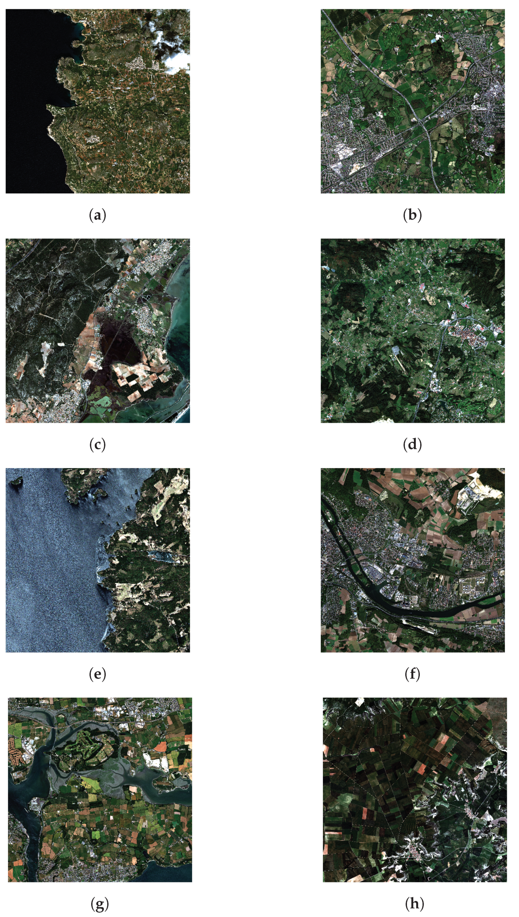
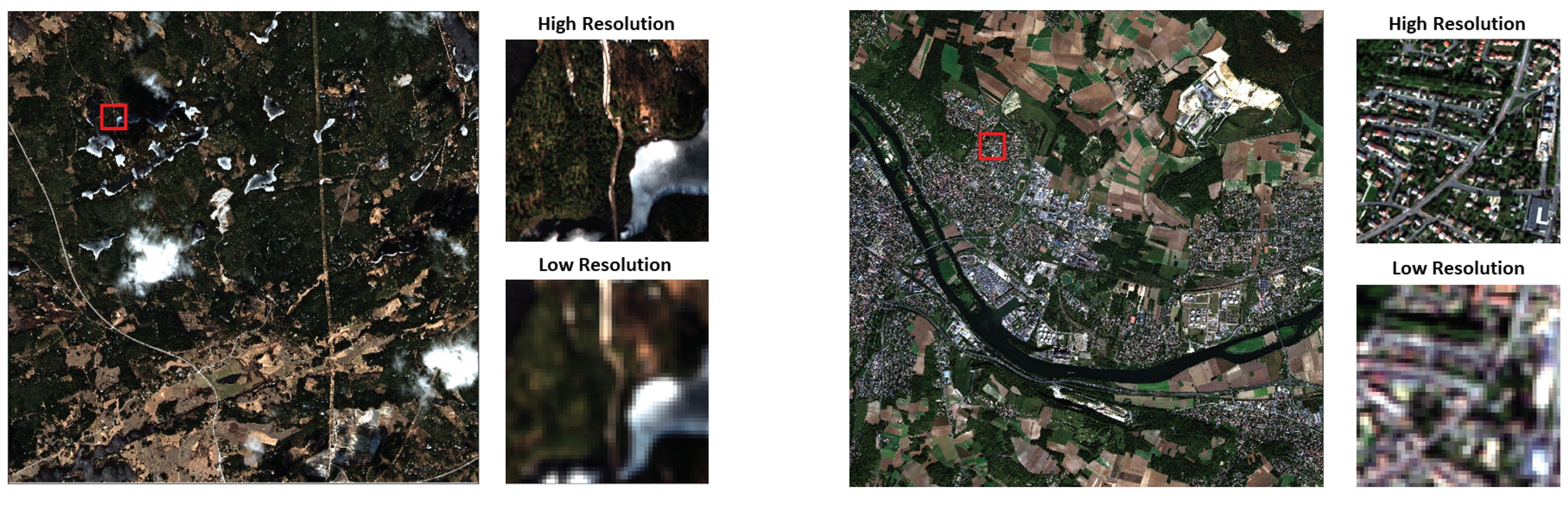
2. Satellite Images

Sentinel-2 is a satellite mission developed within the Copernicus program, a joint initiative of the European Commission, the European Space Agency and the European Environment Agency, to provide operational information of our planet for safety and environmental applications. It is composed of two identical satellites: Sentinel-2A (launched on June 2015) and Sentinel-2B (launched on March 2017) flying in the same orbit but phased at 180° to give a high revisit frequency of 5 days at the Equator. Each satellite carries a multispectral payload (MSI) that provides a set of 13 spectral bands ranging from visible and near infrared (VISNIR) to shortwave infrared (SWIR). In particular, four of these bands (B2, B3, B4 and B8) record data at a spatial resolution of 10 m, six bands at 20 m and three bands at 60 m. Basically, bands at lower resolution are devoted to the analysis of the vegetation status, discrimination of snow, ice and clouds and to retrieve information about aerosols, water-vapor and cirrus. Data is available at [49]

To improve the spatial resolution of the Sentinel-2 10 m bands using super-resolution techniques, multispectral WorldView data was used to produce the LR-HR training dataset. Worldview-2, launched on October 2009, was the first high-resolution 8-band multispectral commercial satellite [50]. Operating in a nearly circular sun-synchronous orbit at an altitude of 770 km, it provides a 1.84 m resolution for the VISNIR multispectral bands and a panchromatic band of 46 cm. WorldView-3 was launched on August, 2014 at an altitude of approximately 617 km, providing 8 multispectral bands at 1.24 m in the VISNIR plus additional shortwave infrared bands at 3.7 m and a panchromatic band of 31 cm.

Table 1. Spatial and spectral characteristics of Sentinel-2 and WorldView-2/3 satellites (visible and near infrared multispectral bands).

Satellite	Spectral Band	Central Wavelenght (nm)	Bandwidth (nm)	Spatial Resolution-GSD (m)
	B1: Coastal Aerosol	443	20	60
	B2: Blue	490	65	10
	B3: Green	560	35	10
	B4: Red	665	30	10
Sentinel-2	B5: Red-edge 1	705	15	20
	B6: Red-edge 2	740	15	20
	B7: Red-edge 3	783	20	20
	B8: Near-IR	842	115	10
	B8A: Near-IR narrow	865	20	20
	B9: Water Vapor	945	20	60
	B1: Coastal Blue	425	47.3	Nadir
	B2: Blue	480	54.3	WV-2: 1.84 m
	B3: Green	545	63.0	WV-3: 1.24 m
WorldView-2/3	B4: Yellow	605	37.4
	B5: Red	660	57.4	20° off Nadir
	B6: Red-edge	725	39.3	WV-2: 2.40 m
	B7: Near-IR 1	833	98.9	WV-3: 1.38 m
	B8: Near-IR 2	950	99.6

lists the technical characteristics of Sentinel-2 and Worldview-2/3 spectral bands in the VISNIR spectrum.

3. Materials and Methods

3.1. Datasets

We used two datasets to train the models, the WorldView European Cities dataset [51] and a collection of pairs of WorldView-Sentinel images. A third dataset of WordView-Sentinel image pairs was used as an independent test set, to evaluate the performance of the model. In the following, we will refer to the two WordView-Sentinel datasets as W-S Set1 and W-S Set2, respectively.

The European Cities dataset is a large collection of publicly available WorldView-2 images provided by the European Space Agency (ESA). These images were sensed by the satellite from July 2010 to July 2015 covering several areas of Europe. Some examples are shown in Figure 1. Care was taken in selecting scenes with little or no cloud cover in the image. We used 32 large images covering part of Ireland, France, the United Kingdom, Malta, Italy, Spain and others areas, aiming to provide a variety of covers like agriculture landscapes, cities, shores, forest areas, etc.

The W-S Set1 used to train the model consisted of pairs of WorldView-Sentinel images that were sensed on the Canary and Balearic Islands in Spain. Images were provided by the ARTEMISAT-2 project [52] and correspond to regions of the Maspalomas Natural Reserve, Teide National Park, and Cabrera archipelago. Sensing dates and the original resolution of the WorldView images can be seen at

Table 2. W-S Set1: WorldView and Sentinel-2 pairs.

Location	Year	Sentinel-2	WorldView-2	WorldView-3	Resolution
	2015	29 September	4 June	-	2.0 m
Maspalomas	2017	10 June	10 June	-	1.6 m
	2017	31 May	-	31 May	1.6 m
Cabrera	2016	5 September	1 September	-	2.0 m
Teide	2017	10 June	-	13 June	1.2 m
	2018	31 May	1 June	-	2.0 m

. The W-S Set2 dataset was composed with pairs of WorldView and Sentinel-2 images that were used to test the robustness of the model to unseen images during training. Details are provided in

Table 3. W-S Set2: WorldView and Sentinel-2 pairs.

Location	Year	Sentinel-2	WorldView-2	WorldView-3	Resolution
Cabrera	2019	10 May	10 May	-	2.0 m
Maspalomas	2018	31 May	-	22 May	1.2 m

.

3.2. Image Pre-Processing

The WorldView ortho-ready standard level 2 product was used in the study as the target data. These standard imagery products are radiometrically corrected (relative radiometric response between detectors, non-responsive detector fill, and a conversion for absolute radiometry), sensor corrected (internal detector geometry, optical distortion, scan distortion and any line-rate variations), geometrically corrected (spacecraft orbit position and attitude uncertainty, Earth rotation and curvature and panoramic distortion) and projected [50].

To obtain true radiance values from the digital values of the image, it was necessary to perform a radiometric calibration applying the correct gains and offsets of the sensor for each band. After this calibration, Top Of Atmosphere (TOA) radiances were obtained. TOA radiance includes distortions produced by the absorption and scattering of the atmospheric gases and, in consequence, correction algorithms are necessary to minimize these effects for the different wavelength of the spectrum.

After a thorough assessment of different advanced atmospheric corrections models, comparing Worldview-2 estimated reflectances with real ones measured by a field spectroradiometer [53], most of the radiative models tested achieved good performance but the Fast Line-of-sight Atmospheric Analysis of Hypercubes (FLAASH) algorithm [54] provided the highest accuracy with Root Mean Square Error (RMSE) values around 3%.

The FLAASH model was applied and the corresponding parameters (atmosphere type, aerosol model and thickness, height, flight time and date, sensor geometry, adjacency, etc.) were properly set using climatic and field data besides the information included in the metadata file of each image. Next, to transform the perspective of a satellite-derived image to an orthogonal view of the ground, which removes the effects of sensor tilt and terrain relief, orthorectification was applied using rational polynomial coefficients and a high-resolution digital elevation model.

On the other hand, the available Sentinel-2 Level-2A products, that already provide Bottom Of Atmosphere (BOA) reflectance images, were considered for the analysis. Specifically, the Level-2A processing protocol mainly includes an atmospheric correction applied to the TOA Level-1C and the orthorectification [2]. The atmospheric correction model used is Sen2Cor [55], which is a combination of state-of-the-art techniques tailored to the Sentinel-2 environment.

Once Worldview and Sentinel images were properly pre-processed, both sets were modified to have the same spatial resolution of 2 m and properly co-registered. The process included locating and matching a number of ground control points (GCP) in both images and then performing a geometric transformation. Automatic and manual GCP were extracted to derive a representative and well distributed set of points. Next, a polynomial warping algorithm was applied to the Sentinel image to match the reference Worldview image [56]. We only considered those channels that overlap each other, specifically bands B2, B3, B4 and B8 of Sentinel-2 and bands B2, B3, B5 and B7 of WorldView as detailed in Table 1.

WorldView images in the European Cities dataset have a GSD of 1.6 m. Corrections were made to obtain the BOA reflectance images as well. To form LR-HR pairs, we used the BOA images as the HR and down-sampled them to obtain the LR image, preserving the same scaling factor as the WorldView-Sentinel pairs, as shown in Figure 2. Then, the LR European Cities images were interpolated using bicubic interpolation. Finally, we selected the same set of bands as for the WorldView-Sentinel dataset.

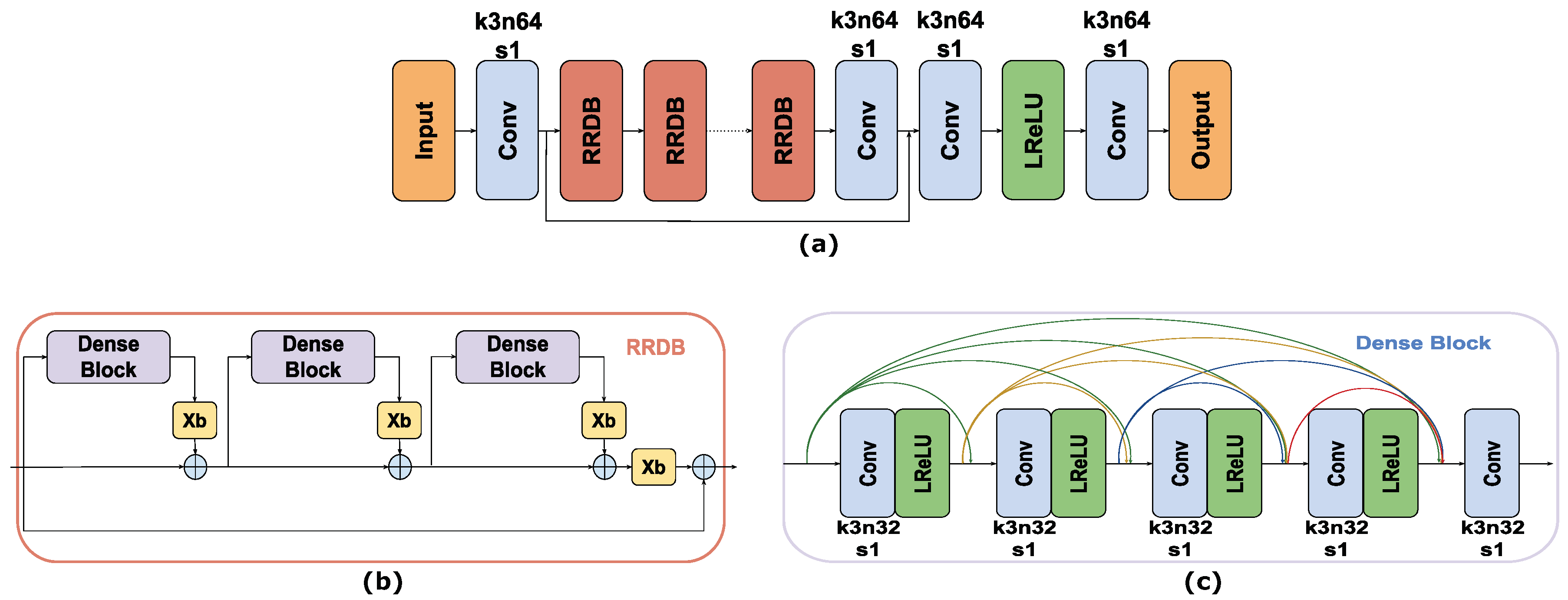
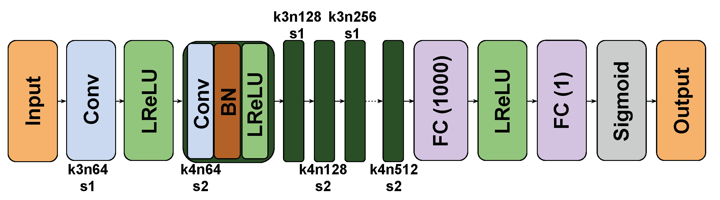
3.3. Network Architecture

Since the work of [35], GANs have been used in super-resolution tasks due to their ability to generate realistic outputs with rich textures and quality. The idea of using two models trained simultaneously was proposed in [34], where a Generator network (G) is trained aiming to produce new data-samples by capturing the data distribution from the training data. At the same time, a Discriminator network (D) is trained aiming to verify the authenticity of the generated samples by evaluating the probability of this data to correspond to the training distribution rather than being generated by G. This training process involves minimizing the error between the generated and real samples on one hand, and maximizing the chances of distinguishing between the real and the generated (fake) samples on the other, making the cost function to depend on both networks, G and D. Figure 3 shows the relationship between the networks, where the Generator has only access to the input data while the Discriminator has access to both, generated and real data [57].

When GANs are used for super-resolution, a generator is trained to produce a realistic version of a HR image from a LR version. In this work we based our model on the Enhanced Super-Resolution Generative Adversarial Network [37] due to its high performance in super-resolution of natural images.

The architecture of the Generator network can be seen in Figure 4 with the corresponding configuration of kernel size (k), feature maps (n) and stride (s) for each convolutional layer. A single convolutional layer is used as a feature extractor to generate 64 feature maps with 3 × 3 kernels with stride 1. These maps are the input of a deeper feature extractor composed by 23 Residual-in-Residual Dense Blocks (RRDB) and, finally, three convolutional layers are used to reconstruct the output. A long range skip-connection transfers low-level features that are combined with high-level features learned by the RRDB.

The residual learning block RRDB has a more dense and complex structure of convolutional layers with 3 × 3 kernels and 32 feature maps. All convolutional layers use stride 1 to maintain the resolution of the images throughout the generator. The nonlinear activation is the leaky-ReLU with a negative slope of 0.2. Each Dense Block allows the propagation of the information learned by preceding layers, increasing the network capacity by using effectively this residual and local information. The concept of Residual Scaling [58] was used to down scale feature maps by factor given by a hyperparameter $X_b$ (see Figure 4b) to prevent instability in training very deep networks.

Since we use an interpolated version of the LR image as an input image (see Section 3.2), the upsampling modules of the original ESRGAN implementation were removed from the Generator. Besides, the input and output layers were adapted to work with the four bands.

Figure 5 shows the architecture of the Discriminator network (D). It contains 8 blocks formed by convolution, batch-normalization and leaky-ReLU layers. The blocks contain an increasing number of feature maps, reaching 512 filters with alternating kernel sizes, a 3 × 3 kernel for a convolutional layer with stride 1, and a 4 × 4 kernel with stride 2 for reducing the size of the images when the number of feature maps is increased. The last layers are two dense fully-connected layers together with a final sigmoid output to produce the final score.

3.4. Methodology and Loss Functions

We train the model in three stages. First, we train the generator using the European Cities dataset, then, in a second stage, we fine tune the generator using image pairs from the W-S Set1. For these two stages, we use the $L_1$ loss (Equation (1)), that measures the mean absolute error between the generated output $G\left(X_i\right)$ and the target $Y_i$ for each ith image.

$$L_1={\mathbb{E}}_{X_i}∥G\left(X_i\right)-Y_i∥$$

(1)

After training the Generator with the European Cities dataset and the WorldView-Sentinel image pairs, the third and final stage consists in training the Generator along with the Discriminator with an adversarial approach, using the weights learned from previous stages, and only training the models with WorldView-Sentinel pairs. In this stage, a combination of losses is used for updating the weights of the Generator (Equation (2)) and the Discriminator (Equation (6)). The Generator loss $L_G$ is a sum of three terms: the adversarial loss $L_G^{Ra}$ (Equation (5)), the content loss $L_1$ (Equation (1)), and the perceptual loss $L_{percep}$ (Equation (3)).

$$L_G=\eta L_1+\lambda L_G^{Ra}+\gamma L_{percep}$$

(2)

The perceptual loss $L_{percep}$, introduced by [36], uses the VGG-19 network [59] as feature extractor, and measures the difference between feature maps obtained in two different points in the network. It computes the mean absolute error between feature maps obtained after the 4th convolutional layer and before the 5th max-pooling layer (${\varphi }_{54}(.)$), for each target image $Y_i$ and output $G\left(X_i\right)$.

$$L_{percep}={\mathbb{E}}_{X_i}∥{\varphi }_{54}\left(G\left(X_i\right)\right)-{\varphi }_{54}\left(Y_i\right)∥$$

(3)

The adversarial loss $L_G^{Ra}$ is calculated taking into account the concept of the Relativistic average GAN (Ra) scheme introduced by Jolicoeur-Martineau in [38]. Relativistic average GAN improves the performance of a standard GAN by encouraging the discriminator to not only distinguish between input real images ($x_r$) and fake images ($x_f$), but instead to distinguish that a real input image is relatively more realistic than a fake one.

A standard GAN computes the probability that the generic input data x is real as $D\left(x\right)=\sigma \left(C\right(x\left)\right)$, where $\sigma (.)$ is the sigmoid function and $C\left(x\right)$ is the non-transformed discriminator output. By using the relativistic scheme, the probability of a real data to be classified as real decreases while increases the probability of fake data being classified as real. The relativistic discriminator ($D_{Ra}$) takes into account a priori knowledge that half of the mini-batch samples are even fake or real. So, the ($D_{Ra}$) is formulated as shown in Equation (4), where ${\mathbb{E}}_{x_f}[.]$ represents the operation of computing the mean of all fake data in the mini-batch [38].

$$D_{Ra}(x_r,x_f)=\sigma (C\left(x_r\right)-{\mathbb{E}}_{x_f}\left[C\left(x_f\right)\right])$$

(4)

Cross-entropy is used to calculate the adversarial loss $L_G^{Ra}$ as shown in Equation (5). Due to the mini-max behavior of GANs, as one of the networks wants to minimize the probability of fake data to be detected and the other wants to increase its probability to discriminate between fake and real data, cross-entropy is used in a symmetrical form to update the weights of the Generator and Discriminator (Equation (6)), since both networks benefit from the information of real and generated data in an adversarial training, making results more realistic and with more details [37].

$$L_G^{Ra}=-{\mathbb{E}}_{x_r}\left[log(1-D_{Ra}(x_r,x_f))\right]-{\mathbb{E}}_{x_f}\left[log\left(D_{Ra}(x_r,x_f)\right)\right]$$

(5)

$$L_D^{Ra}=-{\mathbb{E}}_{x_r}\left[log\left(D_{Ra}(x_r,x_f)\right)\right]-{\mathbb{E}}_{x_f}\left[log(1-D_{Ra}(x_r,x_f))\right]$$

(6)

3.5. Training Details and Network Interpolation

Due to the large size of satellite images, around 10 K × 10 K pixels in European Cities dataset and over 1 K × 1 K in the WorldView-Sentinel dataset, images were divided into tiles of 140 × 140 pixels to form the train-validation-test subsets. The European Cities dataset contains 32 large images of different parts of Europe, that were tiled and used for pre-training the model. The WorldView-Sentinel dataset W-S Set1 contains 5293 tiles for training, 278 for validation and 296 for test. We performed horizontal and vertical flips for data augmentation as well as random crops of 128 × 128 pixels. Adam optimization [60] was used, with an initial learning rate of 10${}^{-4}$, halved every 20K iterations. The hyperparameters that weight the different losses in Equation (2) are $\eta ={10}^{-2}$, $\gamma =1$ and $\lambda =5^{-3}$ as in [37]. The batch size is 2 and the residual scaling parameter is $X_b=0.2$.

As indicated, the networks were trained in three stages, first with images from the European Cities dataset, then using the WorldView-Sentinel (W-S) Set1 for training the generator network alone and finally fine-tuning the model with adversarial training and using the same W-S Set1. We have used Pytorch framework training the models with a Nvidia GTX Titan X 12GB and 12GB of RAM memory, taking each stage 21 h to be completed.

The final SR image from a LR image X is obtained as a linear combination between a generator trained in adversarial mode $G_{adv}\left(X\right)$ and a generator trained alone $G_{PSNR-oriented}\left(X\right)$ (Equation (7)). This linear combination is done to remove unpleasant noise produced by purely GAN-based methods while maintaining a good perceptual quality [37]. The interpolation parameter $\alpha$ is a real number within the $[0,1]$ range.

$$G\left(X\right)=(1-\alpha )G_{PSNR-oriented}\left(X\right)+\alpha G_{adv}\left(X\right)$$

(7)

3.6. Quality Assessment

To perform a quantitative comparison of the results obtained by the Generator ($G\left(X\right)$) using the input LR image (X) from the test set, and compared to its target HR image (Y), several metrics were considered.

• Peak Signal to Noise Ratio (PSNR): it is one of the standard metrics used to evaluate the quality of a reconstructed image. Here, MaxVal is the maximum value of the HR image (Y). Higher PSNR generally indicates higher image quality.

  $$PSNR(G\left(X\right),Y)=20lo{g}_{10}\left(\frac{MaxVal}{RMSE\left[G\right(X),Y]}\right)$$

  (8)
• Structural Similarity (SSIM) [61]: it is a metric that measures the similarity between two images taking into account three aspects: luminance, contrast and structure. It is in the range $[-1,1]$, where a SSIM equal to 1 corresponds to identical images. Constants $C_1=k_{1}L$ and $C_2=k_{2}L$ are values that depends on the dynamic range (L) of the pixels values, with $k1=0.01$ and $k2=0.03$ by default.

  $$SSIM(G\left(X\right),Y)=\frac{(2{\mu }_X{\mu }_Y+C_1)(2{\sigma }_{XY}+C_2)}{({\mu }_X^2+{\mu }_Y^2+C_1)({\sigma }_X^2+{\sigma }_Y^2+C_2)}$$

  (9)
• Erreur relative globale adimensionnelle de systhese (ERGAS) [62]: it measures the quality of the output $G\left(X\right)$ image by taking into consideration the scaling factor (S) as well as the normalized error per channel, considering the mean ${\overline{Y}}_j$ of each band. Contrary to the PSNR and SSIM metrics for this index a lower value implies higher quality.

  $$ERGAS(G\left(X\right),Y)=100S\sqrt{\frac{1}{n_{bands}}\sum _{j=1}^{n_{bands}}{\left[\frac{RMSE(G{\left(X\right)}_j,Y_j)}{{\overline{Y}}_j}\right]}^2}$$

  (10)
• Spectral Angle Mapper (SAM) [63]: it calculates the angle between two images by computing the dot product divided by the 2-norm of each image. This index indicates higher similarity between images as it approaches zero.

  $$SAM(G\left(X\right),Y)=arccos\left(\frac{G\left(X\right).Y}{{∥G\left(X\right)∥}_2{∥Y∥}_2}\right)$$

  (11)
• Correlation Coefficient (CC): it computes the linear correlation between the images. It is in the range $[-1,1]$, where 1 is total positive linear correlation and n is the number of pixel in each channel.

  $$CC(G\left(X\right),Y)=\frac{1}{n_{bands}}\sum _{j=1}^{n_{bands}}\left\{\frac{{\sum }_{k=0}^n(G{\left(X\right)}_{kj}-{\overline{G\left(X\right)}}_j)(Y_{kj}-{\overline{Y}}_j)}{\sqrt{{\sum }_{k=0}^n{[G{\left(X\right)}_{kj}-{\overline{G\left(X\right)}}_j]}^2}\sqrt{{\sum }_{k=0}^n{[Y_{kj}-{\overline{Y}}_j]}^2}}\right\}$$

  (12)

For a qualitative comparison, true RGB and false-color composites were used to evaluate the overall spatial and spectral performance of the methods. The false-color image is composed of the NIR, Red and Green channels, in that order.

4. Experiments and Results

In this section we present numerical and visual results of our model applied to the test subset of the W-S Set1, for several values of the interpolation parameter $\alpha$ (Equation (7)). Next, we evaluate the robustness of the model on an independent set of images using W-S Set2. Finally, a comparison with other state-of-the-art super-resolution algorithms is presented. In all cases quantitative results are given in terms of mean and standard deviation of the quality metrics on the test sets. In addition, statistical tests were performed to analyse the statistical significance of the difference in performance of our method and other state-of-the-art models.

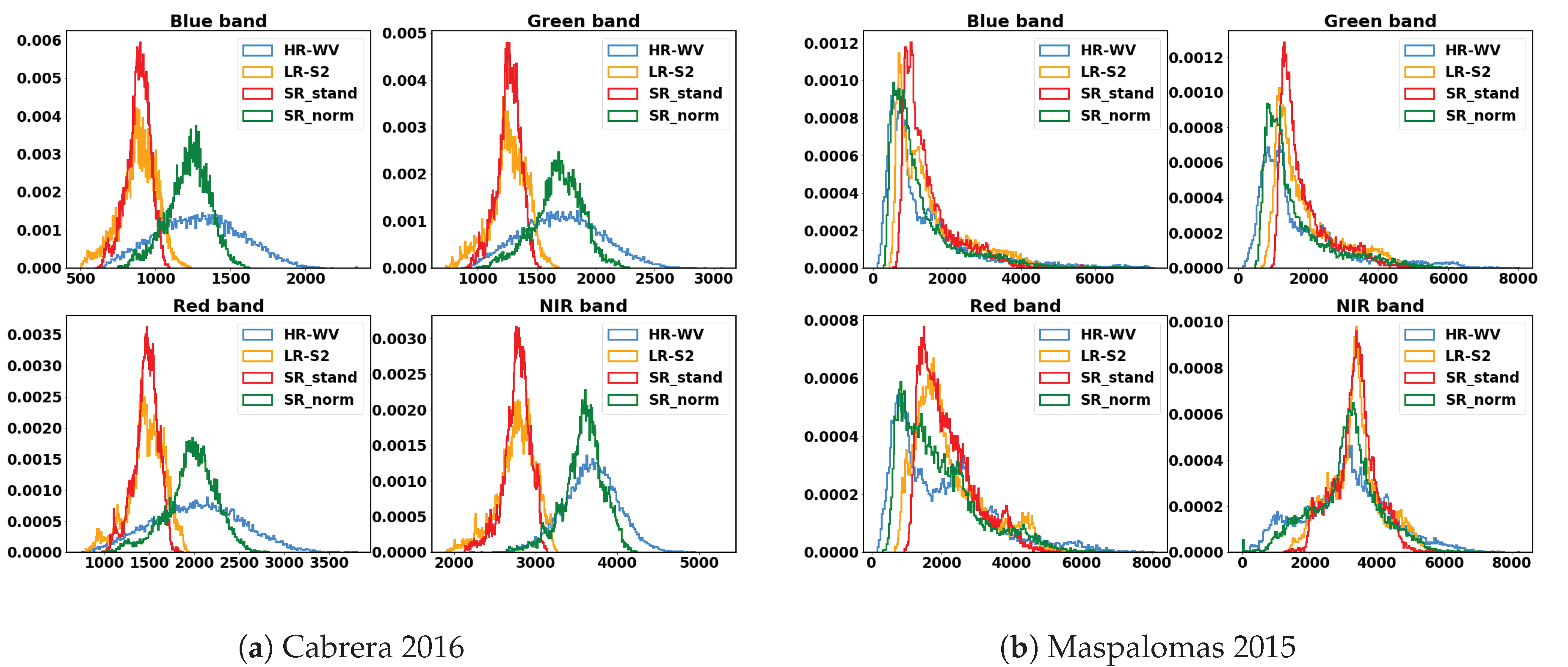
4.1. Data Standardization

Data normalization is typically performed prior to training a neural network to speed up learning and lead to faster convergence. The usual approach in SR models consists in dividing all image pixels by the largest pixel value, adjusting pixel values to the [0,1] range. This is performed across all channels, regardless of the actual range of pixel values that are present in the image. The inverse process is done at the output, re-scaling pixels to the original range.

However, we have observed that this type of normalization does not perform well in our scheme that is trained with images from two different sensors, leading to results where the distribution of the SR Sentinel image is shifted towards the spectral distribution of the original WorldView HR image.

To address this issue, we standardize the input and target data. Standardization is done by channel j, subtracting the mean $\overline{X_j}$ and dividing by the standard deviation ${\sigma }_{X_j}$. To obtain the final SR image $G\left(X\right)$, the inverse process is applied, using the mean and standard deviation of the input image X, as shown in Equations (13) and (14).

$$\widehat{X_j}=\frac{X_j-\overline{X_j}}{{\sigma }_{X_j}}$$

(13)

$$G\left(X_j\right)=G\left(\widehat{X_j}\right){\sigma }_{X_j}+\overline{X_j}$$

(14)

Figure 6 illustrates the difference between the two methods. We have trained both models, one normalizing and the other one standardizing the data, and we generated SR results for two samples from the W-S Set1 corresponding to Cabrera and Maspalomas. We present the normalized histograms per band. Each plot shows the original distribution of the LR Sentinel (orange), HR WordView (blue), the SR output using normalization (green) and standardization (red). We clearly observe that the standardization approach helps to preserve the spectral content of the low resolution image.

4.2. Performance on the W-S Set1

Table 4. Quality metrics results on the W-S Set1 for nearest neighbor (LR_nn) and bicubic (LR_cub) interpolation and our method SR_$\alpha$ for different values of $\alpha$.

		LR_nn	LR_cub	SR_0	SR_0.1	SR_0.2	SR_0.5	SR_0.7	SR_1
PSNR	mean	26.048	26.049	28.099	28.036	27.893	27.476	27.160	26.099
	std	2.368	2.368	2.249	2.287	2.326	2.369	2.357	2.323
SSIM	mean	0.527	0.527	0.622	0.624	0.621	0.605	0.585	0.514
	std	0.103	0.103	0.093	0.092	0.093	0.093	0.094	0.096
ERGAS	mean	26.504	26.502	25.389	25.386	25.463	25.75	25.943	26.440
	std	9.072	9.071	8.359	8.319	8.327	8.435	8.496	8.847
SAM	mean	0.121	0.121	0.095	0.096	0.098	0.103	0.107	0.121
	std	0.054	0.054	0.041	0.042	0.043	0.047	0.049	0.055
CC	mean	0.934	0.934	0.959	0.958	0.956	0.951	0.948	0.934
	std	0.053	0.053	0.032	0.033	0.035	0.04	0.042	0.052

shows the quantitative assessment results of our SR model for several values of the interpolation parameter $\alpha$ (Equation (7)), as well as baseline results obtained using nearest neighbor (LR_nn) and bicubic (LR_cub) interpolations of the LR images. The best results are highlighted in bold. Better metrics are obtained for low values of $\alpha$, achieving an improvement over bicubic interpolation of 2.05 dB on PSNR, 0.097 on SSIM, a decrease of 1.116 on ERGAS, a decrease of 0.026 on SAM and an improvement of 0.025 on CC. Figure 7, Figure 8, Figure 9 and Figure 10 provide visual results for several values of $\alpha$ and different land covers. It can be observed that as the influence of the network with adversarial training increases (with $\alpha >0.5$) more texture appears in the SR image. This behaviour is helpful in regions with small details like forest and urban areas, though lower metrics are obtained as a trade-off. However, very large values of $\alpha$ may introduce some artifacts. This is consistent with the typical hallucination effect that has been reported in GAN models [35,37]. It is important to emphasize that only the Sentinel LR image is applied to the trained model and the Worldview HR image is just used as a reference to assess the quality.

4.3. Performance on the W-S Set2

We also tested our model on pairs of WorldView-Sentinel images that were not used for the training, the W-S Set2. Quantitative results are summarized in

Table 5. Quality metrics results on the W-S Set2 for nearest neighbor (LR_nn) and bicubic (LR_cub) interpolation and our method SR_$\alpha$ for different values of $\alpha$.

		LR_nn	LR_cub	SR_0	SR_0.1	SR_0.2	SR_0.5	SR_0.7	SR_1
PSNR	mean	26.280	26.30	27.851	27.912	27.848	27.455	27.085	26.019
	std	1.617	1.657	1.498	1.530	1.572	1.612	1.616	1.605
SSIM	mean	0.588	0.589	0.673	0.676	0.675	0.661	0.644	0.579
	std	0.075	0.077	0.062	0.061	0.061	0.063	0.065	0.070
ERGAS	mean	29.773	29.795	29.909	29.810	29.830	29.726	29.673	29.301
	std	9.072	9.071	8.359	8.319	8.327	8.435	8.496	8.847
SAM	mean	0.176	0.175	0.147	0.146	0.147	0.154	0.161	0.183
	std	0.041	0.040	0.033	0.034	0.036	0.039	0.041	0.047
CC	mean	0.929	0.929	0.950	0.951	0.950	0.945	0.939	0.922
	std	0.053	0.052	0.036	0.036	0.037	0.042	0.046	0.059

.

The proposed model outperforms nearest-neighbor and bicubic interpolation in all the metrics considered. In line with the results achieved with the W-S Set1, low values of $\alpha$ provide, in general, better quality metrics. In this experiment, $\alpha =0.1$ is the optimal value with improvements of 1.612 dB on PSNR and 0.087 on SSIM over bicubic interpolation.

Visual results are presented in Figure 11 and Figure 12 for two images of Maspalomas and Cabrera. It can be inferred from these results a good recovery of the textures in dense forest areas. For images with high density of households, objects are clearly defined, recovering the delimitation of roads and roundabouts. Moreover, there is good spectral agreement between LR images and the SR results, despite of using test images not belonging to the training set.

In accordance with the results of the previous experiments, as we get more influence from the adversarial network (with higher values of $\alpha$), more spatial details appear in the results, at the expense of a slight spectral distortion measured by the quality metrics.

4.4. Comparison with Other SR Models

In this subsection we compare the performance of our proposed RS-ESRGAN model (using $\alpha =0$) with the baseline bicubic interpolation and some state-of-the-art SR methods: SRCNN [64], EDSR [65], RCAN [66] and SRGAN [35].

For a fair comparison, all SR models considered were trained in the same way in two stages, first with European-Cities and then with WorldView-Sentinel Set1, with training details as described in Section 3.5. The upsampling modules of the EDSR, RCAN and SRGAN were removed from the original architectures and input images were pre-upsampled by a factor of 5 using bicubic interpolation. In addition, the architectures of were adapted to work with the four input channels considered. Quality metrics results on the W-S Set1 are summarized in

Table 6. Quality metrics results on W-S Set1 for different methods.

		LR_cub	SRCNN [64]	EDSR [65]	RCAN [66]	SRGAN [35]	RS-ESRGAN (α = 0)	RS-ESRGAN (α = 0.5)
PSNR	mean	26.049	26.528	26.481	27.029	26.898	28.099	27.476
	std	2.368	2.315	2.337	2.269	2.248	2.249	2.369
SSIM	mean	0.527	0.586	0.600	0.617	0.602	0.622	0.605
	std	0.102	0.092	0.094	0.092	0.091	0.093	0.093
ERGAS	mean	26.503	26.746	26.421	26.401	26.717	25.389	25.750
	std	9.072	9.070	8.758	8.579	9.021	8.359	8.435
SAM	mean	0.121	0.115	0.115	0.107	0.110	0.0954	0.103
	std	0.053	0.051	0.045	0.042	0.046	0.040	0.047
CC	mean	0.934	0.942	0.942	0.949	0.947	0.958	0.951
	std	0.053	0.046	0.039	0.034	0.039	0.031	0.040

. The best results are highlighted in bold.

Our model outperforms the others in all the metrics considered. The statistical analysis of the results on the W-S Set1 shows that differences between the proposed model and the other SR models are significant (all p-values smaller than $0.01$).

In addition to the quantitative comparisons, we also performed visual comparisons among our method and the above-listed methods, presented in Figure 13 and Figure 14. The proposed model with $\alpha =0$ and $\alpha =0.1$ produces a clean image, with fine details, less artifacts and consistent with the target.

5. Discussion

Single-Image SR with GANs is a complex task requiring a great quantity of diverse image pairs for training. In addition, in the remote sensing context, the pre-processing steps applied to the data play a key role during the network training.

Aiming to exploit the open policy of Sentinel-2 and the very high spatial resolution that a WorldView imagery offers, we trained our model with real data from both satellite sensors. However, the generation of LR-HR image pairs is not easy mainly due to the high cost and availability of archived data for WorldView, as well as the difficulty of obtaining pairs of similar dates and lighting conditions. To alleviate this inconveniences, the network was pre-trained using LR-HR image pairs artificially generated from a collection of publicly available WorldView images.

One crucial pre-processing step is co-registration, necessary to compensate the miss-alignment of pixels between both datasets. The ability of WorldView to record images with different off-nadir angles may add spatial distortions in comparison with Sentinel imagery, that only senses in the nadir viewing direction, making more complex the generation of LR-HR pairs and requiring the application of orthorectification tasks with a precise digital elevation model. To perform an accurate co-registration, images must have the same GSD to define the ground control points and to apply the subsequent geometric transformation. We performed a bicubic interpolation on the LR images followed by the co-registration. Thus, the upsampled versions of the LR images were input to the network and we removed the upsampling module that is typically used in super-resolution networks like the ESRGAN.

Another important aspect to consider during the generation of LR-HR image pairs is the spectral information, particularly when dealing with sensors having bands with different spectral range. We used the four bands (RGB-NIR) that presented spectral overlap between both satellites. We observed that the standardization of the input and target images before the training was critical to produce SR images preserving the spectral information from the LR counterpart.

The proposed RS-ESRGAN model achieves a significant improvement in all the quality metrics compared to recent models like RCAN and SRGAN. Also, the subjective evaluation shows that the proposed RS-ESRGAN produces finer details and textures. The false color scheme, using the NIR band, shows that improvements are consistent in the four channels considered.

The final SR image is obtained as a linear combination of the results produced by the model trained with and without the adversarial scheme. The interpolation parameter $\alpha$ controls the trade-off between images with high-frequency details and texture, and higher visual quality in general (but also possible artifacts), or images without noise but with less spatial details producing higher quantitative metrics.

The performance on the independent test set W-S Set2 was also excellent. The model was trained with samples containing several structures like building, roads, shrubbery, arid zones and dense vegetation areas and, therefore, can generalize to images from geographical areas that are not included in the training sets. Actually, RS-ESRGAN was also tested with Sentinel-2 images from other parts of the world with satisfactory visual results. To avoid extending this article further, such additional results are not included.

The proposed single-image SR model produces HR images that can enable the use of Sentinel-2 imagery in several studies where fine detail is needed. Moreover, the user can decide about exploiting the spatial detail or preserving the spectral agreement by just tuning the interpolation parameter $\alpha$.

The improvement in spatial quality at the expense of generating some noise in the SR image, and the computational burden due to the combination of different loss functions and the dense combination of feature maps in the generator might be a limitation of the model. These issues are currently unsolved and are certainly good topics to be explored in a near future.

Another issue that deserves attention is the presence of artifacts in SR images, that tend to appear with the fully adversarial mode, i.e. with higher values of $\alpha$. Artifacts make roads appear more sinuous when they should be straight or produce the hallucination of connected dense vegetation areas, when HR images demonstrate the opposite. These are important problems to tackle in future works, although network interpolation seems to be a valid workaround in obtaining a SR image less blurry and with texture recovered.

6. Conclusions

In this paper we propose a single-image super-resolution method based on a deep generative adversarial network to enhance the spatial resolution of Sentinel-2 10 m bands to a resolution of 2 m. The proposed model, RS-ESRGAN, was adapted to work with co-registered remote sensing images and it was trained using the four channels (RGB and NIR) that overlap on both satellites, with Sentinel-2 images as input and WorldView images as target. Several pre-processing steps were needed to obtain the dataset of image pairs ready for training. The model was first trained with synthetic LR-HR pairs from the WorldView European Cities dataset and, next, with real LR-HR image pairs from Sentinel-2 and WorldView satellites. An important aspect for the training was the standardization of the images by channels, that proved to be a crucial step to preserve the spectral information between the low-resolution and the super-resolved images. The behaviour of the $\alpha$ parameter was analyzed, showing the trade-off between visual quality and quantitative metrics of the results. Finally, results show significant improvements, both quantitative and qualitatively, of RS-ESRGAN compared to other state-of-the-art deep learning SR models.

References

- WorldView-3 Datasheet. Digital Globe. Available online: http://content.satimagingcorp.com.s3.amazonaws.com/media/pdf/WorldView-3-PDF-Download.pdf. (accessed on 26 June 2020).
- Sentinel-2 User Handbook, ESA Standard Document, Issue I, Rev. 2. Available online: https://earth.esa.int/documents/247904/685211/Sentinel-2_User_Handbook (accessed on 11 December 2019).
- Kpalma, K.; Chikr El-Mezouar, M.; Taleb, N. Recent Trends in Satellite Image Pan-sharpening techniques. In Proceedings of the 1st International Conference on Electrical, Electronic and Computing Engineering, Vrnjacka Banja, Serbia, 2–5 June 2014. [Google Scholar]
- Vivone, G.; Alparone, L.; Chanussot, J.; Dalla Mura, M.; Garzelli, A.; Licciardi, G.A.; Restaino, R.; Wald, L. A critical comparison among pansharpening algorithms. IEEE Trans. Geosci. Remote Sens. 2014, 53, 2565–2586. [Google Scholar] [CrossRef]
- Loncan, L.; De Almeida, L.B.; Bioucas-Dias, J.M.; Briottet, X.; Chanussot, J.; Dobigeon, N.; Fabre, S.; Liao, W.; Licciardi, G.A.; Simoes, M.; et al. Hyperspectral pansharpening: A review. IEEE Geosci. Remote Sens. Magaz. 2015, 3, 27–46. [Google Scholar] [CrossRef]
- Mookambiga, A.; Gomathi, V. Comprehensive review on fusion techniques for spatial information enhancement in hyperspectral imagery. Multidimens. Syst. Signal Proces. 2016, 27, 863–889. [Google Scholar] [CrossRef]
- Yokoya, N.; Grohnfeldt, C.; Chanussot, J. Hyperspectral and multispectral data fusion: A comparative review of the recent literature. IEEE Geosci. Remote Sens. Magaz. 2017, 5, 29–56. [Google Scholar] [CrossRef]
- Garzelli, A.; Aiazzi, B.; Baronti, S.; Selva, M.; Alparone, L. Hyperspectral image fusion. In Proceedings of the Hyperspectral Workshop, Frascati, Italy, 17–19 March 2010. [Google Scholar]
- Dian, R.; Li, S.; Fang, L.; Wei, Q. Multispectral and hyperspectral image fusion with spatial-spectral sparse representation. Inform. Fusion 2019, 49, 262–270. [Google Scholar] [CrossRef]
- Marcello, J.; Ibarrola-Ulzurrun, E.; Gonzalo-Martín, C.; Chanussot, J.; Vivone, G. Assessment of Hyperspectral Sharpening Methods for the Monitoring of Natural Areas Using Multiplatform Remote Sensing Imagery. IEEE Trans. Geosci. Remote Sens. 2019, 57, 8208–8222. [Google Scholar] [CrossRef]
- Huang, W.; Xiao, L.; Wei, Z.; Liu, H.; Tang, S. A new pan-sharpening method with deep neural networks. IEEE Geosci. Remote Sens. Lett. 2015, 12, 1037–1041. [Google Scholar] [CrossRef]
- Masi, G.; Cozzolino, D.; Verdoliva, L.; Scarpa, G. Pansharpening by convolutional neural networks. Remote Sens. 2016, 8, 594. [Google Scholar] [CrossRef]
- Palsson, F.; Sveinsson, J.R.; Ulfarsson, M.O. Multispectral and hyperspectral image fusion using a 3-D-convolutional neural network. IEEE Geosci. Remote Sens. Lett. 2017, 14, 639–643. [Google Scholar] [CrossRef]
- Yang, J.; Fu, X.; Hu, Y.; Huang, Y.; Ding, X.; Paisley, J. PanNet: A deep network architecture for pan-sharpening. In Proceedings of the IEEE International Conference on Computer Vision, Venice, Italy, 22–29 October 2017; pp. 5449–5457. [Google Scholar]
- Yang, J.; Zhao, Y.Q.; Chan, J. Hyperspectral and multispectral image fusion via deep two-branches convolutional neural network. Remote Sens. 2018, 10, 800. [Google Scholar] [CrossRef]
- Scarpa, G.; Vitale, S.; Cozzolino, D. Target-adaptive CNN-based pansharpening. IEEE Trans. Geosci. Remote Sens. 2018, 56, 5443–5457. [Google Scholar] [CrossRef]
- Garzelli, A. A review of image fusion algorithms based on the super-resolution paradigm. Remote Sens. 2016, 8, 797. [Google Scholar] [CrossRef]
- Molini, A.B.; Valsesia, D.; Fracastoro, G.; Magli, E. DeepSUM: Deep neural network for Super-resolution of Unregistered Multitemporal images. IEEE Trans. Geosci. Remote Sens. 2019. [Google Scholar] [CrossRef]
- Haut, J.M.; Fernandez-Beltran, R.; Paoletti, M.E.; Plaza, J.; Plaza, A.; Pla, F. A new deep generative network for unsupervised remote sensing single-image super-resolution. IEEE Trans. Geosci. Remote. Sens. 2018, 56, 6792–6810. [Google Scholar] [CrossRef]
- Wang, P.; Zhang, H.; Zhou, F.; Jiang, Z. Unsupervised remote sensing image super-resolution using cycle CNN. In Proceedings of the IGARSS 2019 IEEE International Geoscience and Remote Sensing Symposium, Yokohama, Japan, 28 July–2 August 2019; pp. 3117–3120. [Google Scholar]
- Yang, J.; Wright, J.; Huang, T.; Ma, Y. Image super-resolution as sparse representation of raw image patches. In Proceedings of the 2008 IEEE Conference on Computer Vision and Pattern Recognition, Anchorage, AK, USA, 23–28 June 2008; pp. 1–8. [Google Scholar]
- Yang, J.; Wright, J.; Huang, T.S.; Ma, Y. Image super-resolution via sparse representation. IEEE Trans. Image Proces. 2010, 19, 2861–2873. [Google Scholar] [CrossRef]
- Dong, W.; Zhang, L.; Shi, G.; Wu, X. Image deblurring and super-resolution by adaptive sparse domain selection and adaptive regularization. IEEE Trans. Image Proces. 2011, 20, 1838–1857. [Google Scholar] [CrossRef]
- Gou, S.; Liu, S.; Yang, S.; Jiao, L. Remote sensing image super-resolution reconstruction based on nonlocal pairwise dictionaries and double regularization. IEEE J. Sel. Top. Appl. Earth Observ. Remote Sens. 2014, 7, 4784–4792. [Google Scholar] [CrossRef]
- Pan, Z.; Yu, J.; Huang, H.; Hu, S.; Zhang, A.; Ma, H.; Sun, W. Super-resolution based on compressive sensing and structural self-similarity for remote sensing images. IEEE Trans. Geosci. Remote Sens. 2013, 51, 4864–4876. [Google Scholar] [CrossRef]
- Zhang, Y.; Du, Y.; Ling, F.; Fang, S.; Li, X. Example-based super-resolution land cover mapping using support vector regression. IEEE J. Sel. Top. Appl. Earth Observ. Remote Sens. 2014, 7, 1271–1283. [Google Scholar] [CrossRef]
- Li, J.; Yuan, Q.; Shen, H.; Meng, X.; Zhang, L. Hyperspectral image super-resolution by spectral mixture analysis and spatial–spectral group sparsity. IEEE Geosci. Remote Sens. Lett. 2016, 13, 1250–1254. [Google Scholar] [CrossRef]
- Wang, Z.; Chen, J.; Hoi, S.C. Deep learning for image super-resolution: A survey. arXiv 2019, arXiv:1902.06068. [Google Scholar] [CrossRef] [PubMed]
- Dong, C.; Loy, C.C.; He, K.; Tang, X. Learning a deep convolutional network for image super-resolution. In European Conference on Computer Vision; Springer: Berlin/Heidelberg, Germany, 2014; pp. 184–199. [Google Scholar]
- Kim, J.; Kwon Lee, J.; Mu Lee, K. Accurate image super-resolution using very deep convolutional networks. In Proceedings of the IEEE Conference on Computer Vision and Pattern Recognition, Las Vegas, NV, USA, 27–30 June 2016; pp. 1646–1654. [Google Scholar]
- Kim, J.; Kwon Lee, J.; Mu Lee, K. Deeply-recursive convolutional network for image super-resolution. In Proceedings of the IEEE Conference on Computer Vision and Pattern Recognition, Las Vegas, NV, USA, 27–30 June 2016; pp. 1637–1645. [Google Scholar]
- Dong, C.; Loy, C.C.; Tang, X. Accelerating the super-resolution convolutional neural network. In European Conference on Computer Vision; Springer: Berlin/Heidelberg, Germany, 2016; pp. 391–407. [Google Scholar]
- Dong, C.; Loy, C.C.; He, K.; Tang, X. Image super-resolution using deep convolutional networks. In IEEE Transactions on Pattern Analysis and Machine Intelligence; IEEE: Piscataway, NJ, USA, 1 February 2016; Volume 38, pp. 295–307. [Google Scholar]
- Goodfellow, I.; Pouget-Abadie, J.; Mirza, M.; Xu, B.; Warde-Farley, D.; Ozair, S.; Courville, A.; Bengio, Y. Generative adversarial nets. Adv. Neural Inform. Proces. Syst. 2014, 2672–2680. [Google Scholar]
- Ledig, C.; Theis, L.; Huszár, F.; Caballero, J.; Cunningham, A.; Acosta, A.; Aitken, A.; Tejani, A.; Totz, J.; Wang, Z.; et al. Photo-realistic single image super-resolution using a generative adversarial network. In Proceedings of the IEEE Conference on Computer Vision and pattern Recognition, Honolulu, HI, USA, 21–26 July 2017; pp. 4681–4690. [Google Scholar]
- Johnson, J.; Alahi, A.; Fei-Fei, L. Perceptual losses for real-time style transfer and super-resolution. In European Conference on Computer Vision; Springer: Berlin/Heidelberg, Germany, 2016; pp. 694–711. [Google Scholar]
- Wang, X.; Yu, K.; Wu, S.; Gu, J.; Liu, Y.; Dong, C.; Qiao, Y.; Change Loy, C. Esrgan: Enhanced super-resolution generative adversarial networks. In Proceedings of the European Conference on Computer Vision (ECCV), Munich, Germany, 8–14 September 2018. [Google Scholar]
- Jolicoeur-Martineau, A. The relativistic discriminator: a key element missing from standard GAN. arXiv 2018, arXiv:1807.00734. [Google Scholar]
- Ma, W.; Pan, Z.; Guo, J.; Lei, B. Super-resolution of remote sensing images based on transferred generative adversarial network. In Proceedings of the IGARSS 2018-2018 IEEE International Geoscience and Remote Sensing Symposium, Valencia, Spain, 22–27 July 2018; pp. 1148–1151. [Google Scholar]
- Haut, J.M.; Paoletti, M.E.; Fernandez-Beltran, R.; Plaza, J.; Plaza, A.; Li, J. Remote Sensing Single-Image Superresolution Based on a Deep Compendium Model. IEEE Geosci. Remote Sens. Lett. 2019, 16, 1432–1436. [Google Scholar] [CrossRef]
- Haut, J.M.; Fernandez-Beltran, R.; Paoletti, M.E.; Plaza, J.; Plaza, A. Remote Sensing Image Superresolution Using Deep Residual Channel Attention. IEEE Trans. Geosci. Remote Sens. 2019, 57, 9277–9289. [Google Scholar] [CrossRef]
- Lei, S.; Shi, Z.; Zou, Z. Super-resolution for remote sensing images via local–global combined network. IEEE Geosci. Remote Sens. Lett. 2017, 14, 1243–1247. [Google Scholar] [CrossRef]
- Bulat, A.; Yang, J.; Tzimiropoulos, G. To learn image super-resolution, use a gan to learn how to do image degradation first. In Proceedings of the European Conference on Computer Vision (ECCV), Munich, Germany, 8–14 September 2018; pp. 185–200. [Google Scholar]
- Ma, W.; Pan, Z.; Yuan, F.; Lei, B. Super-Resolution of Remote Sensing Images via a Dense Residual Generative Adversarial Network. Remote Sens. 2019, 11, 2578. [Google Scholar] [CrossRef]
- Pouliot, D.; Latifovic, R.; Pasher, J.; Duffe, J. Landsat super-resolution enhancement using convolution neural networks and Sentinel-2 for training. Remote Sens. 2018, 10, 394. [Google Scholar] [CrossRef]
- Beaulieu, M.; Foucher, S.; Haberman, D.; Stewart, C. Deep Image-To-Image Transfer Applied to Resolution Enhancement of Sentinel-2 Images. In Proceedings of the IGARSS 2018-2018 IEEE International Geoscience and Remote Sensing Symposium, Valencia, Spain, 22–27 July 2018; pp. 2611–2614. [Google Scholar]
- Salgueiro, L.; Marcello, J.; Vilaplana, V. Comparative study of upsampling methods for super-resolution in remote sensing. In Proceedings of the International Conference on Machine Vision, Amsterdam, The Netherlands, 16–18 November 2019. [Google Scholar]
- Chen, H.; Zhang, X.; Liu, Y.; Zeng, Q. Generative Adversarial Networks Capabilities for Super-Resolution Reconstruction of Weather Radar Echo Images. Atmosphere 2019, 10, 555. [Google Scholar] [CrossRef]
- Copernicus Open Access Hub. European Space Agency. Available online: https://scihub.copernicus.eu/dhus/#/home. (accessed on 29 June 29 2020).
- Digital Globe Core Imagery Products Guide. Available online: https://www.geosoluciones.cl/documentos/worldview/DigitalGlobe-Core-Imagery-Products-Guide.pdf (accessed on 11 December 2019).
- WorldView-2 European Cities. European Space Agency (ESA). Available online: https://earth.esa.int/web/guest/-/worldview-2-european-cities-dataset (accessed on 22 July 2019).
- Marcello, J. Procesado Avanzado de Datos de Teledetección para la Monitorización y Gestión Sostenible de Recursos Marinos y Terrestres en Ecosistemas Vulnerables—Artemisat2. Available online: http://artemisat2.ulpgc.es/?page_id=35 (accessed on 11 December 2019).
- Marcello, J.; Eugenio, F.; Perdomo, U.; Medina, A. Assessment of atmospheric algorithms to retrieve vegetation in natural protected areas using multispectral high resolution imagery. Sensors 2016, 16, 1624. [Google Scholar] [CrossRef]
- Cooley, T.; Anderson, G.P.; Felde, G.W.; Hoke, M.L.; Ratkowski, A.J.; Chetwynd, J.H.; Gardner, J.A.; Adler-Golden, S.M.; Matthew, M.W.; Berk, A.; et al. FLAASH, a MODTRAN4-based atmospheric correction algorithm, its application and validation. In Proceedings of the IEEE International Geoscience and Remote Sensing Symposium, Toronto, ON, Canada, 24–28 June 2002; Volume 3, pp. 1414–1418. [Google Scholar] [CrossRef]
- Main-Knorn, M.; Pflug, B.; Louis, J.; Debaecker, V.; Müller-Wilm, U.; Gascon, F. Sen2Cor for Sentinel-2. Image and Signal Processing for Remote Sensing XXIII. Int. Soc. Optics Photon. 2017, 10427, 1042704. [Google Scholar]
- Harris Geospatial Solutions. Image Registration. Available online: http://harrisgeospatial.com/docs/ImageRegistration.html (accessed on 13 December 2019).
- Creswell, A.; White, T.; Dumoulin, V.; Arulkumaran, K.; Sengupta, B.; Bharath, A.A. Generative adversarial networks: An overview. IEEE Signal Process. Mag. 2018, 35, 53–65. [Google Scholar] [CrossRef]
- Szegedy, C.; Ioffe, S.; Vanhoucke, V.; Alemi, A.A. Inception-v4, inception-resnet and the impact of residual connections on learning. In Proceedings of the Thirty-First AAAI Conference on Artificial Intelligence, San Francisco, CA, USA, 4–10 February 2017. [Google Scholar]
- Simonyan, K.; Zisserman, A. Very deep convolutional networks for large-scale image recognition. arXiv 2014, arXiv:1409.1556. [Google Scholar]
- Kingma, D.P.; Ba, J. Adam: A method for stochastic optimization. arXiv 2014, arXiv:1412.6980. [Google Scholar]
- Wang, Z.; Bovik, A.C.; Sheikh, H.R.; Simoncelli, E.P. Image quality assessment: from error visibility to structural similarity. IEEE Trans. Image Process. 2004, 13, 600–612. [Google Scholar] [CrossRef]
- Veganzones, M.A.; Simoes, M.; Licciardi, G.; Yokoya, N.; Bioucas-Dias, J.M.; Chanussot, J. Hyperspectral super-resolution of locally low rank images from complementary multisource data. IEEE Trans. Image Process. 2015, 25, 274–288. [Google Scholar] [CrossRef] [PubMed]
- Yuhas, R.H.; Goetz, A.F.; Boardman, J.W. Discrimination among semi-arid landscape endmembers using the spectral angle mapper (SAM) algorithm. In Proceedings of the Summaries of the Third Annual JPL Airborne Geoscience Workshop, Pasadena, CA, USA, 1–5 June 1992; pp. 147–149. [Google Scholar]
- Dong, C.; Loy, C.C.; He, K.; Tang, X. Image super-resolution using deep convolutional networks. IEEE Trans. Pattern Anal. Mach. Intell. 2015, 38, 295–307. [Google Scholar] [CrossRef]
- Lim, B.; Son, S.; Kim, H.; Nah, S.; Mu Lee, K. Enhanced deep residual networks for single image super-resolution. In Proceedings of the IEEE Conference on Computer Vision and Pattern Recognition Workshops, Honolulu, HI, USA, 21–26 July 2017; pp. 136–144. [Google Scholar]
- Zhang, Y.; Li, K.; Li, K.; Wang, L.; Zhong, B.; Fu, Y. Image super-resolution using very deep residual channel attention networks. In Proceedings of the European Conference on Computer Vision (ECCV), Munich, Germany, 8–14 September 2018; pp. 286–301. [Google Scholar]