Building Extraction Using Orthophotos and Dense Point Cloud Derived from Visual Band Aerial Imagery Based on Machine Learning and Segmentation

Abstract

Urban sprawl related increase of built-in areas requires reliable monitoring methods and remote sensing can be an efficient technique. Aerial surveys, with high spatial resolution, provide detailed data for building monitoring, but archive images usually have only visible bands. We aimed to reveal the efficiency of visible orthophotographs and photogrammetric dense point clouds in building detection with segmentation-based machine learning (with five algorithms) using visible bands, texture information, and spectral and morphometric indices in different variable sets. Usually random forest (RF) had the best (99.8%) and partial least squares the worst overall accuracy (~60%). We found that >95% accuracy can be gained even in class level. Recursive feature elimination (RFE) was an efficient variable selection tool, its result with six variables was like when we applied all the available 31 variables. Morphometric indices had 82% producer’s and 85% user’s Accuracy (PA and UA, respectively) and combining them with spectral and texture indices, it had the largest contribution in the improvement. However, morphometric indices are not always available but by adding texture and spectral indices to red-green-blue (RGB) bands the PA improved with 12% and the UA with 6%. Building extraction from visual aerial surveys can be accurate, and archive images can be involved in the time series of a monitoring.

1. Introduction

Cities dynamically change with time regarding their area and appearance due to accelerated urbanization, in high accordance with the increasing population of the world [1]. The ratio of urban population was 55% in 2018; it has been almost doubled since 1960 [2]. The trend shows linear growth according to the forecasts: urban population will be 68% in 2050 and 85% in 2100 [3]. This process is a key factor of accelerated urban sprawl, the pace of building construction, and the degree of increase of built-up areas. Accordingly, study of the relationship between urban areas and population is one of the most important topics in regional planning; therefore, obtaining information about location of housing and service centers, population concentration and suburban area characteristics is very crucial [4]. This fast development requires a strict control, and the traditional ways of monitoring urban growth and effects can be slow or inefficient [5].

Considering the common elements of an urban environment, buildings are the most significant objects [6,7]. At the same time, buildings are sources of several health-related issues through roofing materials (asbestos) [8,9,10] that have a relevant effect in the establishment of heat islands [11,12] and can be the sources of air pollution because of heating [13,14,15]. In addition there are environmental effects, too: precipitation falls on the roofs and usually is driven to the sewage system instead of infiltrating the soil which increase drought and deteriorate vegetation [16]. Furthermore, built-in areas decrease species diversity [17]. Monitoring the urban sprawl is a major task and a possible way for the automatization is the feature extraction from remotely sensed data [18]. Remote sensing is an efficient way of data collection, and the extracted information can be utilized in several ways, including urban planning, land use analysis, population distribution, homeland security, solar energy estimation, air and noise pollution, building reconstruction, 3D city modeling, disaster mitigation or real estate management [6,19,20]. Most applications require up-to-date input data but the free data sources (e.g., satellite images such as Landsat and Sentinel) can have limitations due to moderate spatial resolution [21], but suitable for global analysis of changes and impacts of built-up areas [1]. High-resolution satellite images are useful for urban mapping (e.g., WorldView, GeoEye, etc.) due to the high geometric accuracy [22,23,24]. Building objects are relatively small spatial elements in an urban environment; therefore, high-resolution remote sensing data [25] with appropriate spectral and radiometric resolution are required to distinguish them [5] and to analyze their spatial and thematic characteristics [26].

Detecting building objects is a challenging topic even with high-quality remote sensing data. Rooftops have many forms and appearances regarding their color, shape, material, and optical issues such as illumination, reflection and perspective also bias the automatic identification. In addition, especially on aerial images, many factors can influence the visibility of a building both from a nadir and oblique view in an urban area (power lines, vehicles, vegetation, another building, etc.) [19,22,26,27,28,29,30,31]; classification of shaded buildings is challenging even with a 0.1 m resolution aerial image, too. However, from another aspect, shaded areas may be regarded as an indicator for the existence of a building [18,32]. Buildings superimposed or covered with vegetation are the more complex occurrence for detecting building rooftops completely; beside the coverage, the similar height range of vegetation and buildings causes problems due to the classification process.

Light detection and ranging (LiDAR) is a laser scanning represents the most efficient and accurate data source [33]. The airborne LiDAR (ALS) has many advantages for building object detection on large urban areas due to the high density of the surveyed points, number of returns and intensity values [34,35]. The multiple echoes (i.e., a given laser beam is reflected from the surface several times depending on the objects) provide a first and last echo, and in case of vegetation there are intervening ones. Thus, using measured points returned from terrain and object surface, we are able to produce a digital terrain model (DTM) and a digital surface model (DSM); their difference is the normalized digital surface model (nDSM) [36]. Planar surfaces can be extracted accurately; however, finding and modeling edges and corners can have serious issues [20]. In comparison to satellite images and aerial photographs, LiDAR is independent of many spectral and spatial factors (e.g., shadow, relief displacement) during the survey [25], hence, DTM generation can be performed with high accuracy [37] despite illumination and object texture [38]. LiDAR is considered to be the best data source, but due to its expensive price [39] and availability, the more obvious option is to use aerial photographs.

Aerial photography is in a steep developing phase, and new cameras provide better data year by year. There is a bulk of archived aerial photographs captured with older cameras usually as black and white photos, and in the visible (red-green-blue, RGB) range [40]. Usage of Unmanned Aerial Systems (UASs or drones) soars as their price decreased to a feasible rate and the small format cameras are appropriate for accurate surveys regarding the spatial resolution and lens distortion [41]. Furthermore, according to the latest developments, UASs can be equipped with lightweight multispectral cameras with infrared bands allowing vegetation monitoring and feature extraction [42] even in an urban environment. High-resolution aerial photos are capable to extract edges and corner points of buildings [20]; thus, they can facilitate building detection. The final product of aerial photography, the orthophotograph, which is free of distortions, has only a limited ability as input data in image classifications to discriminate the objects of the urban environment. Although cameras having near-infrared band (NIR) became common in recent years due to multispectral cameras, and the NIR band is one of the most important input data to separate the vegetation from the buildings, usually as a spectral index (normalized difference vegetation index, NDVI) [43,44], only the latest surveys are conducted with this opportunity. Photogrammetric image processing provides a possible improvement in the accuracy of image classification.

Raw aerial image evaluation with photogrammetric image processing method (structure from motion, SfM) [45,46] produces important input spatial variables; one of the most relevant features for building detection is the relative height. Photogrammetric point cloud classification and the generation of an nDSM layer from aerial images is challenging in comparison with LiDAR data classification (without the first and last echoes), but not impossible; nowadays several specific algorithms are available [44,47,48]. However, only the elevation data is not sufficient to improve classification accuracy: distinguishing similar height parameter objects (e.g., building and vegetation) is a complex problem, and the combination of elevation attributes (slope, aspect, relative height) and surface parameters (texture and spectral information) can ensure a more accurate result [7,49]. Photogrammetry is less accurate compared to LiDAR, but its accuracy allows the applications in urban monitoring tasks using data fusion in classification methods. The most important question is how accurate the feature extraction can be.

Image classification can be conducted on image pixels and segments. Supervised classifications need training data and the reference areas can be delineated on visual interpretation of pixels using the expertise of the interpreter and the indirect information (absolute and relative location, size, texture, contour of an object) or spectrally similar pixels can be grouped into a segment. The accuracy of the pixel-based approach can be biased by outlier values (e.g., a pixel accidently signed as water, but belongs to the neighboring forest), while values of segments are summarized as descriptive statistics (e.g., minimums, maximums, means, medians, etc.); thus, the effect of the outliers effect is smoothed [50]. However, depending on the segmentation algorithm, the method also has errors in under- or over-segmenting the pixels resulting in too few segments and covering more than one feature class or too many segments when one object is described with two or more segments [51,52]. Image segmentation on orthophotographs uses the object-based image analysis (OBIA) method. During region-based segmentation a region growing algorithm delineates the segments according to a homogeneity criterion, containing similar neighboring pixel values [53,54]. However, in the case of buildings, the homogeneous roof plane is usually composed of spectrally heterogeneous elements (e.g., roofing materials at different weathering statuses, chimneys, roof windows, solar panels, antennas, etc.); thus, parameterizing the segmentation algorithm is difficult [55]. However, as OBIA examines pixel groups rather than a single pixel [21], it helps to avoid the “salt and pepper” effect [53]. Algorithms that classify the pixel values of the images and roads or parking lots can appear similar to buildings [32,55], and water can be green as vegetation, thus classification accuracy is usually low. Thus, segment-based methods are considered more appropriate to extract buildings than the pixel-wise procedure [5,24].

Many approaches have been developed to extract building objects from remote sensing data. Automatic methods include a series of methodological steps, which play a key role in building recognition process: classification of ground points, surface or terrain model generation, and vegetation detection. In many cases, studies applied LiDAR as input data [35,56]; although, laser scanning data are often combined with other input data [19,30,38,57]. Several studies exploited the characteristics of returning laser pulses: first and last echo, intensity, point density, and geometry attributes [7,34,58,59]. Building detection also can be performed with aerial images; the capabilities of digital image processing are widely used to analyze urban areas, using image thresholding, filtering methods, and morphological operations [60]. RGB range is often transformed into other color spaces [6,61] by converting or normalizing pixel intensity values of raster bands, then combining them to enhance the appearance of building objects and analyze the orthophotos in spectral term. Many building extraction workflows applied the shape and geometry information to determine the location of buildings. Edge filtering methods help to extract shape information to detect the changes of pixel intensities caused by differing relative heights [31]; thus, the edges of the building objects are clearly detectable in not shaded areas. Several studies include this approach, calculating feature attributes assigned to segments or using pixel-wise methods defining land cover categories, processed with machine learning (ML) and statistical modeling methods [26,32]. In most cases, the obtained building objects are converted into vector data which require noise reduction and generalizing and smoothing techniques to gain the building footprints [25] (i.e., the outline of the roof).

Although a large number of publications have focused on the classification of the urban environment using aerial images, a comprehensive comparison of the effect of different types of input data and classification algorithms on accuracy has not been conducted. Accordingly, our aim was to perform a land cover classification focusing on building detection based on RGB aerial photographs using ML classification. We performed the analysis on five levels: (i) using only spectral data (RGB), (ii) adding textural features, (iii) adding morphometric indices derived from the DSM, (iv) adding visual band (i.e., RGB) spectral indices, and (v) different combinations of the spectral, textural, and DSM-related data. We tested the classification performance of five ML algorithms. Our aim was to reveal the best set of variables suitable for an urban area to efficiently extract buildings applying the data fusion approach and to achieve the most accurate classification.

2. Materials and Methods

2.1. Study Area

The study area was located in the north-western part of Debrecen, the second largest city of Hungary (Figure 1). It is a suburban area characterized by detached and terraced houses and some blocks of flats on 76 ha built in the last 40 years. The area is at the NW edge of the city; thus, air quality is good and free of traffic-related pollution; furthermore, there are no industrial pollution sources. The degree of built-up can be described with the high density of buildings and due to the dense vegetation, several buildings are partially covered by foliage. A wide variety of roofing materials can be identified (different colors of concrete and bitumen shingles, asbestos cement, metal roof, etc.), in many cases combined with solar panels [10]. Therefore, there were lots of factors affecting the accuracy of classifications: covering foliage of trees, color and aging of the roofing materials, roof windows, and solar panels and due to clean air, roofs often had a relevant amount of lichens and mosses.

2.2. Data

Nadir aerial images, captured by Envirosense Ltd. in 2017 August, were used to generate a dense point cloud and an orthomosaic. The image acquisition was processed with a 60 MP resolution Leica RCD30 camera. Although a near-infrared band was available, we used only the RGB (red, green and blue) bands because we aimed the explore the possibilities of archive aerial photos having only visual bands. We applied the SfM technique to generate a photogrammetric point cloud. During the photogrammetric process, we used a high-level settings parameter, with reference preselection to image alignment processing, in order to keep the original size of the raw aerial images and to achieve a more detailed result. In dense point cloud generation, we set the ‘high quality’ reconstruction parameter to use all of image pixels to generate the most accurate geometry. Furthermore, we applied middle-leveled outlier point filtering to eliminate outlier points [62]. The point density of the point cloud was 44.38 points/m². GPS (Global Positioning System) reference data and camera calibration parameters were also available contained in images. We refined the accuracy of the point cloud with 11 ground control point (GCP) markers measured with a Stonex S9 RTK GPS to optimize the generated point cloud. RGB values were assigned to each point of the photogrammetric point cloud. Since the point density was relatively high, we applied the TIN (Triangulated Irregular Network) interpolation procedure (Delaunay triangulation surface creation with triangular facets [63]), then raster generation with natural neighbor rasterization (smooth terrain surface generation using area-based weighting [64]) using 0.1 m pixel resolution to create a digital surface model (DSM).

2.3. Point Cloud Classification and Derivation of Morphometric Variables

We conducted point cloud classification using the cloth simulation filter (CSF) [65] to separate ground and non-ground points of the point cloud as a key step of the DTM creation. As a first step, a manual outlier detection was performed to filter out the vertical outliers (we removed the points having lower height values than the ground surface) prior to the classification process. These outlier points over-represented the elevation range of the area; thus, this method helped to avoid false shifts of the terrain. The parameters were chosen by the “trial and error” method excluding the inappropriate solutions by visual interpretation and the 11 GCP points. Finally, the CSF was parameterized with a cloth size of 0.5 m, threshold of 1.0 m and the terrain scene was set to “flat” (in accordance with the plain characteristics of the study area), which ensured to keep only the ground points. The outcome was a smooth and refined terrain surface without rough “spikes”. A DTM was generated with TIN-based interpolation technique [63] and natural neighbor rasterization [64] using ground points with a resolution of 0.1 m. Subtracting the DTM raster layer from the DSM we obtained the nDSM layer, a database of the relative height of the terrain objects. Furthermore, morphometric indices (slope and aspect) were derived from the DSM.

Based on the photogrammetric point cloud we obtained the normal vectors (Nx, Ny) for each point in XY directions as point features [66], since the set of similar normal vector indicates a homogeneous surface [67] (e.g., planar segments of building rooftops), whereas various values of normal vectors refer to heterogeneous objects (e.g., vegetation). Using the same interpolation and rasterization procedure as before (TIN-based technique [63] and natural neighbor rasterization [64]) we created two raster layers from the Nx and Ny normal vectors with a pixel resolution of 0.1 m.

2.4. RGB Indices

We calculated spectral indices (hereafter RGB indices) from the RGB bands usually referred as pseudo-vegetation indices to help in discriminating non-vegetation objects from vegetation; furthermore, to emphasize the contrast between vegetation and ground [68]. High reflectivity in the visible green band with lower intensity in the red and blue band refers to vegetation [69,70,71]. Inversely, at the non-vegetation points red and blue bands have the highest reflectance (e.g., roads, buildings) [72,73] (

Table 1. RGB indices calculation using RGB bands (R: red, G: green, B: blue band’s pixel intensities).

RGB Index	Equation	Literature
Visible Atmospherically Resistant Index (VARI)	(G − R)/(G + R − B)	[74,75]
Green Leaf Index (GLI)	(2 × G – R − B)/(2 × G + R + B)	[69,73,75]
Normalized Green-Red Difference Index (NGRDI)	(G − R)/(G + R)	[70,75,76,77]
Red-Green-Blue Vegetation Index (RGBVI)	(G2 − (R × B))/(G2 + (R × B))	[69,70,75,78,79]

). We created individual raster layers for each index.

2.5. Texture Information

Textural indices were used in pattern recognition studies to analyze the texture of aerial photos. Obtained features represent the spatial homogeneity and heterogeneity referring to surface quality, the type of objects and land cover. Building rooftop and road network have uniform texture compared with the non-uniformity of the vegetation [80]. Texture is calculated on the basis of statistical distribution of the observed pixel intensity variations in a defined neighborhood. Histogram-based first level statistical metrics (e.g., mean and variance) do not take into account the spatial relationship of the pixel intensity values, as histogram is a graphical representation of data dispersion [81]. Spatial features are considered in the second-order texture metrics, such as Haralick indices, which use the grey-level co-occurrence matrix (GLCM) to compute co-occurring intensity pairs based on two grey-level pixels at a given displacement and at a defined direction [82,83,84,85,86,87]. The scale of the moving window can affect the details of the obtained texture information and the processing time [1,21,87]. The number of pixel intensity levels has an important role in the extraction of image texture; thus, a quantization method is required to reduce the intensity levels [84,85]. There are 14 Haralick textures derived from the GLCM, but only a few of them became popular in remote sensing [21,82,83,85,86,87]. We calculated the Haralick textural information applying four main directions (0°, 45°, 90°, 135°) as an average (isotropic) matrix [1,82,84,85,86]. Furthermore, we computed textural information derived from the run-length matrix (consecutive connected pixels of the same grey level as run, and the number of pixels in the run as length) [88,89] (

Table 2. Texture information calculation (µ_x, µ_y, σ_x, σ_y: means and standard deviations of p_x and p_y, p(i,j): (i,j)^th entry in a normalized gray-tone spatial-dependence matrix and in the given run length matrix, Ng: number of gray levels in the quantized image, Nr: number of run length that occur, P: number of points in the image.

Textural Features	Equation	Literature
Energy	${\displaystyle {\displaystyle \sum }_i^{ }} {\displaystyle {\displaystyle \sum }_j^{ }} {\left\{p\left(i,j\right)\right\}}^2$	[1,21,82,83,84,85,86,87]
Entropy	$-{\displaystyle {\displaystyle \sum }_i^{ }} {\displaystyle {\displaystyle \sum }_j^{ }} p\left(i,j\right)\log \left(p\left(i,j\right)\right)$	[1,21,82,83,84,85,86,87]
Correlation	$\frac{{{\displaystyle \sum }}_i^{ }{{\displaystyle \sum }}_j^{ } \left(ij\right)p\left(i,j\right)-{\mu }_x{\mu }_y }{{\sigma }_x{\sigma }_y}$	[1,82,83,85,86,87]
Inverse Difference Moment	${\displaystyle {\displaystyle \sum }_i^{ }} {\displaystyle {\displaystyle \sum }_j^{ }} \frac{1}{1+{(i-j)}^2}p\left(i,j\right)$	[1,21,84,86,87]
Inertia	${\displaystyle {\displaystyle \sum }_{n=0}^{Ng-1}} n^2\left\{{\displaystyle {\displaystyle \sum }_{\begin{array}{c}i=1\\ \left| i-j\right|=n\end{array}}^{Ng}} {\displaystyle {\displaystyle \sum }_{\begin{array}{c}j=1\\ \end{array}}^{Ng}} p\left(i,j\right)\right\}$	[1,82,83,84,85,86,87]
Mean	${\displaystyle {\displaystyle \sum }_{i=0}^{N-1}} {\displaystyle {\displaystyle \sum }_{j=0}^{N-1}}i\times p\left(i,j\right)$	[1,21,87]
Variance	${\displaystyle {\displaystyle \sum }_i^{ }} {\displaystyle {\displaystyle \sum }_j^{ }} {(i-\mu )}^{2}p\left(i,j\right)$	[1,87]
Difference Entropy	$-{\displaystyle {\displaystyle \sum }_{i=0}^{Ng-1}} p_{x-y}\left(i\right)\log \left\{p_{x-y}\left(i\right)\right\}$	[86]
Run Percentage	${\displaystyle {\displaystyle \sum }_{i=1}^{Ng}} {\displaystyle {\displaystyle \sum }_{j=1}^{Nr}} p\left(i,j\right)/P$	[88,89]
Grey-Level Non-Uniformity	${\displaystyle {\displaystyle \sum }_{i=1}^{Ng}} {\left({\displaystyle {\displaystyle \sum }_{j=1}^{Nr}}p\left(i,j\right)\right)}^2/{\displaystyle {\displaystyle \sum }_{i=1}^{Ng}} {\displaystyle {\displaystyle \sum }_{j=1}^{Nr}}p\left(i,j\right)$	[88,89]

). Then, 4 bit and 8 bit RGB composites were used as input data for the determination of texture information. Radius (kernel) and offset parameters were selected after investigating several settings of radius and shift (2, 3, 5 radius and 1, 3, 5 pixel-offsets). We extracted the values of 1000 random points and then, compared the distributions with an ANOVA test of run percentage by kernel and offset settings. The test was found to be insignificant (F = 2.331, p = 0.06). Finally, the parameterization settings of the texture generation were the following: the histogram generation was set to 8 bins, radius was 2 as the moving window size; the offset value was 1 both in X and Y directions. All of the measurements were generated both on 4 bit and 8 bit form grayscale quantized raster layers.

2.6. OBIA-Based Segmentation

Our classification was based on a segmentation approach using the orthomosaic raster layer’s RGB bands as input data with the OBIA-based seeded region growing algorithm [54,90]. We accepted the fact that using only visual bands we cannot delineate the outline of the objects with single segments; thus, we chose the oversegmentation. Accordingly, we generated small segments and we applied the following settings: band width of 2, neighborhood of 4, and the distance type was set to ‘feature space and position’ option with the variance of 1. The outcome was an oversegmented vector layer created from homogeneous clusters of pixels (Figure 2). We determined the mean pixel intensity values to each segment from all raster layers (RGB bands, RGB indices, texture information, and morphometric indices). Next, 200 segments were selected per land cover categories (altogether 1000) as training data (building, vegetation, asphalt, bare soil, others) and the whole urban area was classified based on these classes. However, we evaluated only the building land cover class according to the aims.

2.7. Variable Data Sets and Data Preparation

Variables were arranged into different sets. According to our primary aim, to classify urban land cover and to identify buildings from orthophotographs of visible range (RGB), first we used the raw RGB layers. We then tested the RGB indices, the textural information (using 4 bit or 8 bit rasters), and finally the morphometric indices. Next, we combined these index groups and also tested their contribution in image classification. As another approach, we involved all possible variables with original layers and with principal components (PCs) of a principal component analysis (PCA). Furthermore, the recursive feature elimination (RFE) was used to select the most important variables. We applied standardized PCA using the correlation matrix to reduce data dimensionality and to produce non-correlating orthogonal variables (PCs). Varimax rotation was applied. The number of PCs was determined based on Kaiser’s rule and the goodness-of-measures (root mean square residuals, RMSR; advanced goodness of fit index, AGFI). All variables were involved in the PCA model, but the correlation textural feature (4 bit and 8 bit) and the raster layers of normal vectors (Nx, Ny) were excluded according to their low communality. PCs were used as input data similarly to original variables. PCA was conducted in R 3.6.2 (R Core Team [91]) with the psych [92] and GPArotation packages [93]. RFE is a variable (feature) selection method used directly with a classification algorithm (e.g., random forest, support vector machine). The main concept is to remove the variables from the input variables having the weakest contribution to the classification accuracy. In the next step another variable is removed, and the procedure lasts until only one variable remains in the input variable set [94]. The result is a ranking of the variables ordered by their importance in maximizing the overall accuracy. RFE was conducted with 10-fold cross-validation with three repetitions in R 3.6.2 [91] with the caret package [95].

2.8. Classification Models

2.8.1. Random Forest

Random forest (RF) is a robust classifier algorithm independent of prerequisite of normal distribution or variance heterogeneity [96]. The main concept is using several decision trees (usually 100–500) with bootstrapping to generate random sample data for each individual tree (i.e., random selection with replacement), the number of involved variables for a single tree is the square of the total number of variables. Thus, finally the class of a given object is determined as the largest number of “votes” summing the outcomes of the trees. We applied 500 decision trees and the mtry (number of variables at each node of decision trees) were selected using the repeated k-fold cross-validation (RKCV) technique (best value was chosen automatically using 10-fold cross validation with three repetitions; thus, based on 30 models).

2.8.2. Support Vector Machine

Support vector machine (SVM) is also a robust and efficient algorithm. Although it was developed for binary classifications with binary boundary as a support vector classifier [97], now, it is improved to make it suitable to use it in multiclass approach, too [98,99]. The algorithm constructs hyperplanes (i.e., boundaries) in the multidimensional space determined by the input variables with the aim to maximize the distance between the hyperplane and the nearest data point from all classes [100]. SVM is an extension of the support vector classifier where hyperplanes can be non-linear, and the number of classes >2. SVM uses kernels to overcome to issue of non-linearity and users can chose among several solutions (e.g., polynomial, radial). In this study we applied the radial basis kernel.

2.8.3. K-Nearest Neighbor

K-nearest neighbor (KNN) classification is a simple ML technique, which uses similarity among data points concerning distances in the multidimensional space. Classification procedure starts with identifying the most similar k neighbors of the training dataset (where k is defined by the users) along with the assumption that closer observations belong to the same class (distances are determined in the space defined by the input variables). Practically, testing the efficiency of several k-values is reasonable to find the best setting; accordingly, we applied the RKCV method to find the best k-value (based on 30 models).

2.8.4. Multiple Adaptive Regression Splines

Multiple adaptive regression splines (MARS) is a non-parametric adaptive approach developed to multivariate problems. It extends stepwise regression or decision trees, but it handles non-linearity and interactions between the target variable and the predictors [100,101]. Non-linearity is captured by knots as cutpoints. The classification works in two steps: (1) forward pass: a model is calculated involving all variables considering all possible knots; (2) backward pass: the algorithm removes the variables having the least contribution (prunes to optimal number of knots) to gain the best model using general leaving-one-out cross-validation error metrics [102,103]. We applied RKCV to obtain the optimal number of knots and degree (number of interactions) based on 30 models.

2.8.5. Partial Least Squares

Partial least squares (PLS) is optimal when there are many correlating variables and our aim is to obtain the best predictor variables through an ordination approach. However, in this case, unlike PCA, the aim is not to maximize the explained variance, but to maximize the classification accuracy. Variables are aggregated into factors and their contribution depends on the accuracy, number of variables can be the decision of the users or can be automatized [104,105]. We applied the automatic determination of the number of factors with maximizing the overall accuracy (OA) using the RKCV based on 30 models.

All model runs were conducted in R 3.6.2 [91] with the rpart and randomForest packages (RF, [106,107], earth (MARS, [101]), pls (PLS, [108]), and e1071 (SVM, [109]). Model training environment was ensured by the caret package [95].

2.8.6. Accuracy Assessment

We applied three approaches to determine the accuracy of models. (1) Overall accuracy (OA) was determined with the repeated k-fold cross-validation (RKCV) technique with 3 repetitions and 10 folds. Reference dataset was split randomly into 10 subsets and while 9 were used for training the model, 1 was used for testing; then, in the next step, another 9 subsets were used for training data and another one for testing. The procedure ended when all subsets were used as a test [110,111]. Then, the random sampling and splitting was repeated three times. Altogether we had 30 models and OA values, thus, we were able to determine a minimum, a maximum, a mean, a median, and the quartiles for each model. This approach helps to handle the question of representativeness of the reference data and to provide a more reliable output, referring to the uncertainties (i.e., what is the effect of having different reference datasets) of the models instead of calculating a single OA using the whole reference dataset at the same time. Models of low minimums, or large interquartile ranges indicate unreliable model solutions. Although we also determined Kappa indices, according to Pontius and Millones [112] we did not report or interpret these measures. (2) Class level metrics of accuracy (user’s accuracy, UA; producer’s accuracy, PA; F-measure, F1 [113]; intersection over union/Jaccard index, IoU [114]) can be calculated using the traditional confusion matrix. For this purpose, following the recommendation of Congalton [115], we assigned further 50 segments per classes (altogether 250) to calculate UA and PA values. As our main focus was to extract buildings, we calculated UA and PA values for this class and analyzed with statistical techniques (Figure 3). (iii) As independent data we applied the ISPRS (International Society for Photogrammetry and Remote Sensing) Benchmark Dataset of Toronto [116] and conducted the modeling with the RFE-10 and RFE-6 variables as input data for RF classification focusing only on the test area (area #5). We also determined the variable importance (mean decrease accuracy, MDA and mean decrease gini, MDG) based on the RF model. Images were taken by a Microsoft Vexcel’s UltraCam-D camera. While our study area was a suburban zone, the ISPRS Dataset was a completely different area both with 300 m high skyscrapers and lower buildings without vegetation.

3. Results

3.1. Results of Data Preparation

PCA resulted in a model explaining 88% of the total variance with five PCs (

Table 3. Principal components (PC1–5) of the principal component analysis (PCA) conducted on all variables (RGB bands, RGB indices, texture indices and morphometric indices derived from the digital surface model (DSM), SS: sum of squares.

Statistic	PC1	PC2	PC3	PC4	PC5
SS loadings	6.58	6.41	4.84	4.26	2.6
Proportion variance	0.23	0.23	0.17	0.15	0.09
Cumulative variance	0.23	0.46	0.64	0.79	0.88

). The model was confirmed by the RMSR (0.03, p < 0.01) and the AGFI (0.99) indicating very good fit. PC1 accounted for 23% variance and correlated mainly with the 4 bit textural information: inverse difference moment, difference entropy, energy, entropy, grey-level non-uniformity, inertia, variance. PC2 accounted also for 23% variance and correlated mainly with the same textural indices in 8 bit form. PC3 accounted for 17% variance correlating with the RGB indices and some of textural indices: normalized green-red difference (NGRDI), red-green-blue vegetation index (RGBVI), green leaf index (GLI), red band from RGB, mean (8 bit), visible atmospherically resistant index (VARI), run percentage (8 bit). PC4 accounted for 15% variance correlating with mean (4 bit), green and blue band from RGB, and run percentage (4 bit). PC5 accounted for 9% and correlated with the morphometric indices derived from DSM (slope, nDSM, and aspect).

RFE results showed that from 31 variables 30 was needed to get the highest classification accuracy (99% OA, Figure 4). However, after the first six variables (in importance order: nDSM, RGBVI, GLI, blue band, slope, VARI) the accuracy reached 98.37% OA, and involving the next four (NGRDI, aspect, run percentage as 4 bit and as 8 bit textural information) improved it to 98.93%. Further variables caused smaller improvement than 0.7%; thus, we used two sets of variables from RFE ranking, the first 6 (RFE-6) and 10 (RFE-10) variables.

3.2. Classification Accuracies Using Different Sets of Input Variables and Classifiers

We ran 19 types of variable sets with five types of classification algorithms (Figure 5). The first variable set consisted of the original RGB bands which are usually used in most studies. We gained a median of 82% OA using the SVM classifier, which, considering the limited capabilities of the visible spectra in discriminating the land cover, can be considered a good result. Then, using only the RGB indices had worse performance: the median was 77% and also the SVM resulted in the best OA; however, KNN’s median was only 0.5%, MARS was 1%, and RF was 2% worse. Textural indices, both 4 and 8 bit versions were able to reach a maximum of 57–58% OA, and from the classifiers MARS was the best in both cases. Morphometric indices provided slightly better OAs, but even the RF’s median was 64%. In the next step we started to combine the variable groups, the first in the line was the combination of RGB bands with the RGB indices. It was not a relevant improvement, as the involvement of the RGB indices resulted in the median accuracy of 83% (only 1% larger related to use only the RGB bands). However, morphometric indices combined with RGB bands provided a relevantly better classification, OA reached 97% with the RF, while MARS and SVM models had only slightly worse performance (1% and 1.5%, respectively). RGB and textural indices were a bit less effective together, the median of the accuracies was the highest at the RF classifier (93%) with the 4 bit type and 90% with the 8 bit type ones. If we combined the RGB bands with two types of indices (RGB indices and textural or RGB indices and morphometric indices) the accuracies were always above 90% and the combination of textural indices and morphometric indices resulted in better classifications (above 96–97%). The combination of all sets of variables (RGB bands, RGB, textural and morphometric indices) had the only difference to use all possible variables at the same time that in case of combinations we did not use the 4 and 8 bit textural indices together. The difference in the accuracies were 0.7% (98.5% for the combination and 99.2% when we used all variables). PCA was almost the same regarding the input variables as involving all possible variables, but as it was indicated in the methodology, three variables were excluded from the model; therefore, accuracy was a bit different, it was 97%. Variable selection proved that 10 variables (RFE-10), selected by their importance, can provide almost the same result as the 31 variables. The highest median belonged to MARS and RF classifiers, both with 99%, while with six variables (RFE-6) it was only 1% worse (98% with RF and MARS).

Generally, RF, SVM, and MARS performed the best, and usually RF had the highest OA values regarding the statistical parameters (minimum, median, maximum), but its advantage was usually <1–2%. KNN’s median OAs varied: there were two cases when it had the second best performance (in case of RGB bands and RGB indices), but generally, this classifier was the fourth in the line with 2–20% worse than the RF. PLS performance was the worst with >40% OAs related to the RF. We ranked the different variable set combinations by their performance in two ways: using only the RF classifier and based on the classifiers of the best performances (Figure 6a,b). The difference was minimal (PCA had one rank difference and changed place with the RGB + 8 bit textural indices + morphometric indices), because in the cases when the RF was not the best classifier, it was worse only with a few percent (i.e., differences among the variable sets (between groups) were larger than the difference between the classifiers within a variable set (within group)). RF was the best classifier in 12 cases out of the 19 models, while the MARS was the best in four cases and the SVM in three cases. Not only are the medians important but the distributions, too (i.e., considering the minimums, maximums, and the quartiles also provide information about the reliability of the models). Thus, the first six models had the narrowest data ranges, too.

3.3. Accuracy Assessment on Category Level

We examined the classification accuracies on category level, too, focusing on the buildings. A good classifier can find all the building segments (PA) and does not classify other categories as buildings (UA); therefore, we considered more than one solution as an acceptable outcome having higher accuracy level both for PA and UA. A simple RGB input produced 79% UA and 76% PA, which were among the lowest outcomes considering the possibilities. The lowest performance belonged to solely the texture information (both 4 bit and 8 bit versions); both the UAs and PAs were <65%. The application of RGB indices provided better PA (84%) and slightly (2%) worse UA. Using only morphometric indices had 85% UA and 82% PA, and this classification model was the best among the solutions when we used the different types of indices separately. Texture information partly improved the UA when we combined them with the RGB bands and, at the same time, PA changed only 1% (8 bit) or got worse with 4% (4 bit). Adding the RGB indices or the morphometric indices to RGB bands provided better results: 87% and 94%, and 90% and 94% (UA and PA), respectively. The best solutions, having 95% UAs and PAs were gained when we combined three types of indices with the RGB bands or we involved all possible variables into classification models. Three sets of variables, variable selection with RFE (both with 6 and 10 variables) and the combination of RGB bands, RGB indices, 4 bit texture information, and morphometric indices provided the same accuracy with 100% UA and 98% PA. When we involved both 4 bit and 8 bit versions of texture information, results were 2% worse both for UA and PA (Figure 7).

Analysis of F1-values also showed that best accuracies can be gained by the same input data as we found with UA and PA (Figure 8). Considering that F1-values were above 95% at seven variable combinations, and four of them were 99% (rgb.t8.d, rgb.i.t4.d, rfe6, and rfe10), there is the possibility to omit some variables, and to use only the most important ones to avoid overfitting. Furthermore, F1 was able to point on the contribution difference between 4 bit and 8 bit texture information: 4 bit (t4) was almost 10% worse using solely as input data. We found that rank order based on IoUs was identical with F1 but values were lower in increasing magnitude in the direction of poor models: differences changed from 1% (in case of first four best models) to 17% (in case of t8).

Although accuracy assessment provides a quantified tool to find the best model, it is also important to see the outcomes and the maps, too (Figure 9). The visual assessment revealed that using the RGB bands, combining it with RGB indices and/or texture information had the large error of commission (i.e., 1-UA), while 4 and 8 bit texture information had serious error of omission (i.e., 1-PA). Morphometric indices had acceptable outcome, but the real improvement can be gained with more types of variables. When morphometric indices are involved with the input variables, the buildings can be identified with better efficiency. Thus, 8 bit texture information caused commission error even when combined with other types of indices; the visual analysis confirmed that 4 bit versions performed better.

3.4. Accuracy Assessment with the ISPRS Benchmark Dataset

Applying the RFE-10 and RFE-6 variables on the ISPRS database resulted in a model having 96.2% and 96.0% OAs, respectively. Thus, nDSM, GLI, blue band, slope, VARI, and RGBVI were as much successful as the set of 10 variables. In addition to OAs, we also determined the area-based indices of completeness as the ratio of the modeled area of buildings and the actual area of buildings (88.7%); the ratio of false negative area of the buildings and the actual area of buildings (11.3%), and the ratio of area falsely classified as building and the total non-building area (17.9%) (Figure 10). Variable importance showed that the nDSM and the blue band had the largest contribution (

Table 4. Variable importance of the RFE-6 model applied on the ISPRS dataset.

Variable	Mean Decrease Accuracy	Mean Decrease Gini
nDSM	409.5	211.7
Blue band	155.9	160.9
VARI	108.9	83.8
Slope	98.8	27.4
GLI	75.3	73.0
RGBVI	54.5	42.4

).

4. Discussion

Land cover monitoring is a basic task to follow the changes of the urban environment; however, there is always a trade-off between the classification accuracy and the available imagery regarding the date of the survey, the geometrical resolution, and the number of spectral bands. A common issue is the lack of NIR bands; thus, the discrimination of vegetation, water features, and buildings is only possible with serious classification errors. However, when the only available data is a traditional orthophotograph, we have other options than using only the RGB bands: RGB indices, textural indices and several morphometric indices derived from the DSM (only if the raw images are available and we can conduct a photogrammetric image procession) can improve the accuracy. Our results showed that if we add the appropriate variables to the RGB bands, the accuracy can be high, even up to 99%.

Using the original RGB bands, at least in our study area, resulted a good result with 82% OA, but we have to consider that there can be areas where the accuracy is smaller due to similar land cover categories. Varga et al. [117] found that visible range orthophotos provided only 61–68% OA, depending on the given image; in their image forests, vegetation on arable lands and even the water had green tone causing a large amount of misclassification. Cots-Folch et al. [118] gained 74% OA with the application of textural information. Al-Kofahi et al. [119] applied a similar approach to classify aerial images in urban areas and their gained accuracy was 89%. Xiaoxiao et al. [120] succeeded to reach 94% accuracy on aerial imagery with combining the segmentation and different image processing techniques; however, they involved the NIR band, too. When we used only RGB indices, textural or morphometric indices OA varied: visible vegetation indices (GLI, RGBVI, VARI and NGRDI) performance was worse (77%) than simply using the RGB bands, but textural indices (both 4 bit and 8 bit versions) and morphometric indices provided even lower results (58% and 64%, respectively). However, the combination of the indices brought more accurate maps and the analysis of the possible sets helped to find the optimal set of input variables which guaranteed a reliable classification accuracy.

As our main idea was to explore the possible maximum that can be gained when using only true color orthoimages, we had models including all variables. We revealed that, at least on the level of reference data, even a 99.2% accuracy was available. Application of all variables calculated in this study resulted in 99% OA, but PCA, which usually helps to improve accuracy was slightly worse, at 98% [121,122]. This can be the reason that 99% was originally high, and as some variables were omitted from the PCA model due to low communality, this model lost some accuracy. However, too many variables raises two issues: the problem of overfitting (results are true only for the given input dataset), and the question of the availability of the possible variables (whether the raw images are available and point cloud and DSM can be produced). The applied variable selection method, the RFE, provided a 6-element variable set where the accuracy was only slightly (1%) worse than including all variables. In other words, the selection revealed that two morphometric indices derived from DSM, the nDSM and slope, three RGB indices (RGBVI, GLI and VARI), and the blue band were enough to reach 98% OA. Adding another spectral index (NGRDI), the aspect and the run percentage textural feature in both the 4 bit and in 8 bit form (i.e., 10 variable set of RFE), rose the OA to 99%, to almost the same level as using all variables. Our suggestion is to use the least number of variables; thus, if the morphometric indices can be calculated, nDSM and slope proved to be important inputs; furthermore, visual-band vegetation indices were also important, and their common usage was reasonable in spite of their correlations (r was between 0.78 and 0.88). In addition, textural information can be omitted, their first appearance in the RFE-rank was only at the ninth place.

Bakula et al. [123] used multispectral LiDAR in an urban environment and found that nDSM (normalized digital surface model, i.e., the height of objects above the terrain) as additional data to optical bands was a key factor of discriminating urban land cover elements. They also applied spectral and textural information layers and from the application purely the spectral bands where kappa was 0.244, finally reached a 0.878 kappa; in our study the worst and best models’ kappa was 0.33 (8 bit textural indices, PLS classifier) and 0.99 (including all variables, RF and MARS classifiers). Although our results correspond with it, we emphasize that there were several differences: Bakula et al. [123] had an accurate nDSM based on laser scanned data; furthermore, they applied NIR and SWIR (Short-Wave Infrared) bands, while we used only the true color bands of an aerial survey. However, we were able to obtain similar classification accuracy to a LiDAR-based analysis.

If a DSM is not available and the only possibility is to use the spectral and textural information, the importance of the variables changes, too. RGB indices as additional data did not yield a large increase to the accuracy (82.5%, 0.5% related to use only the RGB bands), but the 4 bit textural indices did (93%, 11% increase to RGB bands). Based on the UA and PA, 8 bit version of the textural indices performed a bit worse than the 4 bit ones, but the difference in the classifications was below 1%. The visual analysis provided further information that 8 bit texture is less reliable and increases the error commission. This was in high accordance with Albregtsen [124], who also suggested the 4 bit version.

We applied five classifiers, of which RF, SVM, and MARS resulted in the best performance with >99% OAs; differences among them were only 1–5%, while OAs of PLS and KNN were even 40% worse. Although all algorithms proved their efficiency in different tasks [102,125,126,127], we observed that accuracy depended on the similarity of the spectral characteristic of the objects and the input data. Deep learning (DL) algorithms such as artificial neural network (ANN) [128], convolutional neural network (CNN) [129], and recurrent neural network (RNN) [130] became popular and their efficiency can be higher than ML techniques. Comparing DL and ML techniques we find different results. SVM’s performance varies (e.g., it outperformed the CNN with 5% using hyperspectral data) [131], but other studies presented that it was worse by 13% than the Siamese neural network using aerial image [132] and 18% worse than CNN with a WorldView-3 image [133]. However, all our gained results were better than those reported using DL techniques considering OA, PA, UA or F1; thus, a good reference dataset and having the confounding variables can provide accurate solutions. We emphasize that simple orthophotos are not sufficient, but indices derived from the available raw image improved the accuracy by 20%. A disadvantage of DL methods relies on its requirement of a large training dataset [134,135,136], which is a limitation to apply them on segmented images.

When numerous variables are involved in a classification, the issue of overfitting arises. Overfitting can evolve ambiguous effects: (i) results will be very accurate, but only true with the training dataset (i.e., cannot be repeated with independent data), and users will be misled by the too proper accuracy parameters while the prediction indeed will still be inaccurate [137,138]; (ii) models can be biased by the unnecessary variables, having low contribution to the model, which probably act like noise and deteriorate the model fit. Deng et al. [139] called the attention of overfitting in case of PLS while robust non-linear models may handle the large number of variables well [140]. According to Breiman [96] RF handles overfitting with the test dataset if hyperparameters are fine-tuned (as in our case with minimizing the prediction error with k-fold cross-validation as it was suggested by Viswanathan and Viswanathan [141]. In case of SVM, Han and Jiang [142] performed a thorough analysis with different kernels, and they found that Gaussian kernels can encounter overfitting issues due to C parameter, which controls the misclassification (i.e., if the C parameter is large, a smaller margin hyperplane tends to minimize misclassifications); thus, the forced accuracy raises the chance of overfitting, too. MARS was studied by Khuntia et al. [143], and they found that due to its two-step prediction process, and especially the second step of backward variable selection (pruning) with removing the variables having the least contribution helps to handle the overfit. To sum it up, besides the potential risk of overfitting that increases when we apply many input variables, all the above cited studies agreed on the relevance of RKCV (or simple KCV) which is an important element for fine tuning ML algorithms in order to find the best hyperparameters, and also for minimizing the overfitting. We applied RKCV (for parameter tuning and for testing) and found that testing with independent samples can confirm that RF, SVM, and MARS algorithms were not biased by overfitting, otherwise the OAs and class level metrics would have had considerably weaker performance.

Class level classification performance focusing only on buildings brought similar results to OA values. Texture information had the lowest and involved all variables or the RFE-selected variables had the largest UA and PA values. On class level, we also preferred fewer variables to avoid overfitting; thus, we suggest using the six variables of RFE as input for building extraction. However, if morphometric indices cannot be calculated in the lack the raw aerial images, we suggest the combination of RGB bands with the RGB indices and the 4 bit texture information variables. F1 and IoU as accuracy measures aggregate the results of PA and UA and showed the same models as best and worst ones. However, it makes sense to determine both (in other cases the result can be different) and while F1 weights the true positive hits and provides a result closer to average, IoU’s results are more pessimistic and are closer to worst performances. Considering the smallest differences, we can find the best models, and we also can select the ones which required the fewest number of input data (RFE-6) having the least chance for overfitting. Although both metrics are sensitive to imbalanced data [144], in our reference dataset all land cover classes had 200 elements.

The application of the RFE-10 variables on the ISPRS dataset highlighted that these indices can be efficient, but the accuracy will be lower. Although the method was able to identify all buildings, the area-based completeness showed that the optical method had its limits. In the study area of Toronto, in the downtown, green areas were missing and the appearance of buildings was different from the suburban zone of Debrecen: box-like buildings with flat roofs in Toronto and the only difference from the roads was the height. In Debrecen roofs were mainly hip roofs and dormer roofs where slope, aspect, and texture definitely discriminated from flat pavements and roads. However, in the rank of MDA, nDSM was important in the identification of the highest buildings and roads, but run percentage was also important. Furthermore, due to the high buildings, shadows were the largest bias on the accurate classification and smaller buildings (or parts of them) were not detected. Considering that other studies [145] with better efficiency used the advantages of the ALS data, and accepting that our visible range optical image processing method has limits (flat roofs and shadows can decrease the detection accuracy), the gained 88.7 completeness can be an acceptable alternative in urban sprawl analysis in lack of better (near infrared band, ALS point cloud) type input data.

5. Conclusions

Building extraction in urban environment is a key element of change detection. Our aim was to reveal the possibilities of land cover classification with special focus on building identification using only the orthoimage of visual bands and the photogrammetric point cloud determined from an aerial survey. We had the following findings.

-

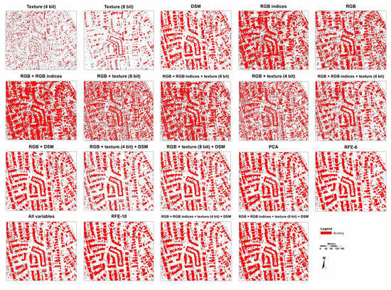
Classification performance using only one group of indices (i.e., RGB bands, texture, RGB indices or morphometric indices) varied in a wide range. Texture information was the weakest, worse when only RGB bands were used. Morphometric indices performed better on class level than on overall because DSM and its derivatives added valuable information especially in case of buildings. RGB indices had a relevant contribution in the improvement but on class level it was worse than the overall accuracy.

-

Combination of different group of indices ensured higher accuracy both on overall and class level. Best option is to use the morphometric indices with the RGB bands, it had >90% OA, PA, and UA.

-

Combining three types of indices provided the most efficient models, having >95% OA, PA, and UA. The RGB bands, RGB indices, morphometric indices and the 4 bit texture information had the largest (100% UA and 98% PA). In addition, 4 bit and 8 bit texture information had small differences in these combinations, and the most important to avoid their common application (both versions decrease the accuracy).

-

Model evaluation should contain the UA and PA values, and having several model solutions, visualization of these metrics helps to find the trade-offs between omission and commission errors. In addition, F1 an IoU can express it with a single value which helps to create ranks of accuracy.

-

RFE as variable selection method provided an importance rank, and both the six and ten variable sets were efficient, providing the same accuracy as including all variables (100% UA and 98% PA). We suggest using the fewest number of variables to avoid overfitting. However, our most important variables (nDSM, RGBVI, GLI, blue band from RGB, slope, VARI) can be different in other study areas, so the methodology and the careful and customized variable selection is more important.

-

Efficiency of this approach can be limited in areas where high buildings have large shadows and building roofs are flat. While shadows bias the spectral profiles, flat roofs will be identical with roads, pavements, and parking lots; thus, slope and aspect cannot discriminate buildings.

Results confirmed that archive images can provide appropriate data for urban sprawl monitoring focusing directly on the buildings.

References

1. Bramhe, V.S.; Ghosh, S.K.; Garg, P.K. Extraction of built-up area by combining textural features and spectral indices from landsat-8 multispectral image. ISPRS Int. Arch. Photogramm. Remote Sens. Spat. Inf. Sci. 2018, XLII–5, 727–733. [Google Scholar] [CrossRef] [Green Version]
2. Urban Development | Data. Available online: https://data.worldbank.org/topic/urban-development (accessed on 12 May 2020).
3. Urbanisation Worldwide | Knowledge for Policy. Available online: https://ec.europa.eu/knowledge4policy/foresight/topic/continuing-urbanisation/urbanisation-worldwide_en (accessed on 12 May 2020).
4. Orsini, H.F. Belgrade’s urban transformation during the 19th century: A space syntax approach. Geogr. Pannonica 2018, 22, 219–229. [Google Scholar] [CrossRef]
5. Maktav, D.; Erbek, F.S.; Jürgens, C. Remote sensing of urban areas. Int. J. Remote Sens. 2005, 26, 655–659. [Google Scholar] [CrossRef]
6. Müller, S.; Zaum, D.W. Robust building detection in aerial images. In Proceedings of the ISPRS Working Group III/4–5 and IV/3: “CMRT 2005”, Vienna, Austria, 29–30 August 2005; Volume XXXVI, pp. 143–148. [Google Scholar]
7. Lai, X.; Yang, J.; Li, Y.; Wang, M. A building extraction approach based on the fusion of LiDAR point cloud and elevation map texture features. Remote Sens. 2019, 11, 1636. [Google Scholar] [CrossRef] [Green Version]
8. Cilia, C.; Panigada, C.; Rossini, M.; Candiani, G.; Pepe, M.; Colombo, R. Mapping of asbestos cement roofs and their weathering status using hyperspectral aerial images. ISPRS Int. J. Geo Inf. 2015, 4, 928–941. [Google Scholar] [CrossRef] [Green Version]
9. Wilk, E.; Krówczyńska, M.; Pabjanek, P. Determinants influencing the amount of asbestos-cement roofing in Poland. Misc. Geogr. 2015, 19, 82–86. [Google Scholar] [CrossRef] [Green Version]
10. Szabó, S.; Burai, P.; Kovács, Z.; Szabó, G.; Kerényi, A.; Fazekas, I.; Paládi, M.; Buday, T.; Szabó, G. Testing algorithms for the identification of asbestos roofing based on hyperspectral data. Environ. Eng. Manag. J. 2014, 13, 2875–2880. [Google Scholar] [CrossRef]
11. Dian, C.; Pongrácz, R.; Incze, D.; Bartholy, J.; Talamon, A. Analysis of the urban heat island intensity based on air temperature measurements in a renovated part of Budapest (Hungary). Geogr. Pannonica 2019, 23, 277–288. [Google Scholar] [CrossRef] [Green Version]
12. Savic, S.; Unger, J.; Gál, T.; Milosevic, D.; Popov, Z. Urban heat island research of Novi Sad (Serbia): A review. Geogr. Pannonica 2013, 17, 32–36. [Google Scholar] [CrossRef] [Green Version]
13. Hayakawa, K.; Tang, N.; Nagato, E.; Toriba, A.; Lin, J.M.; Zhao, L.; Zhou, Z.; Qing, W.; Yang, X.; Mishukov, V.; et al. Long-term trends in urban atmospheric polycyclic aromatic hydrocarbons and nitropolycyclic aromatic hydrocarbons: China, Russia, and Korea from 1999 to 2014. Int. J. Environ. Res. Public Health 2020, 17, 431. [Google Scholar] [CrossRef] [Green Version]
14. Diao, B.; Ding, L.; Zhang, Q.; Na, J.; Cheng, J. Impact of urbanization on PM2.5-related health and economic loss in China 338 cities. Int. J. Environ. Res. Public Health 2020, 17, 990. [Google Scholar] [CrossRef] [PubMed] [Green Version]
15. Molnár, V.É.; Simon, E.; Tóthmérész, B.; Ninsawat, S.; Szabó, S. Air pollution induced vegetation stress—The air pollution tolerance index as a quick tool for city health evaluation. Ecol. Indic. 2020, 113, 106234. [Google Scholar] [CrossRef]
16. Xu, C.; Rahman, M.; Haase, D.; Wu, Y.; Su, M.; Pauleit, S. Surface runoff in urban areas: The role of residential cover and urban growth form. J. Clean. Prod. 2020, 262, 121421. [Google Scholar] [CrossRef]
17. Łopucki, R.; Klich, D.; Kitowski, I.; Kiersztyn, A. Urban size effect on biodiversity: The need for a conceptual framework for the implementation of urban policy for small cities. Cities 2020, 98. [Google Scholar] [CrossRef]
18. Chen, R.; Li, X.; Li, J. Object-based features for house detection from RGB high-resolution images. Remote Sens. 2018, 10, 451. [Google Scholar] [CrossRef] [Green Version]
19. Awrangjeb, M.; Ravanbakhsh, M.; Fraser, C.S. Automatic building detection using LIDAR data and multispectral imagery. In Proceedings of the International Conference on Digital Image Computing: Techniques and Applications (DICTA), Sydney, NSW, Australia, 1–3 December 2010; pp. 45–51. [Google Scholar] [CrossRef]
20. Vosselman, G. Fusion of laser scanning data, maps, and aerial photographs for building reconstruction. Int. Geosci. Remote Sens. Symp. 2002, 1, 85–88. [Google Scholar] [CrossRef]
21. Feng, Q.; Liu, J.; Gong, J. UAV Remote sensing for urban vegetation mapping using Random Forest and texture analysis. Remote Sens. 2015, 7, 1074–1094. [Google Scholar] [CrossRef] [Green Version]
22. Gavankar, N.L.; Ghosh, S.K. Automatic building footprint extraction from high-resolution satellite image using mathematical morphology. Eur. J. Remote Sens. 2018, 51, 182–193. [Google Scholar] [CrossRef] [Green Version]
23. San, D.K.; Turker, M. Building extraction from high resolution satellite images using Hough transform. ISPRS Int. Arch. Photogramm. Remote Sens. Spat. Inf. Sci. 2010, XXXVIII, 1063–1068. [Google Scholar]
24. Sohn, G.; Dowman, I. Data fusion of high-resolution satellite imagery and LiDAR data for automatic building extraction. ISPRS J. Photogramm. Remote Sens. 2007, 62, 43–63. [Google Scholar] [CrossRef]
25. Zhang, K.; Yan, J.; Chen, S.C. Automatic construction of building footprints from airborne LIDAR data. IEEE Trans. Geosci. Remote Sens. 2006, 44, 2523–2533. [Google Scholar] [CrossRef] [Green Version]
26. Quang, N.T.; Sang, D.V.; Thuy, N.T.; Binh, H.T.T. An efficient framework for pixel-wise building segmentation from aerial images. In Proceedings of the 6th International Symposium on Information and Communication Technology ACM, Hue City, Vietnam, 3–4 December 2015; pp. 282–287. [Google Scholar] [CrossRef]
27. Jaynes, C.; Riseman, E.; Hanson, A. Recognition and reconstruction of buildings from multiple aerial images. Comput. Vis. Image Underst. 2003, 90, 68–98. [Google Scholar] [CrossRef]
28. Fischer, A.; Kolbe, T.H.; Lang, F.; Cremers, A.B.; Förstner, W.; Plümer, L.; Steinhage, V. Extracting buildings from aerial images using hierarchical aggregation in 2D and 3D. Comput. Vis. Image Underst. 1998, 72, 185–203. [Google Scholar] [CrossRef] [Green Version]
29. Sirmaçek, B.; Ünsalan, C. Building detection from aerial images using invariant color features and shadow information. In Proceedings of the 23rd International Symposium on Computer and Information Sciences, ISCIS 2008, Istanbul, Turkey, 27–29 October 2008; pp. 105–110. [Google Scholar] [CrossRef]
30. Vogtle, T.; Steinle, E. 3D modelling of buildings using laser scanning and spectral information. Int. Arch. Photogramm. Remote Sens. 2000, 33, 927–934. [Google Scholar]
31. Li, Y.; Wu, H. Adaptive building edge detection by combining LiDAR data and aerial images. Int. Arch. Photogramm. Remote Sens. Spat. Inf. Sci. 2008, 37, 197–202. [Google Scholar]
32. Li, E.; Femiani, J.; Xu, S.; Zhang, X.; Wonka, P. Band images using higher order CRF. Iee Trans. Geosci. Remote Sens. 2015, 53, 4483–4495. [Google Scholar] [CrossRef]
33. Szabó, Z.; Tóth, C.A.; Holb, I.; Szabó, S. Aerial laser scanning data as a source of terrain modeling in a fluvial environment: Biasing factors of terrain height accuracy. Sensors 2020, 20, 63. [Google Scholar] [CrossRef] [Green Version]
34. Rottensteiner, F.; Trinder, J.; Clode, S.; Kubik, K. Building detection by fusion of airborne laser scanner data and multi-spectral images: Performance evaluation and sensitivity analysis. ISPRS J. Photogramm. Remote Sens. 2007, 62, 135–149. [Google Scholar] [CrossRef]
35. Tomljenovic, I.; Tiede, D.; Blaschke, T. A building extraction approach for airborne laser scanner data utilizing the object based image analysis paradigm. Int. J. Appl. Earth Obs. Geoinf. 2016, 52, 137–148. [Google Scholar] [CrossRef] [Green Version]
36. Burai, P.; Bekő, L.; Lénárt, C.; Tomor, T.; Kovács, Z. Individual tree species classification using airborne hyperspectral imagery and lidar data. In Proceedings of the 2019 10th Workshop on Hyperspectral Imaging and Signal Processing: Evolution in Remote Sensing (WHISPERS), Amsterdam, The Netherlands, 24–26 September 2019; pp. 1–4. [Google Scholar] [CrossRef]
37. Ambrus, A.; Burai, P.; Bekő, L.; Jolánkai, M. Precíziós növénytermesztési technológiák és nagy felbontású légi távérzékelt adatok alkalmazhatósága az őszi búza termesztésében. Acta Agron. Óváriensis 2017, 58, 85–104. [Google Scholar]
38. Moussa, A.; El-Sheimy, N. A new object based method for automated extraction of urban objects from airborne sensors data. ISPRS Int. Arch. Photogramm. Remote Sens. Spat. Inf. Sci. 2012, XXXIX-B3, 309–314. [Google Scholar] [CrossRef] [Green Version]
39. Szabó, S.; Enyedi, P.; Horváth, M.; Kovács, Z.; Burai, P.; Csoknyai, T.; Szabó, G. Automated registration of potential locations for solar energy production with Light Detection and Ranging (LiDAR) and small format photogrammetry. J. Clean. Prod. 2016, 112, 3820–3829. [Google Scholar] [CrossRef]
40. Abe, J.; Marzolff, I.; Ries, J. Small-Format Aerial Photography; Elsevier Inc.: Amsterdam, The Netherlands, 2010; ISBN 9780444532602. [Google Scholar]
41. Szabó, G.; Bertalan, L.; Barkóczi, N.; Kovács, Z.; Burai, P.; Lénárt, C. Zooming on Aerial Survey. In Small Flying Drones: Applications for Geographic Observation; Casagrande, G., Sik, A., Szabó, G., Eds.; Springer International Publishing: Cham, Switzerland, 2018; pp. 91–126. ISBN 978-3-319-66577-1. [Google Scholar]
42. Shen, X.; Cao, L.; Yang, B.; Xu, Z.; Wang, G. Estimation of forest structural attributes using spectral indices and point clouds from UAS-based multispectral and RGB imageries. Remote Sens. 2019, 11, 800. [Google Scholar] [CrossRef] [Green Version]
43. Luo, N.; Wan, T.; Hao, H.; Lu, Q. Fusing high-spatial-resolution remotely sensed imagery and OpenStreetMap data for land cover classification over urban areas. Remote Sens. 2019, 11, 88. [Google Scholar] [CrossRef] [Green Version]
44. Pessoa, G.G.; Amorim, A.; Galo, M.; Galo, M.d.L.B.T. Photogrammetric point cloud classification based on geometric and radiometric data integration. Bol. Cienc. Geod. 2019, 25, 1–17. [Google Scholar] [CrossRef] [Green Version]
45. Schwind, M.; Starek, M. Structure-from-motion photogrammetry. Gim Int. 2017, 31, 36–39. [Google Scholar]
46. Jiang, S.; Jiang, W. Efficient SfM for oblique UAV images: From match pair selection to geometrical verification. Remote Sens. 2018, 10, 1246. [Google Scholar] [CrossRef] [Green Version]
47. Grigillo, D.; Kanjir, U. Urban object extraction from digital surface model and digital aerial images. ISPRS Ann. Photogramm. Remote Sens. Spat. Inf. Sci. 2012, 1, 215–220. [Google Scholar] [CrossRef] [Green Version]
48. Rau, J.Y.; Jhan, J.P.; Hsu, Y.C. Analysis of oblique aerial images for land cover and point cloud classification in an Urban environment. IEEE Trans. Geosci. Remote Sens. 2015, 53, 1304–1319. [Google Scholar] [CrossRef]
49. Haala, N.; Brenner, C. Extraction of buildings and trees in urban environments. ISPRS J. Photogramm. Remote Sens. 1999, 54, 130–137. [Google Scholar] [CrossRef]
50. Yan, G.; Mas, J.F.; Maathuis, B.H.P.; Xiangmin, Z.; van Dijk, P.M. Comparison of pixel-based and object-oriented image classification approaches—A case study in a coal fire area, Wuda, Inner Mongolia, China. Int. J. Remote Sens. 2006, 27, 4039–4055. [Google Scholar] [CrossRef]
51. Liu, D.; Xia, F. Assessing object-based classification: Advantages and limitations. Remote Sens. Lett. 2010, 1, 187–194. [Google Scholar] [CrossRef]
52. Möller, M.; Lymburner, L.; Volk, M. The comparison index: A tool for assessing the accuracy of image segmentation. Int. J. Appl. Earth Obs. Geoinf. 2007, 9, 311–321. [Google Scholar] [CrossRef]
53. Blaschke, T.; Lang, S.; Lorup, E.; Strobl, J.; Zeil, P. Object-oriented image processing in an integrated GIS/remote sensing environment and perspectives for environmental applications. Environmental information for planning, politics and the public. Environ. Inf. Plan. Polit. Public 2000, 2, 555–570. [Google Scholar]
54. Adams, R.; Bischof, L. Seeded region growing. IEEE Trans. Pattern Anal. Mach. Intell. 1994, 16, 641–647. [Google Scholar] [CrossRef] [Green Version]
55. Hossain, M.D.; Chen, D. Segmentation for Object-Based Image Analysis (OBIA): A review of algorithms and challenges from remote sensing perspective. ISPRS J. Photogramm. Remote Sens. 2019, 150, 115–134. [Google Scholar] [CrossRef]
56. Tarsha-Kurdi, F.; Landes, T.; Grussenmeyer, P. Joint combination of point cloud and DSM for 3D building reconstruction using airborne laser scanner data. In Proceedings of the 2007 Urban Remote Sensing Joint Event (URBAN/URS), Paris, France, 11–13 April 2007; pp. 3–10. [Google Scholar] [CrossRef] [Green Version]
57. Awrangjeb, M.; Zhang, C.; Fraser, C.S. Automatic extraction of building roofs using LIDAR data and multispectral imagery. ISPRS J. Photogramm. Remote Sens. 2013, 83, 1–18. [Google Scholar] [CrossRef] [Green Version]
58. Maltezos, E.; Ioannidis, C. Automatic detection of building points from LiDAR and dense image matching point clouds. ISPRS Ann. Photogramm. Remote Sens. Spat. Inf. Sci. 2015, 2, 33–40. [Google Scholar] [CrossRef] [Green Version]
59. Mahphood, A.; Arefi, H. Virtual first and last pulse method for building detection from dense LiDAR point clouds. Int. J. Remote Sens. 2020, 41, 1067–1092. [Google Scholar] [CrossRef]
60. Shorter, N.; Kasparis, T. Automatic vegetation identification and building detection from a single nadir aerial image. Remote Sens. 2009, 1, 731–757. [Google Scholar] [CrossRef] [Green Version]
61. Shi, F.; Xi, Y.; Li, X.; Duan, Y. An automation system of rooftop detection and 3D building modeling from aerial images. J. Intell. Robot. Syst. Theory Appl. 2011, 62, 383–396. [Google Scholar] [CrossRef]
62. Agisoft LLC. Agisoft Metashape User Manual: Professional Edition, Version 1.5. 2019. Available online: https://www.agisoft.com/pdf/metashape-pro_1_5_en.pdf (accessed on 27 May 2020).
63. Liu, H.; Wu, C. Developing a scene-based triangulated irregular network (TIN) technique for individual tree crown reconstruction with LiDAR data. Forests 2020, 11, 28. [Google Scholar] [CrossRef] [Green Version]
64. Park, S.W.; Linsen, L.; Kreylos, O.; Owens, J.D.; Hamann, B. Discrete sibson interpolation. IEEE Trans. Vis. Comput. Graph. 2006, 12, 243–252. [Google Scholar] [CrossRef] [PubMed]
65. Zhang, W.; Qi, J.; Wan, P.; Wang, H.; Xie, D.; Wang, X.; Yan, G. An easy-to-use airborne LiDAR data filtering method based on cloth simulation. Remote Sens. 2016, 8, 501. [Google Scholar] [CrossRef]
66. Yan, L.; Li, Z.; Xie, H. Segmentation of unorganized point cloud from terrestrial laser scanner in urban region. In Proceedings of the 18th International Conference on Geoinformatics, Beijing, China, 18–20 June 2010; pp. 1–5. [Google Scholar] [CrossRef]
67. Jochem, A.; Höfle, B.; Rutzinger, M.; Pfeifer, N. Automatic roof plane detection and analysis in airborne LiDAR point clouds for solar potential assessment. Sensors 2009, 9, 5241–5262. [Google Scholar] [CrossRef]
68. Hunt, E.R.; Dean Hively, W.; Fujikawa, S.J.; Linden, D.S.; Daughtry, C.S.T.; McCarty, G.W. Acquisition of NIR-green-blue digital photographs from unmanned aircraft for crop monitoring. Remote Sens. 2010, 2, 290–305. [Google Scholar] [CrossRef] [Green Version]
69. Zhang, X.; Zhang, F.; Qi, Y.; Deng, L.; Wang, X.; Yang, S. New research methods for vegetation information extraction based on visible light remote sensing images from an unmanned aerial vehicle (UAV). Int. J. Appl. Earth Obs. Geoinf. 2019, 78, 215–226. [Google Scholar] [CrossRef]
70. Yuan, H.; Liu, Z.; Cai, Y.; Zhao, B. Research on vegetation information extraction from visible UAV remote sensing images. In Proceedings of the 5th International Workshop on Earth Observation and Remote Sensing Applications (EORSA), Xi’an, China, 18–20 June 2018; pp. 1–5. [Google Scholar] [CrossRef]
71. Zhu, Y.; Yang, K.; Pan, E.; Yin, X.; Zhao, J. Extraction and analysis of urban vegetation information based on remote sensing image. In Proceedings of the 26th International Conference on Geoinformatics, Kunming, China, 28–30 June 2018; pp. 1–10. [Google Scholar] [CrossRef]
72. Motohka, T.; Nasahara, K.N.; Oguma, H.; Tsuchida, S. Applicability of green-red vegetation index for remote sensing of vegetation phenology. Remote Sens. 2010, 2, 2369–2387. [Google Scholar] [CrossRef] [Green Version]
73. Louhaichi, M.; Borman, M.M.; Johnson, D.E. Spatially located platform and aerial photography for documentation of grazing impacts on wheat. Geocarto Int. 2001, 16, 65–70. [Google Scholar] [CrossRef]
74. Gitelson, A.A.; Kaufman, Y.J.; Stark, R.; Rundquist, D. Novel algorithms for remote estimation of vegetation fraction. Remote Sens. Environ. 2002, 80, 76–87. [Google Scholar] [CrossRef] [Green Version]
75. Lussem, U.; Bolten, A.; Gnyp, M.L.; Jasper, J.; Bareth, G. Evaluation of RGB-based vegetation indices from UAV imagery to estimate forage yield in Grassland. ISPRS Int. Arch. Photogramm. Remote Sens. Spat. Inf. Sci. 2018, 42, 1215–1219. [Google Scholar] [CrossRef] [Green Version]
76. Hunt, E.R.; Cavigelli, M.; Daughtry, C.S.T.; McMurtrey, J.E.; Walthall, C.L. Evaluation of digital photography from model aircraft for remote sensing of crop biomass and nitrogen status. Precis. Agric. 2005, 6, 359–378. [Google Scholar] [CrossRef]
77. Tucker, C.J. Red and photographic infrared linear combinations for monitoring vegetation. Remote Sens. Environ. 1979, 8, 127–150. [Google Scholar] [CrossRef] [Green Version]
78. Bendig, J.; Yu, K.; Aasen, H.; Bolten, A.; Bennertz, S.; Broscheit, J.; Gnyp, M.L.; Bareth, G. Combining UAV-based plant height from crop surface models, visible, and near infrared vegetation indices for biomass monitoring in barley. Int. J. Appl. Earth Obs. Geoinf. 2015, 39, 79–87. [Google Scholar] [CrossRef]
79. Bareth, G.; Bolten, A.; Gnyp, M.L.; Reusch, S.; Jasper, J. Comparison of uncalibrated RGBVI with spectrometer-based NDVI derived from UAV sensing systems on field scale. ISPRS Int. Arch. Photogramm. Remote Sens. Spat. Inf. Sci. 2016, 41, 837–843. [Google Scholar] [CrossRef]
80. Kupidura, P. The comparison of different methods of texture analysis for their efficacy for land use classification in satellite imagery. Remote Sens. 2019, 11, 1233. [Google Scholar] [CrossRef] [Green Version]
81. Chaurasia, K.; Garg, P.K. The role of texture information and data fusion in topographic objects extraction from satellite data. Geod. Cartogr. 2014, 40, 116–121. [Google Scholar] [CrossRef] [Green Version]
82. Zhang, X.; Cui, J.; Wang, W.; Lin, C. A study for texture feature extraction of high-resolution satellite images based on a direction measure and gray level co-occurrence matrix fusion algorithm. Sensors 2017, 17, 1474. [Google Scholar] [CrossRef] [Green Version]
83. Weszka, J.S.; Dyer, C.R.; Rosenfeld, A. A comparative study of texture measures for terrain classification. IEEE Trans. Syst. Man Cybern. 1976, SMC-6, 269–285. [Google Scholar] [CrossRef]
84. Zhang, Y. Optimisation of building detection in satellite images by combining multispectral classification and texture filtering. ISPRS J. Photogramm. Remote Sens. 1999, 54, 50–60. [Google Scholar] [CrossRef]
85. Clausi, D.A.; Zhao, Y. Rapid extraction of image texture by co-occurrence using a hybrid data structure. Comput. Geosci. 2002, 28, 763–774. [Google Scholar] [CrossRef]
86. Haralick, R.; Shanmugam, K.; Dinstein, I. Textural features for image classification. IEEE Trans. Syst. Man Cybern. 1973, SMC-3, 610–621. [Google Scholar] [CrossRef] [Green Version]
87. Kabir, S.; He, D.C.; Sanusi, M.A.; Wan Hussina, W.M.A. Texture analysis of IKONOS satellite imagery for urban land use and land cover classification. Imaging Sci. J. 2010, 58, 163–170. [Google Scholar] [CrossRef]
88. Tang, X. Texture information in run-length matrices. IEEE Trans. Image Process. 1998, 7, 1602–1609. [Google Scholar] [CrossRef] [PubMed] [Green Version]
89. Galloway, M.M. Texture analysis using gray level run lengths. Comput. Graph. Image Process. 1975, 4, 172–179. [Google Scholar] [CrossRef]
90. Bechtel, B.; Ringeler, A.; Böhner, J. Segmentation for object extraction of treed using MATLAB and SAGA. Hamburg. Beiträge Zur Phys. Geogr. Und Landsch. 2008, 19, 1–12. [Google Scholar]
91. R: The R Project for Statistical Computing. Available online: https://www.r-project.org/ (accessed on 13 May 2020).
92. Revelle, W. Psych: Procedures for Personality and Psychological Research, Northwerstern University, Evanston, Illinois, USA, R Package Version 1.9.12. Available online: https://cran.r-project.org/web/packages/psych/psych.pdf (accessed on 13 May 2020).
93. Bernaards, C.A.; Jennrich, R.I. Gradient projection algorithms and software for arbitrary rotation criteria in factor analysis. Educ. Psychol. Meas. 2005, 65, 770–790. [Google Scholar] [CrossRef]
94. Chen, Q.; Meng, Z.; Liu, X.; Jin, Q.; Su, R. Decision variants for the automatic determination of optimal feature subset in RF-RFE. Genes 2018, 9, 301. [Google Scholar] [CrossRef] [Green Version]
95. Kuhn, M.; Wing, J.; Weston, S.; Williams, A.; Keefer, C.; Engelhardt, A.; Cooper, T.; Mayer, Z.; Kenkel, B.; R Core Team; et al. Package ‘Caret’: Classification and Regression Training. R Package Version 6.0–86. 2020. Available online: https://cran.r-project.org/web/packages/caret/caret.pdf (accessed on 13 May 2020).
96. Breiman, L. Random Forests. Mach. Learn. 2001, 45, 5–32. [Google Scholar] [CrossRef] [Green Version]
97. Cortes, C.; Vapnik, V. Support-vector networks. Mach. Learn. 1995, 20, 273–297. [Google Scholar] [CrossRef]
98. Crammer, K. On the algorithmic implementation of multiclass kernel-based vector machines. J. Mach. Learn. Res. JMLR 2002, 2, 265–292. [Google Scholar]
99. Lee, Y.; Lin, Y.; Wahba, G. Multicategory support vector machines: Theory and application to the classification of microarray data and satellite radiance data. J. Am. Stat. Assoc. 2004, 99, 67–81. [Google Scholar] [CrossRef] [Green Version]
100. Tong, J.C. Cross-Validation. Encycl. Syst. Biol. 2013, 508. [Google Scholar] [CrossRef]
101. Friedman, J.H. Multivariate Adaptive Regression Splines. Ann. Stat. 1991, 19, 1–67. [Google Scholar] [CrossRef]
102. Rotigliano, E.; Martinello, C.; Agnesi, V.; Conoscenti, C. Evaluation of debris flow susceptibility in El Salvador (CA): A comparisobetween multivariate adaptive regression splines (MARS) and binary logistic regression (BLR). Hung. Geogr. Bull. 2018, 67, 361–373. [Google Scholar] [CrossRef] [Green Version]
103. Golub, G.H.; Heath, M.; Wahba, G. Generalized cross-validation as a method for choosing a good ridge parameter. Technometrics 1979, 21, 215–223. [Google Scholar] [CrossRef]
104. Barker, M.; Rayens, W. Partial least squares for discrimination. J. Chemom. 2003, 17, 166–173. [Google Scholar] [CrossRef]
105. Yeh, C.H.; Spiegelman, C.H. Partial least squares and classification and regression trees. Chemom. Intell. Lab. Syst. 1994, 22, 17–23. [Google Scholar] [CrossRef]
106. Liaw, A.; Wiener, M. Classification and Regression by randomForest. R News 2002, 2, 18–22. [Google Scholar]
107. Therneau, T.; Atkinson, B.; Ripley, B. rpart: Recursive Partitioning for Classification, Regression and Survival Trees. R Package Version 4.1-15. 2019. Available online: https://cran.r-project.org/web/packages/rpart/rpart.pdf (accessed on 22 May 2020).
108. Mevik, B.-H.; Wehrens, R.; Liland, H. pls: Partial Least Squares and Principal Component Regression, R Package Version 2.7–2. 2019. Available online: https://cran.r-project.org/web/packages/pls/pls.pdf (accessed on 22 May 2020).
109. Meyer, D.; Dimitriadou, E.; Hornik, K.; Weingessel, A.; Leisch, F. e1071: Misc Functions of the Department of Statistics, Probability Theory Group (Formerly: E1071), TU Wien, R Package Version 1.7–3. 2019. Available online: https://cran.r-project.org/web/packages/e1071/e1071.pdf (accessed on 22 May 2020).
110. Kim, J.H. Estimating classification error rate: Repeated cross-validation, repeated hold-out and bootstrap. Comput. Stat. Data Anal. 2009, 53, 3735–3745. [Google Scholar] [CrossRef]
111. Molinaro, A.M.; Simon, R.; Pfeiffer, R.M. Prediction error estimation: A comparison of resampling methods. Bioinformatics 2005, 21, 3301–3307. [Google Scholar] [CrossRef] [PubMed] [Green Version]
112. Pontius, R.G.; Millones, M. Death to Kappa: Birth of quantity disagreement and allocation disagreement for accuracy assessment. Int. J. Remote Sens. 2011, 32, 4407–4429. [Google Scholar] [CrossRef]
113. Powers, D.M.W. Evaluation: From precision, recall and F-Factor to ROC, informedness, markedness & correlation. J. Mach. Learn. Technol. 2007, 2, 37–63. [Google Scholar]
114. Tan, P.-N.; Steinbach, M.; Karpatne, A.; Kumar, V. Introduction to Data Mining; Pearson Publisher, 2005; 792p, Available online: https://www-users.cs.umn.edu/~kumar001/dmbook/index.php (accessed on 8 July 2020).
115. Congalton, R.G. A review of assessing the accuracy of classifications of remotely sensed data. Remote Sens. Environ. 1991, 37, 35–46. [Google Scholar] [CrossRef]
116. ISPRS Test Project on Urban Classification and 3D Building Reconstruction. Available online: http://www2.isprs.org/commissions/comm3/wg4/detection-and-reconstruction.html (accessed on 8 July 2020).
117. Varga, K.; Szabó, S.; Szabó, G.; Dévai, G.; Tóthmérész, B. Improved land cover mapping using aerial photographs and satellite images. Open Geosci. 2015, 7, 15–26. [Google Scholar] [CrossRef] [Green Version]
118. Cots-Folch, R.; Aitkenhead, M.J.; Martínez-Casasnovas, J.A. Mapping land cover from detailed aerial photography data using textural and neural network analysis. Int. J. Remote Sens. 2007, 28, 1625–1642. [Google Scholar] [CrossRef]
119. Al-Kofahi, S.; Steele, C.; VanLeeuwen, D.; Hilaire, R.S. Mapping land cover in urban residential landscapes using very high spatial resolution aerial photographs. Urban For. Urban Green. 2012, 11, 291–301. [Google Scholar] [CrossRef]
120. Li, X.; Myint, S.W.; Zhang, Y.; Galletti, C.; Zhang, X.; Turner, B.L. Object-based land-cover classification for metropolitan Phoenix, Arizona, using aerial photography. Int. J. Appl. Earth Obs. Geoinf. 2014, 33, 321–330. [Google Scholar] [CrossRef]
121. Deng, J.S.; Wang, K.; Li, J.; Deng, Y.H. Urban land use change detection using multisensor satellite images project supported by the national Natural Science Foundation of China (NSFC) (No. 30571112). Pedosphere 2009, 19, 96–103. [Google Scholar] [CrossRef]
122. Szabó, L.; Burai, P.; Deák, B.; Dyke, G.J.; Szabó, S. Assessing the efficiency of multispectral satellite and airborne hyperspectral images for land cover mapping in an aquatic environment with emphasis on the water caltrop (Trapa natans). Int. J. Remote Sens. 2019, 40, 5192–5215. [Google Scholar] [CrossRef]
123. Bakuła, K.; Kupidura, P.; Jełowicki, Ł. Testing of land cover classification from multispectral airborne laser scanning data. ISPRS Int. Arch. Photogramm. Remote Sens. Spat. Inf. Sci. 2016, 41, 161–169. [Google Scholar] [CrossRef]
124. Albregtsen, F. Statistical texture measures computed from GLCM–Matrices. Image Processing Lab. Dep. Inform. Oslo Univ. Oslo 2008, 5, 1–14. [Google Scholar]
125. Pawade, P.W. Texture image classification using Support Vector Machine. Int. J. Comput. Technol. Appl. 2012, 03, 71–75. [Google Scholar]
126. Bofana, J.; Zhang, M.; Nabil, M.; Wu, B.; Tian, F.; Liu, W.; Zeng, H.; Zhang, N.; Nangombe, S.S.; Cipriano, S.A.; et al. Comparison of different cropland classification methods under diversified agroecological conditions in the zambezi river basin. Remote Sens. 2020, 12, 2096. [Google Scholar] [CrossRef]
127. Xu, F.; Li, Z.; Zhang, S.; Huang, N.; Quan, Z.; Zhang, W.; Liu, X.; Jiang, X.; Pan, J.; Prishchepov, A.V. Mapping winter wheat with combinations of temporally aggregated Sentinel-2 and Landsat-8 data in Shandong Province, China. Remote Sens. 2020, 12, 2065. [Google Scholar] [CrossRef]
128. Van Leeuwen, B.; Mezosi, G.; Tobak, Z.; Szatmári, J.; Barta, K. Identification of inland excess water floodings using an artificial neural network. Carpathian J. Earth Environ. Sci. 2012, 7, 173–180. [Google Scholar]
129. Hang, R.; Li, Z.; Ghamisi, P.; Hong, D.; Xia, G.; Liu, Q. Classification of hyperspectral and LiDAR data using coupled CNNs. IEEE Trans. Geosci. Remote Sens. 2020, 58, 4939–4950. [Google Scholar] [CrossRef] [Green Version]
130. Hang, R.; Liu, Q.; Hong, D.; Ghamisi, P. Cascaded recurrent neural networks for hyperspectral image classification. IEEE Trans. Geosci. Remote Sens. 2019, 57, 5384–5394. [Google Scholar] [CrossRef] [Green Version]
131. Hasan, H.; Shafri, H.Z.M.; Habshi, M. A Comparison between Support Vector Machine (SVM) and Convolutional Neural Network (CNN) models for hyperspectral image classification. IOP Conf. Ser. Earth Environ. Sci. 2019, 357. [Google Scholar] [CrossRef] [Green Version]
132. Huang, L.; An, R.; Zhao, S.; Jiang, T.; Hu, H. A deep learning-based robust change detection approach for very high resolution remotely sensed images with multiple features. Remote Sens. 2020, 12, 1441. [Google Scholar] [CrossRef]
133. Zhang, P.; Ke, Y.; Zhang, Z.; Wang, M.; Li, P.; Zhang, S. Urban land use and land cover classification using novel deep learning models based on high spatial resolution satellite imagery. Sensors 2018, 18, 3717. [Google Scholar] [CrossRef] [PubMed] [Green Version]
134. Zhang, L.; Xia, G.S.; Wu, T.; Lin, L.; Tai, X.C. Deep Learning for remote sensing image understanding. J. Sens. 2016, 2016. [Google Scholar] [CrossRef]
135. Chen, G.; Zhang, X.; Wang, Q.; Dai, F.; Gong, Y.; Zhu, K. Symmetrical dense-shortcut deep fully convolutional networks for semantic segmentation of very-high-resolution remote sensing images. IEEE J. Sel. Top. Appl. Earth Obs. Remote Sens. 2018, 11, 1633–1644. [Google Scholar] [CrossRef]
136. Ma, L.; Liu, Y.; Zhang, X.; Ye, Y.; Yin, G.; Johnson, B.A. Deep learning in remote sensing applications: A meta-analysis and review. ISPRS J. Photogramm. Remote Sens. 2019, 152, 166–177. [Google Scholar] [CrossRef]
137. Kuhn, M.; Johnson, K. Over-fitting and model tuning. In Applied Predictive Modeling; Springer: New York, NY, USA, 2013; pp. 61–92. [Google Scholar]
138. Hawkins, D.M. The Problem of Overfitting. J. Chem. Inf. Comput. Sci. 2004, 44, 1–12. [Google Scholar] [CrossRef] [PubMed]
139. Deng, B.C.; Yun, Y.H.; Liang, Y.Z.; Cao, D.S.; Xu, Q.S.; Yi, L.Z.; Huang, X. A new strategy to prevent over-fitting in partial least squares models based on model population analysis. Anal. Chim. Acta 2015, 880, 32–41. [Google Scholar] [CrossRef] [PubMed]
140. Reunanen, J. Overfitting in making comparisons between variable selection methods. J. Mach. Learn. Res. 2003, 3, 1371–1382. [Google Scholar]
141. Viswanathan, V.; Viswanathan, S. R Data Analysis Cookbook; Packt Publishing: Birmingham, UK, 2015. [Google Scholar]
142. Han, H.; Jiang, X. Overcome support vector machine diagnosis overfitting. Cancer Inform. 2014, 13s1, CIN.S13875. [Google Scholar] [CrossRef] [Green Version]
143. Khuntia, S.; Mujtaba, H.; Patra, C.; Farooq, K.; Sivakugan, N.; Das, B.M. Prediction of compaction parameters of coarse grained soil using multivariate adaptive regression splines (MARS). Int. J. Geotech. Eng. 2015, 9, 79–88. [Google Scholar] [CrossRef]
144. Tharwat, A. Classification assessment methods. Appl. Comput. Inform. 2018. [Google Scholar] [CrossRef]
145. Dong, Y.; Zhang, L.; Cui, X.; Ai, H.; Xu, B. Extraction of buildings from multiple-view aerial images using a feature-level-fusion strategy. Remote Sens. 2018, 10, 1947. [Google Scholar] [CrossRef] [Green Version]
Figure 1. Location of study area.
Remotesensing 12 02397 g001
Figure 2. Example of segments on different land cover classes.
Remotesensing 12 02397 g002
Figure 3. Variables and workflow.
Remotesensing 12 02397 g003
Figure 4. Improvement of overall classification accuracy (OA) by the number of variables. Variables are ranked based on recursive feature elimination determined by 10-fold repeated cross-validation in 3 repetitions (o: selected variable sets; : best OA with 30 variables).
Remotesensing 12 02397 g004
Figure 5. Classification accuracies using different variable sets and classifiers. Boxplots represent the medians (•), interquartile ranges, minimums, maximums (whiskers), and outliers (o) based on 30 models of repeated k-fold cross-validation (RKCV).
Remotesensing 12 02397 g005
Figure 6. Classification accuracies using different variable sets and classifiers ordered by decreasing OA medians: (a) ranking by random forest (RF) models; (b) ranking by the best performing models). Boxplots represent the medians (), interquartile ranges, minimums, maximums (whiskers), and outliers (o) based on 30 models of RKCV.
Remotesensing 12 02397 g006
Figure 7. Classification accuracies on category level based on the maps generated by RF models and independent testing dataset (input variables: rgb: visible bands; i: RGB indices, t: texture information, pca: principal components, d: morphometric indices, rfe: selected variables with recursive feature elimination; dashed red line: accuracies >95%).
Remotesensing 12 02397 g007
Figure 8. F1-values based on the maps generated by RF models and the independent test dataset (input variables: rgb: visible bands; i: RGB indices, t: texture information, pca: principal components, d: morphometric indices, rfe: selected variables with recursive feature elimination; dashed red line: accuracies >95%).
Remotesensing 12 02397 g008
Figure 9. Building representations in the study area using different variable sets and random forest classifier (input variables: RGB: visible bands; RGB indices, texture: texture information, PCA: principal component analysis, DSM: DSM derivatives as morphometric indices, RFE: selected variables with recursive feature elimination).
Remotesensing 12 02397 g009
Figure 10. The orthophoto of the study area in Toronto (a) and the result of building extraction (b) of the ISPRS Benchmark Dataset (TP: true positive; FN: false negative; FP: false positive).
Remotesensing 12 02397 g010