Ionospheric S4 Scintillations from GNSS Radio Occultation (RO) at Slant Path

Abstract

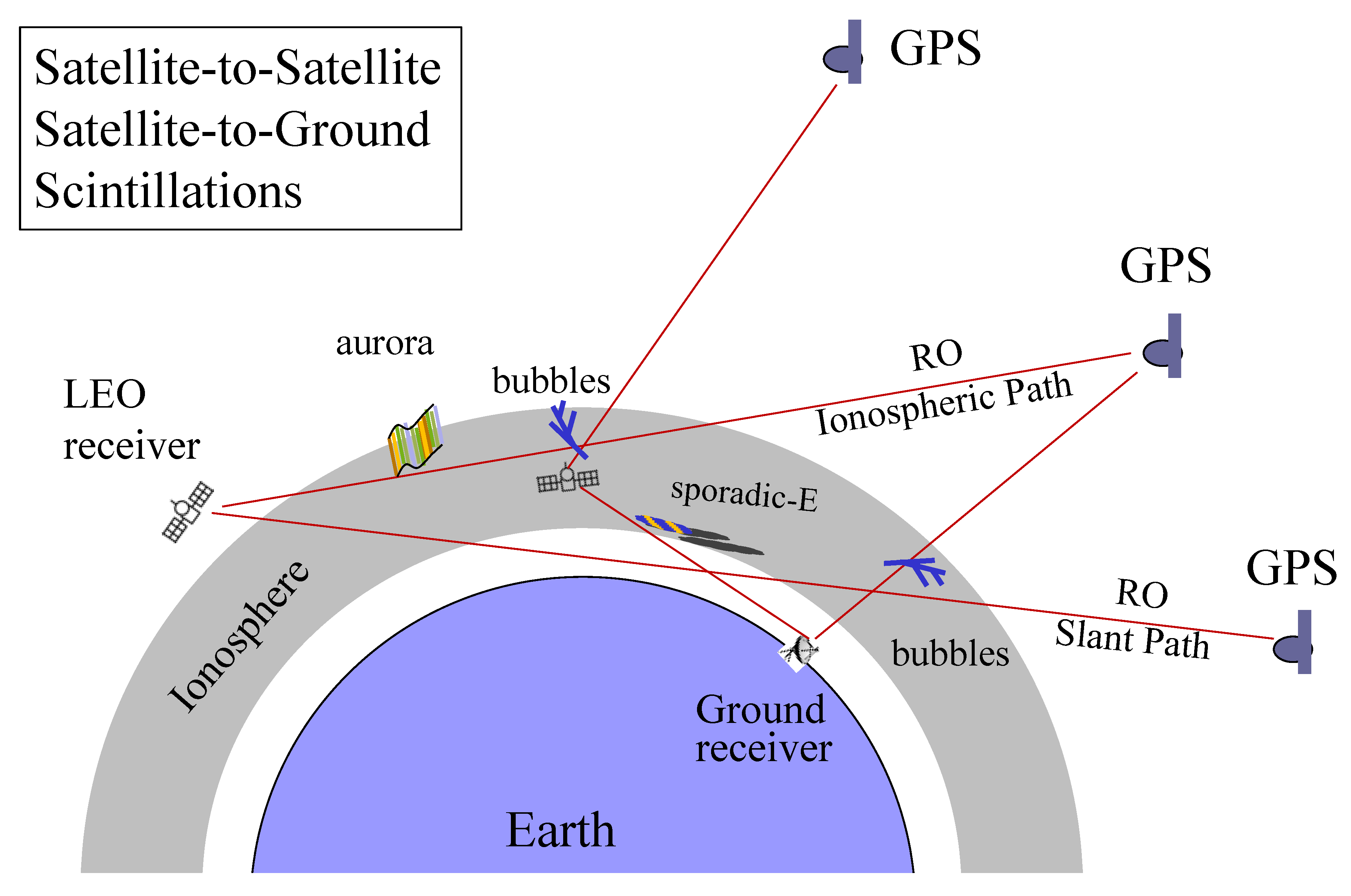
1. Introduction
2. Data and Method
2.1. 50–Hz RO Data
2.2. S4 Calculation and Aggregation
2.3. RO Slant Views and Smearing Effects on Scintillations
3. Results
3.1. Sporadic–E (Es)
3.2. Equatorial Plasma Bubbles (EPBs) and Equatorial Spread–F (ESF)
3.3. Polar Scintillations
3.4. Solar–Cycle Variations
4. Discussions
4.1. Effects of Geo–Registration and Structured Disturbances
4.2. GNSS–RO S4 and Phase () Scintillations
4.3. Implication for Scintillation Nowcast
5. Conclusions and Future Work
- (1)
- Es–induced S4 scintillations and their impacts on the ground–based receivers are stronger in the summer hemisphere with a significant diurnal variation;
- (2)
- GNSS–RO S4 scintillations from the slant path at ht = 30 km show the geographical and seasonal variations similar to the observed climatology of ESF/EPBs, which are consistent with the scintillations found by ground–based receivers. The enhanced S4 varies significantly with local time and magnetic dip angle;
- (3)
- the polar S4 scintillations are weak in all seasons, as inferred from GNSS–RO S4 at ht = 30 km;
- (4)
- a significant solar–cycle variation is found in the Es–induced daytime scintillations with a lower S4 value during the solar maximum. However, at high latitudes, the S4 variation is positively correlated with the solar cycle. The nighttime S4 exhibits a strong semiannual variation at low latitudes with a positive correlation with the solar cycle.
Supplementary Materials
Funding
Acknowledgments
Conflicts of Interest
References
- Kintner, M.P.; Ledvina, B.M.; de Paula, E.R. GPS and ionospheric scintillations. Space Weather 2007, 5, S09003. [Google Scholar] [CrossRef]
- Wu, L.D.; Ao, C.O.; Hajj, G.A.; Juarez, M.d.; Mannucci, A.J. Sporadic E morphology from GPS–CHAMP radio occultation. J. Geophys. Res. 2005, 110, A1. [Google Scholar] [CrossRef]
- Chu, C.-H.; Fong, C.-J.; Xia–Serafino, W.; Shiau, A.; Taylor, M.; Chang, M.-S.; Chen, W.-J.; Liu, T.-Y.; Liu, N.-C.; Martins, B.; et al. An Era of Constellation Observation–FORMOSAT–3/COSMIC and FORMOSAT–7/COSMIC–2. J. Aeronaut. Astronaut. Aviat. 2018, 50, 335–346. [Google Scholar]
- Arras, C.; Jacobi, C.; Wickert, J. Semidiurnal tidal signature in sporadic E occurrence rates derived from GPS radio occultation measurements at higher midlatitudes. Ann. Geophys. 2009, 27, 2555–2563. [Google Scholar] [CrossRef]
- Dymond, K.F. Global observations of L band scintillation at solar minimum made by COSMIC. Radio Sci. 2012, 47, 1–10. [Google Scholar] [CrossRef]
- Brahmanandam, P.S.; Uma, G.; Liu, J.Y.; Chu, Y.H.; Latha Devi, N.S.M.P.; Kakinami, Y. Global S4 index variations observed using FORMOSAT–3/COSMIC GPS RO technique during a solar minimum year. J. Geophys. Res. 2012, 117, A9. [Google Scholar] [CrossRef]
- Tsai, L.-C.; Su, S.-Y.; Liu, C.-H. Global morphology of ionospheric F–layer scintillations using FS3/COSMIC GPS radio occultation data. COSP 2016, 41, C0–C2. [Google Scholar] [CrossRef]
- Pi, X.; Mannucci, A.J.; Lindqwister, U.J.; Ho, C.M. Monitoring of global ionospheric irregularities using the Worldwide GPS Network. Geophys. Res. Lett. 1997, 24, 2283–2286. [Google Scholar] [CrossRef]
- Nishioka, M.; Saito, A.; Tsugawa, T. Occurrence characteristics of plasma bubble derived from global ground– based GPS receiver networks. J. Geophys. Res. 2008, 113, A5. [Google Scholar] [CrossRef]
- Barros, D.; Takahashi, H.; Wrasse, C.M.; Figueiredo, C.A.O.B. Characteristics of equatorial plasma bubbles observed by TEC map based on ground–based GNSS receivers over South America. Ann. Geophys. 2018, 36, 91–100. [Google Scholar] [CrossRef]
- Dyson, P.L. Direct measurements of the size and amplitude of irregularities in the topside ionosphere. J. Geophys. Res. 1969, 74, 6291–6303. [Google Scholar] [CrossRef]
- Watanabe, S.; Oya, H. Occurrence characteristics of low latitude ionosphere irregularities observed by impedance probe on board the Hinotori satellite. J. Geophys. Res. 1986, 38, 125–149. [Google Scholar] [CrossRef]
- Burke, W.J.; Huang, C.Y.; Gentile, L.C.; Bauer, L. Seasonal–longitudinal variability of equatorial plasma bubbles. Ann. Geophys. 2004, 22, 3089–3098. [Google Scholar] [CrossRef]
- Stolle, C.; Lühr, H.; Rother, M.; Balasis, G. Magnetic signatures of equatorial spread F as observed by the CHAMP satellite. J. Geophys. Res. 2006, 111, A2. [Google Scholar] [CrossRef]
- Su, Y.S.; Liu, C.H.; Ho, H.H.; Chao, C.K. Distribution characteristics of topside ionospheric density irregularities: Equatorial versus midlatitude regions. J. Geophys. Res. 2006, 111, A6. [Google Scholar] [CrossRef]
- Huang, S.C.; de la Beaujardiere, O.; Roddy, P.A.; Hunton, D.E.; Ballenthin, J.O.; Hairston, M.R. Generation and characteristics of equatorial plasma bubbles detected by the C/NOFS satellite near the sunset terminator. J. Geophys. Res. 2012, 117, A11. [Google Scholar] [CrossRef]
- Sun, Y.Y.; Liu, J.Y.; Chao, C.K.; Chen, C.H. Intensity of low– latitude nighttime F–region ionospheric density irregularities observed by ROCSAT and ground–based GPS Receivers in solar maximum. J. Atmos. Sol–Terr. Phys. 2015, 123, 92–101. [Google Scholar] [CrossRef]
- Olwendo, J.; Cilliers, P.J.; Ming, O. Comparison of ground-based ionospheric scintillation observations with in situ electron density variations as measured by the Swarm satellites. Radio Sci. 2019, 54, 852–866. [Google Scholar] [CrossRef]
- Kelley, C.M.; Makela, J.J.; Paxton, L.J.; Kamalabadi, F.; Comberiate, J.M.; Kil, H. The first coordinated ground– and space–based optical observations of equatorial plasma bubbles. Geophys. Res. Lett. 2003, 30, 1766. [Google Scholar] [CrossRef]
- Caton, R.G.; McNeil, W.J.; Groves, K.M.; Basu, S. GPS proxy model for real time UHF satellite communication scintillation maps from the Scintillation Network Decision Aid (SCINDA). Radio Sci. 2004, 39, 1–8. [Google Scholar] [CrossRef]
- Seif, A.; Liu, J.-Y.; Mannucci, A.J.; Carter, B.A.; Norman, R.; Caton, R.G.; Tsunoda, R.T. A study of daytime L–band scintillation in association with sporadic E along the magnetic dip equator. Radio Sci. 2017, 52, 1570–1577. [Google Scholar] [CrossRef]
- Chen, S.P.; Bilitza, D.; Liu, J.Y.; Caton, R.; Chang, L.C.; Yeh, W.H. An empirical model of L–band scintillation S4 index constructed by using FORMOSAT–3/COSMIC data. Adv. Space Res. 2017, 60, 1015–1028. [Google Scholar] [CrossRef]
- Schreiner, W.S.; Weiss, J.P.; Anthes, R.A.; Braun, J.; Chu, V.; Fong, J.; Hunt, D.; Kuo, Y.H. COSMIC-2 radio occultation constellation: First results. Geophys. Res. Lett. 2020, 47, e2019GL086841. [Google Scholar] [CrossRef]
- Esterhuizen, S.; Franklin, G.; Hurst, K.; Mannucci, A.; Meehan, T.; Webb, F.; Young, L. TriG–A GNSS Precise Orbit and Radio Occultation Space Receiver. In Proceedings of the 22nd international Technical Meeting of the Satellite Division of the Institute of Navigation, ION GNSS 2009, Institute of Navigation, Manassas, VA, USA, 22–25 September 2009; pp. 1442–1446. Available online: https://resolver.caltech.edu/CaltechAUTHORS:20110112–110312644 (accessed on 22 July 2020).
- Meehan, K.T.; Tien, J.; Roberts, M.; Ao, C.; Galley, C.; Kuang, D. The TriG Radio–Occultation System on COSMIC–2: Early Performance Assessment; EUMETSAT ROM SAF–IROWG: Elsinore, Denmark, 2019. [Google Scholar]
- Costa, E.; Kelley, M.C. Ionospheric scintillation calculations based on in situ irregularity spectra. Radio Sci. 1977, 12, 797–809. [Google Scholar] [CrossRef]
- Yamamoto, M.; Fukao, S.; Woodman, R.F.; Ogawa, T.; Tsuda, T.; Kato, S. “Midlatitude E region field aligned irregularities observed with the MU radar”. J. Geophys. Res. 1991, 96, 15943–15949. [Google Scholar] [CrossRef]
- Su, Y.S.; Yeh, H.C.; Heelis, R.A. ROCSAT-1 ionospheric plasma and electrodynamics instrument observations of equatorial spread F: An early transition scale result. J. Geophys. Res. 2001, 106, 29153–29159. [Google Scholar] [CrossRef]
- Xiong, C.; Lühr, H.; Ma, S.Y.; Stolle, C.; Fejer, B.G. Features of highly structured equatorial plasma irregularities deduced from CHAMP observations. Ann. Geophys. 2012, 30, 1259–1269. [Google Scholar] [CrossRef]
- Xiong, C.; Stolle, C.; Luhr, H.; Park, J.; Fejer, B.G.; Kervalishvili, G.N. Scale analysis of equatorial plasma irregularities derived from Swarm constellation. Earth Planets Space 2016, 68, 121. [Google Scholar] [CrossRef]
- Ogawa, T.; Suzuki, A.; Kunitake, M. Spatial distribution of mid–latitude sporadic E scintillation in summer daytime. Radio Sci. 1989, 24, 527–538. [Google Scholar] [CrossRef]
- Maruyama, T. Observations ofquasi–periodic scintillations and their possible relation to the dynamics of Es plasma blobs. Radio Sci. 1991, 26, 691–700. [Google Scholar] [CrossRef]
- Hajkowicz, L.A.; Minakoshi, H. Mid–latitude ionospheric scintillation anomaly in the Far East. Ann. Geophys. 2003, 21, 577–581. [Google Scholar] [CrossRef]
- Maeda, J.; Heki, K. Two–dimensional observations of midlatitude sporadic E irregularities with a dense GPS array in Japan. Radio Sci. 1991, 49, 28–35. [Google Scholar] [CrossRef]
- Tsunoda, R.T.; Fukao, S.; Yamamoto, M. On the origin of quasi–periodic radar backscatter from midlatitude sporadic E. Radio Sci. 1994, 29, 349–356. [Google Scholar] [CrossRef]
- Singh, B.S.; Rathore, V.S.; Ashutosh, K.S. Ionospheric irregularities at low latitude using VHF scintillations during extreme low solar activity period (2008–2010). Acta Geod. Geophys. 2017, 16, 35–51. [Google Scholar] [CrossRef]
- Ott, E. Theory of Rayleigh–Taylor bubbles in the equatorial ionosphere. J. Geophys. Res. 1978, 83, 2066–2070. [Google Scholar] [CrossRef]
- Xiong, C.; Xu, J.-S.; Stolle, C.; van den Ijssel, J.; Yin, F.; Kervalishvili, G.N.; Zangerl, F. On the occurrence of GPS signal amplitude degradation for receivers on board LEO satellites. Space Weather 2020, 18, e2019SW002398. [Google Scholar] [CrossRef]
- Basu, S.; MacKenzie, E.; Basu, S. Ionospheric constraints on VHF/UHF communications links during solar maximum and minimum periods. Radio Sci. 1988, 23, 363–378. [Google Scholar] [CrossRef]
- Buchert, S.; Zangerl, F.; Sust, M.; André, M.; Eriksson, A.; Wahlund, J.-E.; Opgenoorth, H. SWARM observations of equatorial electron densities and topside GPS track losses. Geophys. Res. Lett. 2015, 42, 2088–2092. [Google Scholar] [CrossRef]
- Cesaroni, C.; Spogli, L.; Alfonsi, L.; De Franceschi, G.; Ciraolo, L.; Monico, J.F.G.; Scotto, C.; Romano, V.; Aquino, M.; Bougard, B.; et al. L–band scintillations and calibrated total electron content gradients over Brazil during the last solar maximum. J. Space Weather Space Clim. 2015, 5, A36. [Google Scholar] [CrossRef]
- Zakharenkova, I.; Astafyeva, E.; Cherniak, I. GPS and in situ Swarm observations of the topside equatorial plasma irregularities. Earth Planet Space 2016, 68, 1–11. [Google Scholar] [CrossRef]
- Yizengaw, E.; Groves, K.M. Longitudinal and seasonal variability of equatorial ionospheric irregularities and electrodynamics. Space Weather 2018, 16, 946–968. [Google Scholar] [CrossRef]
- Aol, S.; Buchert, S.; Jurua, E. Traits of sub–kilometre F–region irregularities as seen with the Swarm satellites. Ann. Geophys. 2020, 38, 243–261. [Google Scholar] [CrossRef]
- Kil, H.; Paxton, L.J.; Oh, S.-J. Global bubble distribution seen from ROCSAT–1 and its association with the evening prereversal enhancement. J. Geophys. Res. 2009, 114, A6. [Google Scholar] [CrossRef]
- Huang, S.C.; de la Beaujardiere, O.; Roddy, P.A.; Hunton, D.E.; Liu, J.Y.; Chen, S.P. Occurrence probability and amplitude of equatorial ionospheric irregularities associated with plasma bubbles during low and moderate solar activities (2008–2012). J. Geophys. Res. Space Phys. 2014, 119, 1186–1199. [Google Scholar] [CrossRef]
- Aa, E.; Zou, S.; Liu, S. Statistical analysis of equatorial plasma irregularities retrieved from Swarm 2013–2019 observations. J. Geophys. Res. Space Phys. 2020, 125, e2019JA027022. [Google Scholar] [CrossRef]
- Spogli, L.; Alfonsi, L.; Defranceschi, G.; Romano, V.; Aquino, M.H.O.; Dodson, A. Climatology of GPS ionospheric scintillations over high and mid–latitude European regions. Ann. Geophys. 2009, 27, 3429–3437. [Google Scholar] [CrossRef]
- Jiao, Y.; Morton, Y.T.; Taylor, S.; Pelgrum, W. Characterization of high–latitude ionospheric scintillation of GPS signals. Radio Sci. 2013, 48, 698–708. [Google Scholar] [CrossRef]
- Kersley, L.; Pryse, S.; Wheadon, N. Amplitude and phase scintillation at high latitudes over northern Europe. Radio Sci. 1988, 23, 320–330. [Google Scholar] [CrossRef]
- Otsuka, Y.; Shiokawa, K.; Ogawa, T. Equatorial ionospheric scintillations and zonal irregularity drifts observed with closely–spaced GPS receivers in Indonesia. J. Meteorol. Soc. Jpn. 2006, 84, 343–351. [Google Scholar] [CrossRef]
- Costa, E.; de Paula, E.R.; Rezende, L.F.C.; Groves, K.M.; Roddy, P.A.; Dao, E.V.; Kelley, M.C. Equatorial scintillation calcu– lation based on coherent scatter radar and C/NOFS data. Radio Sci. 2011, 46, 1–21. [Google Scholar] [CrossRef]
- Groves, K.M.; Basu, S.; Weber, E.J.; Smitham, M.; Kuenzler, H.; Valladares, C.E.; Sheehan, R.; MacKenzie, E.; Secan, J.A.; Ning, P.; et al. Equatorial scintillation and systems support. Radio Sci. 1997, 32, 2047–2064. [Google Scholar] [CrossRef]


| LEO Satellites | Mission Lifetime | GPS RO Data | Sat Alt (km) | Sun–syn | RO Top Ht (km)† | Max No. ROs/Day | Lat Coverage |
|---|---|---|---|---|---|---|---|
| COSMIC1–1 | 2006–2018 | 2006–2018 | 525,810 | No | ~130 | 750 | global |
| COSMIC1–2 | 2006–2016 | 2006–2016 | 525,810 | No | ~130 | 680 | global |
| COSMIC1–3 | 2006–2010 | 2006–2010 | 525,725 | No | ~130 | 750 | global |
| COSMIC1–4 | 2006–2015 | 2006–2015 | 525,810 | No | ~130 | 750 | global |
| COSMIC1–5 | 2006–2017 | 2006–2017 | 525,810 | No | ~130 | 700 | global |
| COSMIC1–6 | 2006– | 2006– | 525,810 | No | ~130 | 670 | global |
| MetOp–A | 2006– | 2007– | 820 | Yes | ~85 | 730 | global |
| MetOp–B | 2012– | 2013– | 820 | Yes | ~85 | 710 | global |
| MetOp–C | 2018– | 2019– | 820 | Yes | ~85 | 670 | global |
| COSMIC2–1 | 2019– | 2019– | 545 | No | ~100 | 1100 | < 45° N/S |
| COSMIC2–2 | 2019– | 2019– | 715,545 | No | ~100 | 1110 | < 45° N/S |
| COSMIC2–3 | 2019– | 2019– | 715 | No | ~140 | 1050 | < 45° N/S |
| COSMIC2–4 | 2019– | 2019– | 715,535 | No | ~140 | 1100 | < 45° N/S |
| COSMIC2–5 | 2019– | 2019– | 715 | No | ~100 | 1060 | < 45° N/S |
| COSMIC2–6 | 2019– | 2019– | 715 | No | ~100 | 1080 | < 45° N/S |
| C/NOFS | 2008–2015 | 2010–2015 | 640–380 | No | ~170 | 290 | < 25° N/S |
© 2020 by the author. Licensee MDPI, Basel, Switzerland. This article is an open access article distributed under the terms and conditions of the Creative Commons Attribution (CC BY) license (http://creativecommons.org/licenses/by/4.0/).
Share and Cite
Wu, D.L. Ionospheric S4 Scintillations from GNSS Radio Occultation (RO) at Slant Path. Remote Sens. 2020, 12, 2373. https://doi.org/10.3390/rs12152373
Wu DL. Ionospheric S4 Scintillations from GNSS Radio Occultation (RO) at Slant Path. Remote Sensing. 2020; 12(15):2373. https://doi.org/10.3390/rs12152373
Chicago/Turabian StyleWu, Dong L. 2020. "Ionospheric S4 Scintillations from GNSS Radio Occultation (RO) at Slant Path" Remote Sensing 12, no. 15: 2373. https://doi.org/10.3390/rs12152373
APA StyleWu, D. L. (2020). Ionospheric S4 Scintillations from GNSS Radio Occultation (RO) at Slant Path. Remote Sensing, 12(15), 2373. https://doi.org/10.3390/rs12152373