Building Extraction of Aerial Images by a Global and Multi-Scale Encoder-Decoder Network

Abstract

Semantic segmentation is an important and challenging task in the aerial image community since it can extract the target level information for understanding the aerial image. As a practical application of aerial image semantic segmentation, building extraction always attracts researchers’ attention as the building is the specific land cover in the aerial images. There are two key points for building extraction from aerial images. One is learning the global and local features to fully describe the buildings with diverse shapes. The other one is mining the multi-scale information to discover the buildings with different resolutions. Taking these two key points into account, we propose a new method named global multi-scale encoder-decoder network (GMEDN) in this paper. Based on the encoder-decoder framework, GMEDN is developed with a local and global encoder and a distilling decoder. The local and global encoder aims at learning the representative features from the aerial images for describing the buildings, while the distilling decoder focuses on exploring the multi-scale information for the final segmentation masks. Combining them together, the building extraction is accomplished in an end-to-end manner. The effectiveness of our method is validated by the experiments counted on two public aerial image datasets. Compared with some existing methods, our model can achieve better performance.

1. Introduction

The aerial image is a kind of high-resolution remote sensing image, which can provide diverse and high-definition information of land covers [1]. With the development of imaging techniques, a large number of aerial images can be collected. How to effectively use them to get more useful knowledge for understanding our planet is always an open and tough task. Many technologies can be adopted to mine the contents from aerial images, such as image classification [2], image semantic segmentation [3], and content-based image retrieval [4,5]. Among the mentioned techniques, image semantic segmentation is the basic and important research topic as it can assign the corresponding semantics to each pixel within the aerial image [3]. Aerial image segmentation has been successfully applied on many remote sensing applications, such as land-use/land-cover classification [6] and points-of-interest detection [7,8,9,10].

Traditional image segmentation methods are always unsupervised, which group images into several regions with the consideration of the similarity between pixels [11,12]. Although they can divide the image into different parts, there is no semantic belonging to those segmented regions. To solve this issue, semantic segmentation attracts researchers’ attention, which is the supervised method [13,14]. In general, there are two steps in the semantic segmentation methods, including pixel-wise feature extraction and classification [15]. In the past, these two steps were independent. In other words, the pixel-wise features are extracted according to some algorithms first, and then the common or specific classifiers are adopted to complete the segmentation. For the pixel-wise features, the color [16], texture [17], shape [18], and their combination [19] are widespread. For the classifier, the support vector machine (SVM) [20], decision tree [21], and some statistic models [22] are popular. After entering the era of deep learning, semantic segmentation also moves into a new stage. Due to the strong feature learning capacity of the deep learning [23], especially the convolutional neural network (CNN) [24,25,26], the deep-based semantic segmentation methods achieve the cracking performance. Furthermore, due to the specific structure of CNN, the semantic segmentation can be accomplished in an end-to-end framework. Among an ocean of deep-based methods, the fully convolutional neural network (FCN) [27] is a pioneering one that we must mention. It laid the fundamental framework of the deep-based semantic segmentation methods, i.e., the encoder-decoder architecture. FCN uses the de-convolution layers (i.e., up-sampling and convolutional layers) to replace the fully connected layers within the normal CNN for predicting each pixel within the images.

In the aerial image community, semantic segmentation is still an open and tough research topic. As a branch of aerial image segmentation, the building extraction attracts scholars’ attention since it can be used in many realistic applications, such as urban planning and management [28]. The task of building extraction can be considered as a two-class segmentation problem on the aerial image. One class is the target (building) and the other class is the background (non-building). Although many existing methods can be selected to complete the building extraction, their performance cannot reach the satisfactory stage due to the complex contents within the aerial images. For example, the buildings within an aerial image are diverse in shape, various in size, and huge in volume. In addition, some other types of objects have a similar appearance to the buildings. To overcome the limitation mentioned above and improve building extraction performance, two key problems should be considered.

• How to explore local and global information is the first key point. Note that, in this paper, we define the detailed structure (e.g., buildings’ outlines and shapes) as the local information. Meanwhile, the overall structure (e.g., buildings’ context within an aerial image) is defined as the global information.
• How to capture the multi-scale information is the second key point. Due to the specific characteristics of the aerial images, the buildings within an aerial image are different in size. The buildings with bigger sizes may contain hundreds of pixels while the buildings with smaller sizes occupy dozens of pixels. In this paper, we define the mentioned issue as the multi-scale information contained in the aerial images.

Considering two key points mentioned above, we propose a new building extraction network with the encoder-decoder structure for aerial images in this paper, and we name it a global multi-scale encoder-decoder network (GMEDN). To extract the local and global information, we design a local and global encoder in this paper. The VGG16 network [29] is used to extract local information through several convolutional layers. Based on the feature maps with local information, a non-local block is introduced to capture global information through mining the similarities between all pixels. To learn multi-scale information, a distilling decoder is developed, which includes the de-convolution and the multi-scale branches. The multi-scale branch predicts the final segmentation results by aggregating multi-layer feature maps in the decoder. Our source code is available on https://github.com/smallsmallflypigtang/Building-Extraction.

The main contributions of this method are summarized as follows:

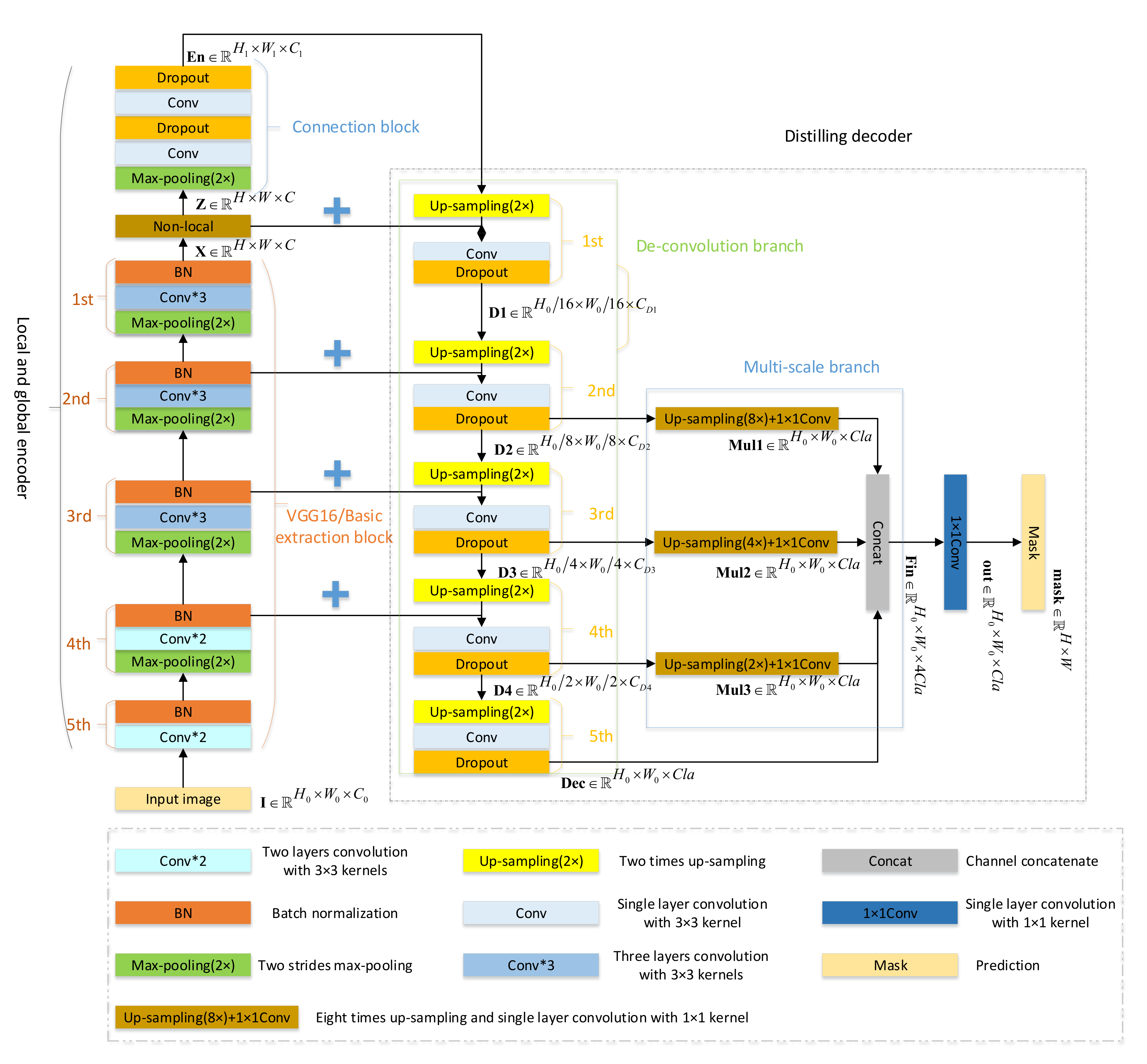
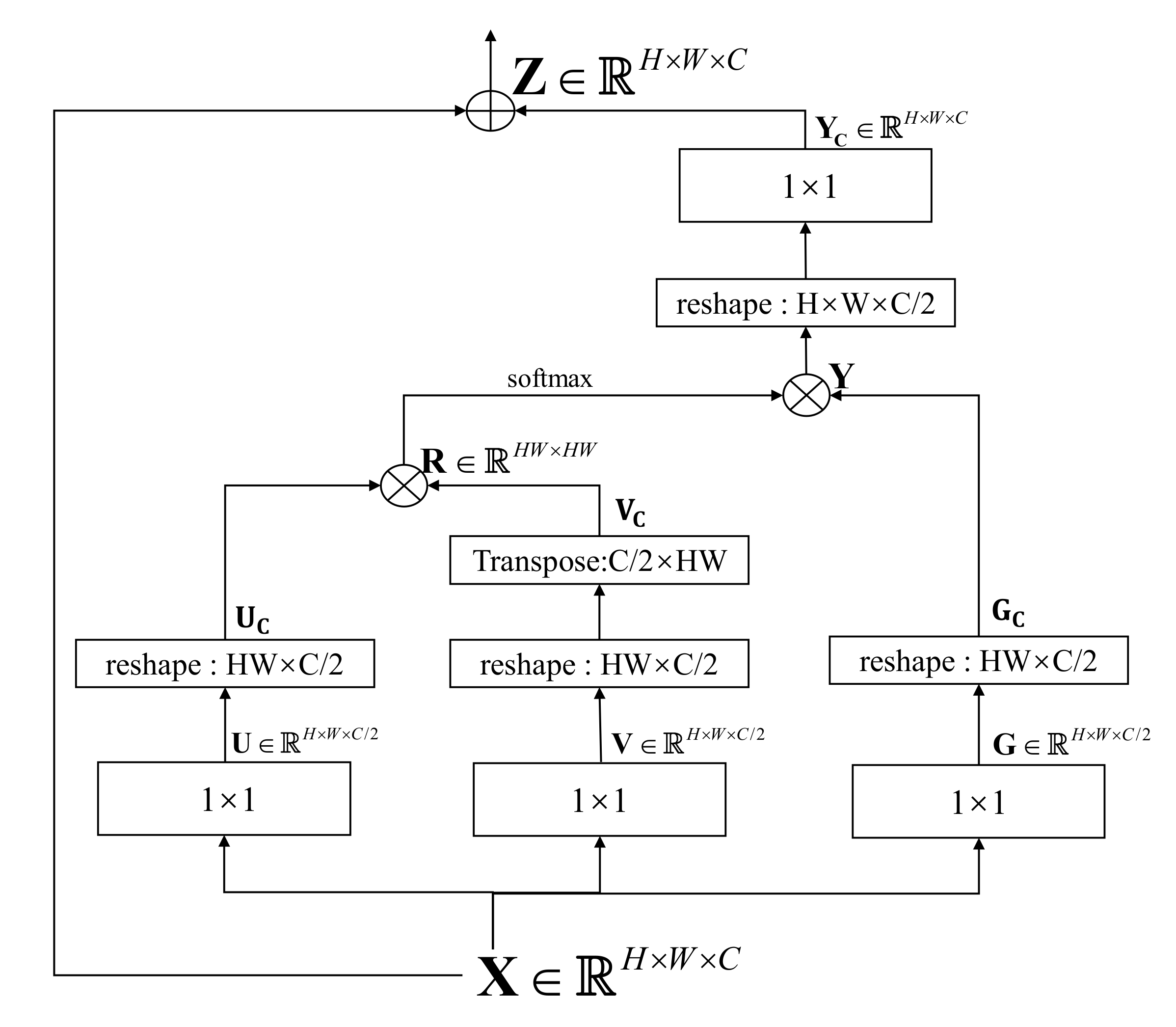
• The proposed GMEDN adopts the encoder-decoder framework with a simple skip connection scheme as the backbone. For the local and global encoder, a VGG16 is used to capture the local information from the aerial images. Based on this, the non-local block is introduced to explore the global information from the aerial images. Combing local and global information, the buildings with diverse shapes can be segmented.
• A distilling decoder is developed for our GMEDN, in which the de-convolution and the multi-scale branches are combined to explore the fundamental and multi-scale information from the aerial building images. Through the de-convolution branch, not only the low-level features (e.g., edge and texture) but also the high-level features (e.g., semantics) can be extracted from the images for segmenting the buildings. We name these features the fundamental information. By the multi-scale branch, the multi-scale information that is used to predict the buildings with different sizes can be captured. Integrating the fundamental and multi-scale information, the buildings with various sizes can be segmented.

The remaining of this paper is organized as follows. The related work of segmentation network and aerial building extraction are summarized in Section 2. In Section 3, we describe our GMEDN method in detail. Then the experimental and discussion are dedicated to Section 4. Finally, the conclusion of our letter is in Section 5.

2. Related Work

2.1. Semantic Segmentation Architecture

Image semantic segmentation is a classical problem in the computer vision community. With the development of deep learning, CNN becomes important in this topic. Here, we roughly divide the current deep CNN-based segmentation networks into three groups.

In the first group, the proposed methods are always general-purpose [30,31]. In 2015, the FCN model [27] transformed the fully connection layer of the traditional CNN into a series of convolutional layers. It provides a basic idea to solve semantic segmentation problem with the deep learning. Apart from FCN, another group of successful semantic segmentation networks were proposed and named DeepLab. There are three versions of DeepLab, and they were published in [32,33,34], respectively. DeepLab-v1 uses a fully connected conditional random field (CRF) at the end of the FCN framework to obtain more accurate information. To control the receptive field of the network, they adopt the dilated convolution to replace the last two pooling layers. Based on DeepLab-v1, DeepLab-v2 adds atrous spatial pyramid pooling (ASPP) into the network. ASPP contains dilated convolutions of different rates, which can capture the context of the image at multiple scales. Moreover, DeepLab-v2 uses deep residual network instead of VGG16 [29] (which was used in Deeplab-v1) to improve the performance of the model. Based on DeepLab-v2, DeepLab-v3 refines the structure of the network so that the segmentation results are further enhanced.

In the second group, researchers make full use of CNN’s hierarchical structure to extract rich information from the images, which is beneficial for segmenting complex contextual scenarios and small targets. For example, the pyramid scene parsing network (PSPNet) [35] aggregates the context information of different layers to improve the models’ capacity of obtaining global information. PSPNet embeds the multi-scale, global, and local information in the FCN-based framework through the pyramid structure. Furthermore, to speed up convergence, the authors add the supervisory loss function into the backbone network. Another popular method, feature pyramid network (FPN), was introduced in the literature [36]. It uses feature maps of different resolutions to explore objects of different sizes. Through continuous up-sampling and cross-layer fusion mechanism, both the low-level visual information and the high-level semantic information can be reflected by the output feature maps.

In the third group, scholars develop segmentation networks based on object detection algorithms. Inspired by the region selection idea, the mask region-based CNN (Mask R-CNN) was presented in the literature [37]. It adds the mask prediction branch on the basis of the structure of faster R-CNN [38] to complete the semantic segmentation. In addition, the regions of interest (RoI) Align is used to replace the RoI Pooling for removing the rough quantization. Although the segmentation performance of Mask R-CNN is positive, the evaluation function shared scheme would influence the segmentation results negatively. To address this issue, Huang et al. [39] developed the mask score R-CNN (MSR-CNN) model in 2019. It adds the Mask-IoU block to learn how to predict the quality of an instance mask and obtain a great result.

2.2. Aerial Building Extraction

The semantic segmentation methods discussed above are proposed for natural images. Although they can be used to complete the building extraction from the aerial images, their performance may not reach the satisfactory stage. Therefore, many aerial images oriented semantic segmentation approaches were introduced in recent years. Here, we review some popular aerial building extraction networks from the following two aspects.

The methods within the first group can be regarded as the variations of FCN. Based on FCN architecture, several post-processing technologies are developed to improve the performance of aerial building extraction. For example, in [40], the authors designed a patch-based CNN architecture. In the post-processing stage, they combine the low-level features of adjacent regions with CNN features to improve the performance. Shrestha et al. [41] proposed an enhanced FCN for building extraction. This model utilizes CRF to optimize the rough results obtained by the FCN for improving the performance of aerial building extraction. Another method was proposed in the literature [42], which is an end-to-end trainable gated residual refinement network (GRRNet). Through fusing the high-resolution aerial images and the LiDAR point clouds, GRRNet improves the performance of building extraction a lot.

Besides the FCN families, some other methods are developed with the consideration of the characteristics of the aerial images. To exactly extract the buildings from the aerial images, the high-quality features with multi-scale and detailed information are important. Therefore, some researchers pay their attention to feature learning. Yuan et al. [43] used a simple CNN to learn features and aggregated feature maps of multiple layers for the building prediction. Furthermore, the authors introduce the signed distance function to classify boundary pixels, which is useful to get fine segmentation results. In [44], another feature learning based building extraction method was proposed, which uses spatial residual inception (SRI) module to capture and aggregate multi-scale context information. This model could accurately identify large buildings while preserving global features and local detailed features. Besides the multi-scale schemes, there are some other approaches that can be used to obtain rich features for the semantic segmentation task. For example, Liu et al. [45] proposed their network with the encoder-decoder structure. By adding the skip connection, the information loss caused by the usual pooling could be reduced obviously. Furthermore, the spatial pyramid pooling is embedded in this model to ensure the rich contextual information can be learned. In [46], the authors combined the residual connection unit, the extended sensing unit, and the pyramid aggregation unit together to complete the building extraction task. Due to the introduction of the form filter, the boundaries of segmented results are accurate and smooth.

3. Methodology

3.1. Overall Framework

The pipeline of our building extraction model GMEDN is shown in Figure 1. It consists of a local and global encoder and a distilling decoder. For the local and global encoder, it is constructed by a basic feature extraction network (VGG16), a non-local block [47], and a connection block. It aims to explore the local and global information from the aerial images. Through mining the object-level and the spatial context information, the diverse and abundant buildings can be fully represented. The details of the local and global encoder are discussed in Section 3.2. For the distilling decoder, it contains the de-convolution branch and the multi-scale branch. The de-convolution branch captures the fundamental information (e.g., low-level visual features and the high-level semantics) and multi-scale branch explores multi-scale information, which are useful to segment accurately buildings with different sizes and distribution. The details of the distilling decoder are discussed in Section 3.3.

There is another point we want to touch on. As shown in Figure 1, there are five convolutional layers (i.e., convolution, max-pooling, and batch normalization) and five de-convolutional layers (i.e., up-sampling, convolution, and dropout) in the local and global encoder and the distilling decoder, respectively. Due to the max-pooling and the up-sampling operations, some information within the images and feature maps would be lost. To reduce this information loss, the output of the i-th convolutional layer and the output of the i-th de-convolutional layer are summed. The operation mentioned above is the simple skip connection, which is widespread in semantic segmentation networks [27,48,49].

3.2. Local and Global Encoder

Before introducing the local and global encoder, we describe the non-local block first. The non-local block [47] is developed to obtain global information by capturing the dependencies of all the pixels. The architecture of the non-local block is shown in Figure 2.

Suppose the input and the output feature maps of the non-local block are $\mathbf{X}\in {\mathbb{R}}^{H\times W\times C}$ and $\mathbf{Z}\in {\mathbb{R}}^{H\times W\times C}$, where H and W represent the height and width of the input feature maps, C indicates the number of the channels. First, the input $\mathbf{X}$ is convoluted by three groups of $1\times 1$ convolutions with different initialized weights to get the $\mathbf{U}\in {\mathbb{R}}^{H\times W\times C/2}$, $\mathbf{V}\in {\mathbb{R}}^{H\times W\times C/2}$, and $\mathbf{G}\in {\mathbb{R}}^{H\times W\times C/2}$. Note that, the $1\times 1$ convolution has two functions [50]. First, it can enhance the non-local block’s capacity of non-linear fitting due to the active function followed by the convolution. Second, it can change the input data’s channels through adjusting the numbers of kernels. Here, according to the literature [47], we set the numbers of $1\times 1$ convolution kernels within each group equal to $C/2$. Therefore, the sizes of the outputs ($\mathbf{U}$, $\mathbf{V}$, and $\mathbf{G}$) are $C/2$, which can be regarded as the channel reduction. Taking the $\mathbf{U}$ as an example, the process can be expressed as

$$\mathbf{U}(i,j)=(\mathbf{X}*\mathbf{K})(i,j)=\sum _m\sum _n\mathbf{x}(i+m,j+n)·\mathbf{k}(m,n)+\mathbf{b},$$

(1)

where $\mathbf{X}$ is the input feature maps, i and j are the coordinates of pixels of $\mathbf{X}$, $\mathbf{K}$ denotes the convolutional kernel, $\mathbf{k}(m,n)$ indicates the value of $\mathbf{K}$ in the coordinate $(m,n)$, $\mathbf{b}$ is the convolution bias, the sign “*” represents the convolution operation, and the sign “·” denotes the value multiplication.

Second, to use the similarity relationship between pixels for the complex contents mining, the non-local block constructs the similarity matrix $\mathbf{R}$ through $\mathbf{U}$ and $\mathbf{V}$, and further uses $\mathbf{R}$ to obtain global feature maps $\mathbf{Y}$. To obtain the affinity matrix $\mathbf{R}$, $\mathbf{U}$ and $\mathbf{V}$ are reshaped to ${\mathbf{U}}_{\mathbf{C}}\in {\mathbb{R}}^{HW\times C/2}$ and ${\mathbf{V}}_{\mathbf{C}}\in {\mathbb{R}}^{C/2\times HW}$ first. Then, $\mathbf{R}\in {\mathbb{R}}^{HW\times HW}$ is obtained by

$$\mathbf{R}={\mathbf{U}}_{\mathbf{C}}\times {\mathbf{V}}_{\mathbf{C}},$$

(2)

where $HW$ means the number of pixels, $C/2$ indicates the channels of each pixel, and the sign “×” represents the matrix multiplication. To get the global feature $\mathbf{Y}$, the similarity relationships between pixels are assigned as weights to the feature maps $\mathbf{G}$. Before that, a softmax is used to normalize the affinity matrix $\mathbf{R}$ and a reshape operation is adopted to transform $\mathbf{G}$ into ${\mathbf{G}}_{\mathbf{C}}\in {\mathbb{R}}^{HW\times C/2}$. The process of getting $\mathbf{Y}$ can be represented as the following equation,

$$\mathbf{Y}=softmax\left(\mathbf{R}\right)\times {\mathbf{G}}_{\mathbf{C}},$$

(3)

where the sign “×” denotes matrix multiplication.

Third, the output of the non-local block $\mathbf{Z}\in {\mathbb{R}}^{H\times W\times C}$ can be obtained by fusing the global feature $\mathbf{Y}$ and the input feature maps $\mathbf{X}$. This leads that $\mathbf{Z}$ contains not only the initial characteristics of single pixels but also the resemblance among all of the pixels. To complete the feature fusion, $\mathbf{Y}$ is transformed into ${\mathbf{Y}}_{\mathbf{C}}\in {\mathbb{R}}^{H\times W\times C}$ through the reshaping and $1\times 1$ convolution operations. This process can be expressed as

$$\mathbf{Z}=\mathbf{X}+{\mathbf{Y}}_{\mathbf{C}}.$$

(4)

The non-local block has several superiorities. First, since the number of channels is halved in the first step, the non-local block is a lightweight model that would not increase the computational cost to the original network. Second, since the input and output data have the same scale, the non-local block is a flexible model that can be embedded after any layer. In this paper, we put the non-local block on the top of the basic feature extraction network.

Based on the non-local block, we design our local and global encoder as follows. The local and global encoder is divided into three blocks, i.e., basic feature extraction network, non-local block, and connection block. First, we adopt VGG16 as the basic feature extraction network. VGG16 is a classical CNN, which contains five layers. The first, second, third layers consist of the same components, i.e., one max-pooling, three convolutions, and one batch normalization (BN) operations. The fourth layer contains two convolutions compared with the 1st layer. Then the 5th layer contains two convolutions and one batch normalization (BN) operations. The sizes of the kernels of the convolutions in VGG16 are $3\times 3$. The kernel sizes and the strides of max-pooling operations in VGG16 are $3\times 3$ and 2. Suppose the input image is $\mathbf{I}\in {\mathbb{R}}^{H_0\times W_0\times C_0}$, the output of VGG16 block can be represented by $\mathbf{X}\in {\mathbb{R}}^{H\times W\times C}$. Here the $H_0$, $W_0$, and $C_0$ represent the height, width, and a number of channels of the input image. This process can be expressed as

$$\mathbf{X}={\mathcal{F}}_{VGG16}(\mathbf{I},{\mathbf{W}}_{\mathbf{VGG}\mathbf{16}}),$$

(5)

where ${\mathcal{F}}_{VGG16}\left(·\right)$ denotes the mapping function of the VGG16 block and ${\mathbf{W}}_{\mathbf{VGG}\mathbf{16}}$ is the learnable weights of VGG16.

Second, we embed a non-local block on the top of VGG16 so that the input of the non-local block is $\mathbf{X}$. According to the above description of the non-local block, the output of the non-local block is $\mathbf{Z}\in {\mathbb{R}}^{H\times W\times C}$. This process can be expressed as

$$\mathbf{Z}={\mathcal{F}}_{non-local}(\mathbf{X},{\mathbf{W}}_{\mathbf{non}-\mathbf{local}}),$$

(6)

where ${\mathcal{F}}_{non-local}\left(·\right)$ denotes the mapping function of the non-local block and ${\mathbf{W}}_{\mathbf{non}-\mathbf{local}}$ represents the learnable weights of the non-local block. Since the non-local block can capture global information (e.g., buildings’ context within an aerial image), which can be used to distinguish the buildings from other objects. Thus, global information is beneficial to the building extraction task.

Third, we add a connection block on the top of the non-local block to fuse the information from VGG16 and non-local block. It contains a $3\times 3$ max-pooling with 2 strides and the repeated operations, i.e., $3\times 3$ convolution and dropout operations. Here, the convolution operation aims to fuse information through the weight matrix, the dropout operation is used to avoid overfitting. Suppose the input of connection block is $\mathbf{Z}\in {\mathbb{R}}^{H\times W\times C}$, the output can be represented by $\mathbf{En}\in {\mathbb{R}}^{H_1\times W_1\times C_1}$, where the $H_1$, $W_1$, and $C_1$ denote the height, width, and channels of the feature maps. The connection process can be expressed as

$$\mathbf{En}={\mathcal{F}}_{connection}(\mathbf{Z},{\mathbf{W}}_{\mathbf{connection}}),$$

(7)

where ${\mathcal{F}}_{connection}\left(·\right)$ denotes the mapping function of the connection block and ${\mathbf{W}}_{\mathbf{connection}}$ represents the learnable weights of the connection block.

3.3. Distilling Decoder

The distilling decoder is developed to obtain the final prediction mask which has the same size as the input image. There are two branches in the distilling decoder, i.e., a de-convolution branch and a multi-scale branch. In the de-convolution branch, there are five de-convolutional layers, constructed by 2 times up-sampling, $3\times 3$ convolution, and dropout operations. Here, the up-sampling and convolution operations are selected to accomplish the de-convolution operation. The dropout operation is adopted to prevent the issue of over-fitting. As shown in Figure 1, when $\mathbf{En}$ is input the de-convolution branch, the output of the 1st, 2nd, 3rd, and 4th layers are $\mathbf{D}\mathbf{1}\in {\mathbb{R}}^{H_0/16\times W_0/16\times C_{D1}}$, $\mathbf{D}\mathbf{2}\in {\mathbb{R}}^{H_0/8\times W_0/8\times C_{D2}}$, $\mathbf{D}\mathbf{3}\in {\mathbb{R}}^{H_0/4\times W_0/4\times C_{D3}}$, and $\mathbf{D}\mathbf{4}\in {\mathbb{R}}^{H_0/2\times W_0/2\times C_{D4}}$, respectively. Furthermore, the output of the de-convolution branch is $\mathbf{Dec}\in {\mathbb{R}}^{H_0\times W_0\times Cla}$, where $Cla$ denotes the number of classes. This process can be formulated as

$$\mathbf{Dec}={\mathcal{F}}_{de-convolution}(\mathbf{En},{\mathbf{W}}_{\mathbf{de}-\mathbf{convolution}}),$$

(8)

where the ${\mathcal{F}}_{de-convolution}\left(·\right)$ denotes the de-convolution branch and the ${\mathbf{W}}_{\mathbf{de}-\mathbf{convolution}}$ is the weights.

The output of the de-convolution branch $\mathbf{Dec}$ only contains fundamental information, which is limited to describe the buildings with diverse sizes accurately. Thus, the multi-scale branch is developed to fully explore the different scale information from the input aerial image. Here, the convolution and up-sampling operations are adopted to unify the sizes of outputs corresponding to the different de-convolutional layers. In detail, the 8, 4, and 2 times up-sampling are used for the feature maps $\mathbf{D}\mathbf{2}$, $\mathbf{D}\mathbf{3}$, $\mathbf{D}\mathbf{4}$, respectively. Meanwhile, the $1\times 1$ convolution is applied to reduce their dimensions to the number of classes. In this way, we get the following feature maps, i.e., $\mathbf{Mul}\mathbf{1}\in {\mathbb{R}}^{H_0\times W_0\times Cla}$, $\mathbf{Mul}\mathbf{2}\in {\mathbb{R}}^{H_0\times W_0\times Cla}$, and $\mathbf{Mul}\mathbf{3}\in {\mathbb{R}}^{H_0\times W_0\times Cla}$. Then, we concatenate them with $\mathbf{Dec}$ to get $\mathbf{Fin}\in {\mathbb{R}}^{H_0\times W_0\times 4Cla}$, which contains fundamental information and multi-scale information. This process is shown in the following equation

$$\begin{array}{c}\hfill \mathbf{Fin}=concat\left(\mathbf{Mul}\mathbf{1},\mathbf{Mul}\mathbf{2},\mathbf{Mul}\mathbf{3},\mathbf{Dec}\right),\end{array}$$

(9)

where the $concat\left(·\right)$ means that concatenates them on the channel. To reduce the channels of $\mathbf{Fin}\in {\mathbb{R}}^{H_0\times W_0\times 4Cla}$, we transform $\mathbf{Fin}\in {\mathbb{R}}^{H_0\times W_0\times 4Cla}$ to $\mathbf{out}\in {\mathbb{R}}^{H_0\times W_0\times Cla}$ through a $1\times 1$ convolution operation. Finally, a $\mathbf{mask}\in {\mathbb{R}}^{H_0\times W_0\times 1}$ with the values of semantic classes can be generated from $\mathbf{out}\in {\mathbb{R}}^{H_0\times W_0\times Cla}$ using the argmax function. In this paper, the mask is a binary prediction that denotes which pixel belongs to the building and which one to the background.

There are some points we should further explain. First, in our distilling decoder, the $3\times 3$ convolution is used to learn the features from the inputs, while the $1\times 1$ convolution is selected to reduce the number of dimensions through adjusting the number of convolutional kernels. Second, since the feature maps of the first de-convolutional layer have little high-level semantic information, we do not take them into account during the multi-scale fusion.

4. Experiments and Discussion

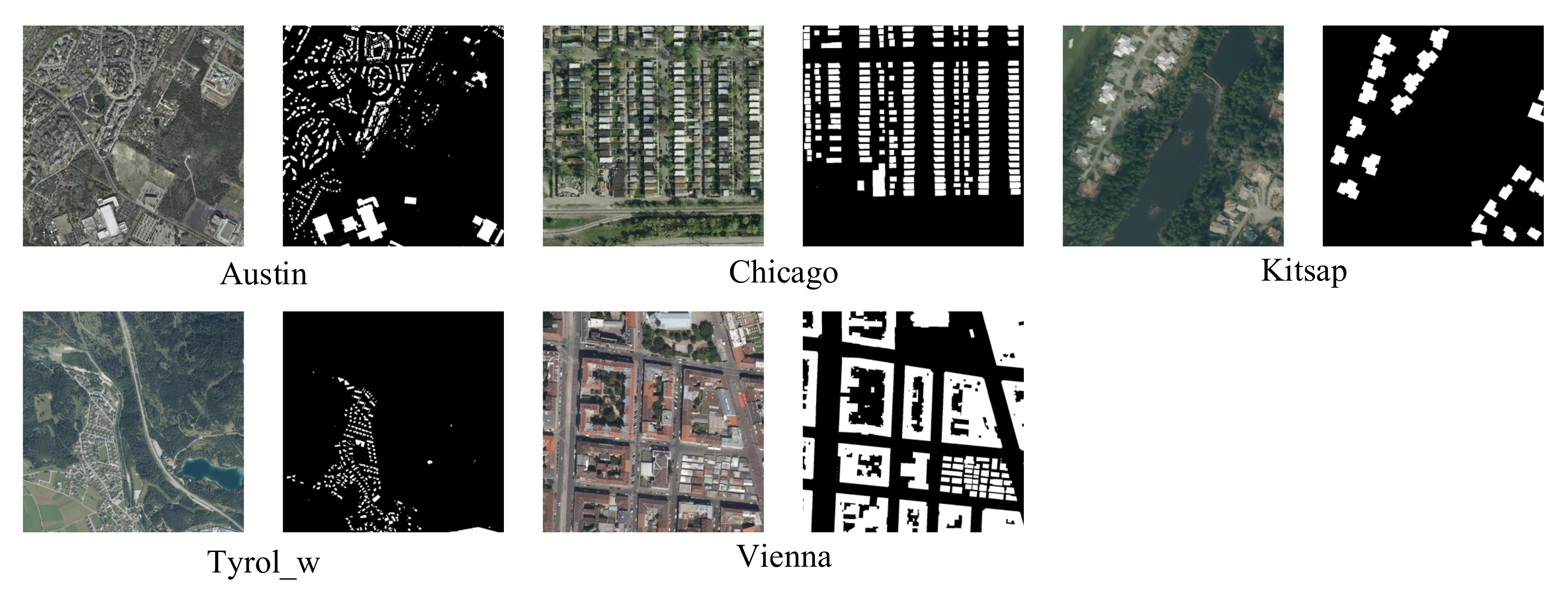
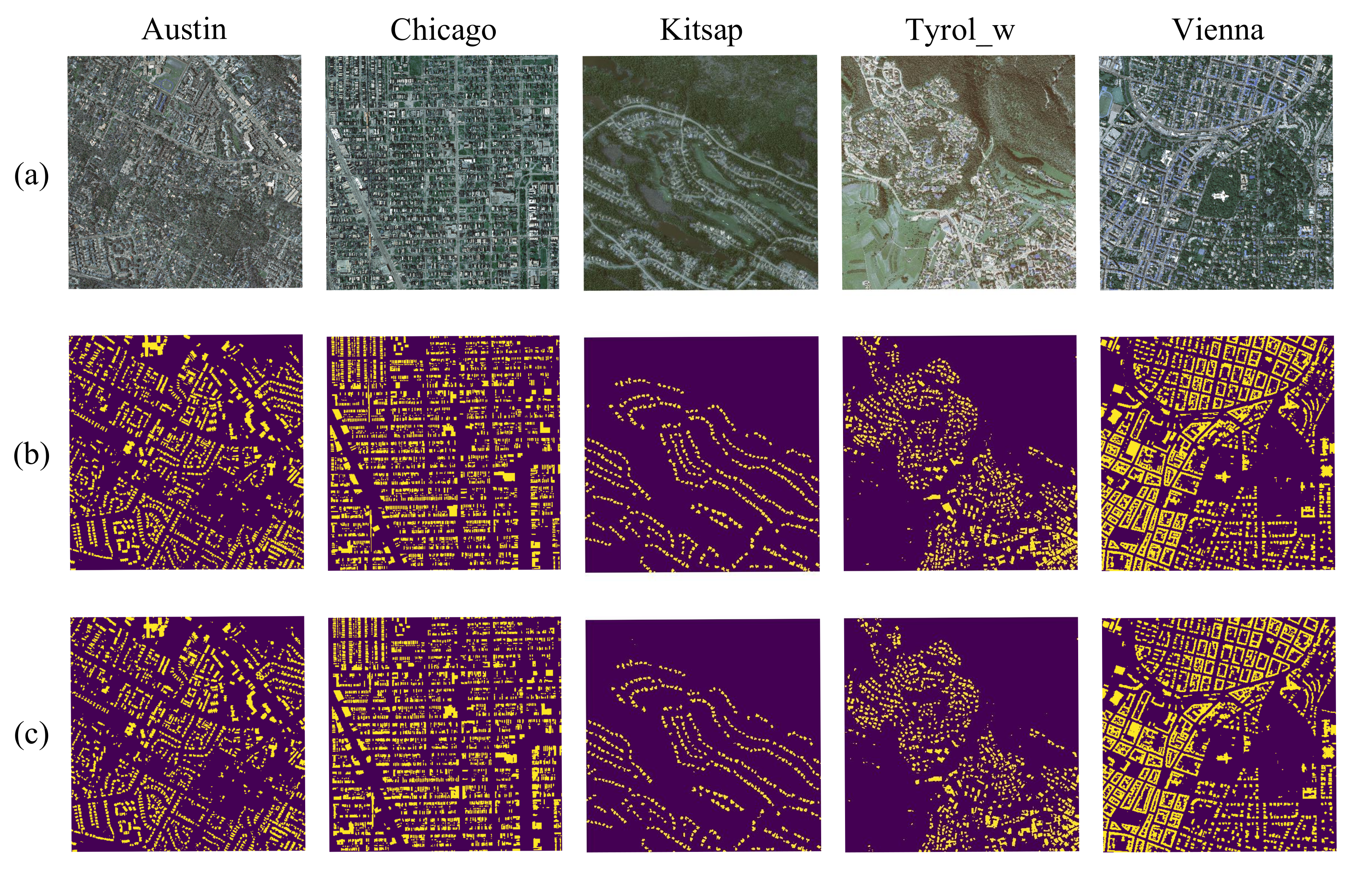
4.1. Datasets Introduction

In this paper, two benchmark datasets are chosen to verify our model, i.e., the Inria aerial image labeling dataset [1] and the Massachusetts building dataset [51]. Both of them have two classes, they are, building and non-building. The buildings in these datasets are diverse in type, various in volume, and different in distribution. Therefore, these two datasets are suitable to validate if our method is useful or not.

The Inria dataset contains 360 aerial Red-Green-Blue (RGB) images collected from ten cities and covers areas with 810 ${\mathrm{km}}^2$. Each city has 36 images, which are numbered 1 to 36. These images cover different urban settlements, from densely populated areas to sparsely populated forested towns. The sizes of these aerial images are $5000\times 5000$, and their spatial resolution is $0.3\mathrm{m}$. In this dataset, only 180 images (corresponding to five cities, i.e., Austin, Chicago, Kitsap, Western Tyrol, and Vienna) and their ground truth are published. Some examples, including images and their ground truth, are shown in Figure 3. Suggested by the authors who released this dataset [1], 31 images are selected randomly from each released city to construct the training set and the rest of the images are used to be the testing set in the following experiments.

The Massachusetts dataset consists of 151 aerial RGB images and corresponding semantic labels. This dataset is collected from the Boston area and covers roughly 340 ${\mathrm{km}}^2$. The size of each image is $1500\times 1500$ and the resolution is $1\mathrm{m}$. The whole dataset is randomly divided into a training set of 141 images and a testing set of 10 images. The types of buildings within this dataset are diverse, including individual houses, garages from urban and suburban areas, etc. Figure 4 exhibits two examples with their ground truth.

4.2. Experimental Settings

All of the experiments are carried out on an HP-Z840-Work station with Xeon (R) CPU E5-2630, GeForce GTX 1080, and 64 RAM. Our GMEDN is trained by the Adam optimizer with the sparse softmax cross-entropy loss function. Here, the parameters of Adam optimizer are set as follows, ${\beta }_1=0.9$, ${\beta }_2=0.999$, $ϵ=1\times {10}^{-8}$. In addition, we use a schedule decay of 0.004, a dropout rate of 0.5 and a small learning rate of $2\times {10}^{-4}$ to complete the training. We initialize the weights of the encoder (parts of VGG16) with pre-trained weights via ImageNet [52]. Other weights of our model are initialized with a Glorot uniform initializer that draws samples from a uniform distribution. The optimization is stopped at 40 epochs, and the early stopping scheme is adopted to avoid overfitting. Note that, due to the limitations of the GPU memory, original images are cropped into $256\times 256$ image patches in this paper. For the Inria dataset, the non-overlapped grid scheme is selected to generate the image patches. For the Massachusetts dataset, we use grids with a stride size of 156 to augment limited training patches.

To evaluate the effectiveness of our model numerically, two assessment criteria are selected, they are, overall accuracy (OA) and the intersection of union (IoU). OA is the ratio of the number of correctly predicted pixels to the total number of pixels in all test sets, which is defined as,

$$OA=\frac{N\left(\mathrm{correct}\_\mathrm{pixels}\right)}{N\left(\mathrm{total}\_\mathrm{pixels}\right)},$$

(10)

where $N\left(\mathrm{correct}\_\mathrm{pixels}\right)$ is the number of correctly predicted pixels, and $N\left(\mathrm{total}\_\mathrm{pixels}\right)$ is the number of the total number of testing pixels. IoU measures the correlation between prediction and target label, which is widely used in binary semantic segmentation tasks [6,53]. Here, IoU is defined as,

$$IoU(A,B)=\frac{area\left(A\cap B\right)}{area\left(A\cup B\right)},$$

(11)

where A is the prediction and B is the target label. IoU equals 0 means A and B do not overlap and 1 means that A and B are the same.

4.3. Performance of GMEDN

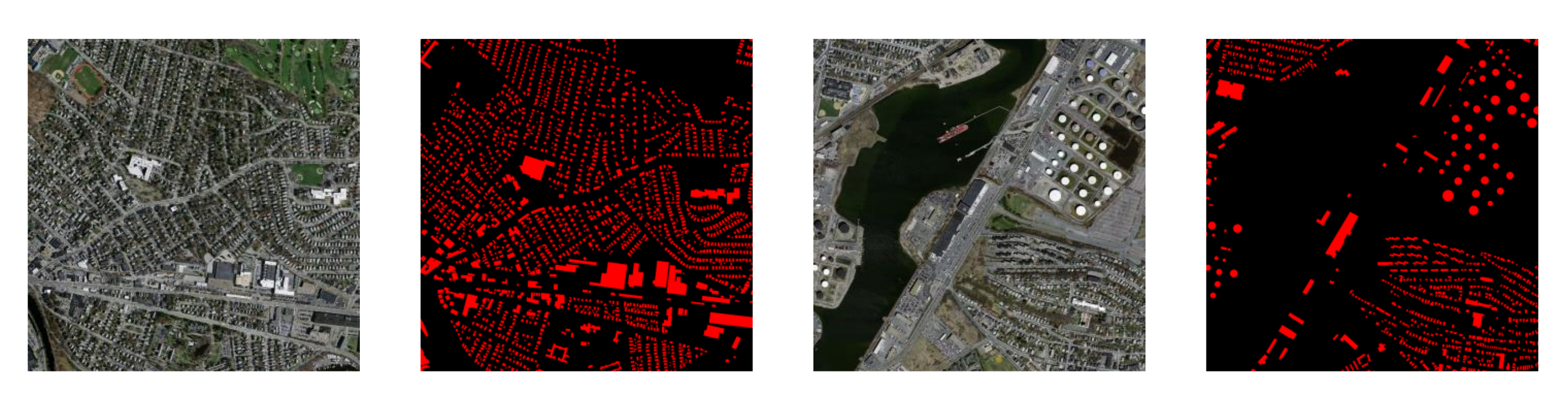
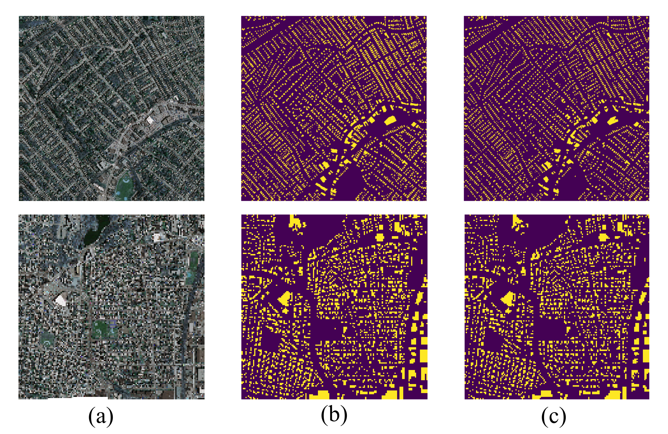
4.3.1. Building Extraction Examples

The building extraction results of our GMEDN model are exhibited and studied in this section.

For the Inria dataset, five images are selected from the published cities to accomplish the building extraction, and the results are exhibited in Figure 5. For each block, the original image, the ground truth map, and the results of our model are located in the top, middle, and bottom. From the observation of these images, we can find that our method can extract the diverse buildings positively. Taking the Chicago city as an example, although the buildings are dense in distribution and diverse in shape, our extraction result is similar to the ground truth map, in which the location of buildings is accurate and the boundaries of buildings are smooth. Taking the Kitsap city as another example, although the buildings are distributed sparsely and irregularly, our model can also obtain the promising extraction results compared with the ground truth. These encouraging results prove that our GMEDN is useful for the Inria dataset.

For the Massachusetts dataset, two images are chosen randomly to complete the building extraction by our model. The results are shown in Figure 6. As mentioned in Section 4.1, the resolution of these two images is $1\mathrm{m}$. Thus, compared with the images from the Inria dataset, the buildings within these aerial images are smaller in size but larger in volume, which increases the difficulty of extraction. Even so, through observing the extraction maps, we can easily find that the proposed method still achieves good performance. The buildings under the shadows of obstacles (such as trees, roads) are segmented well. These good visualization results indicate that our GMEDN is effective in the building extraction task.

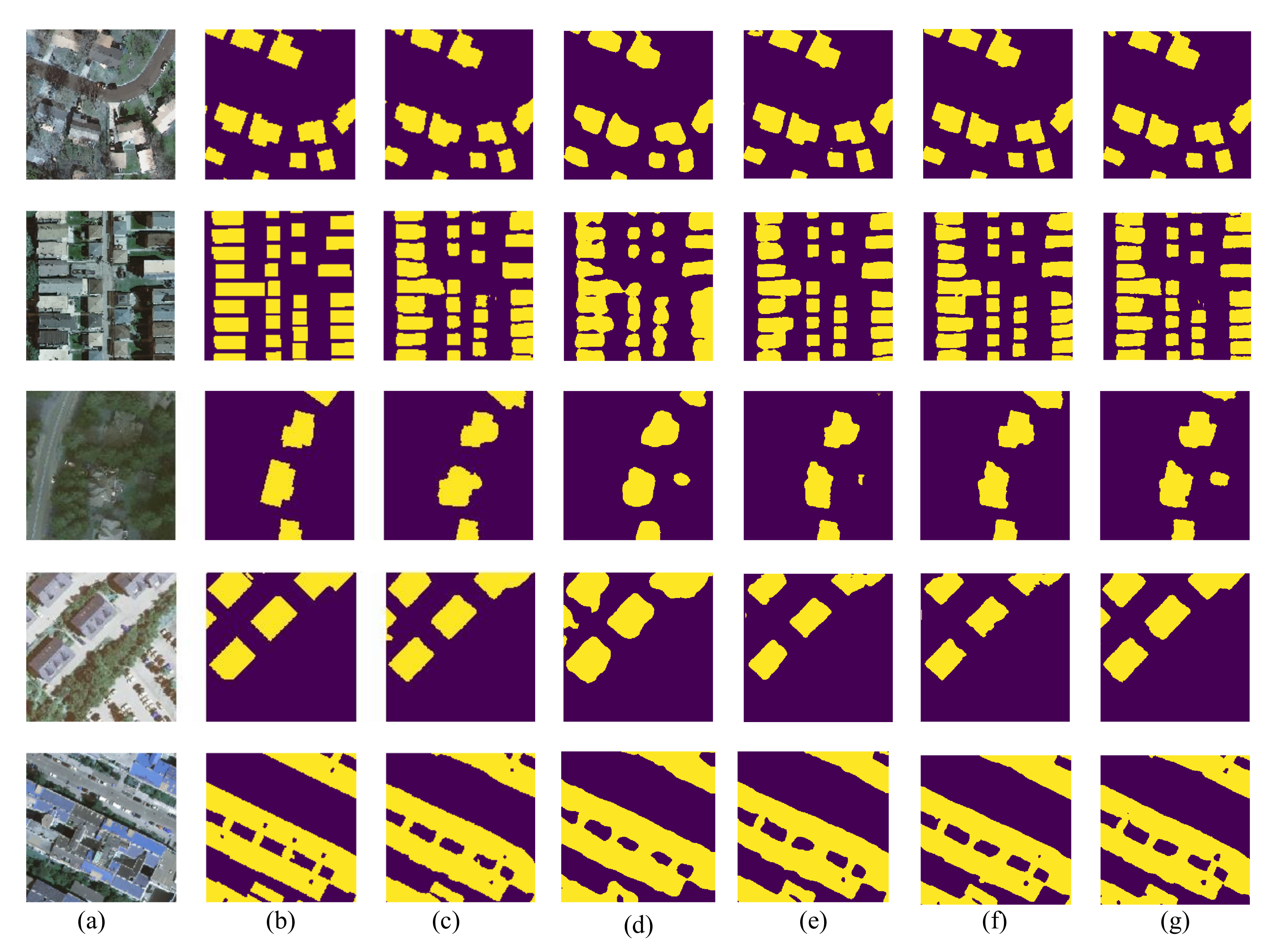
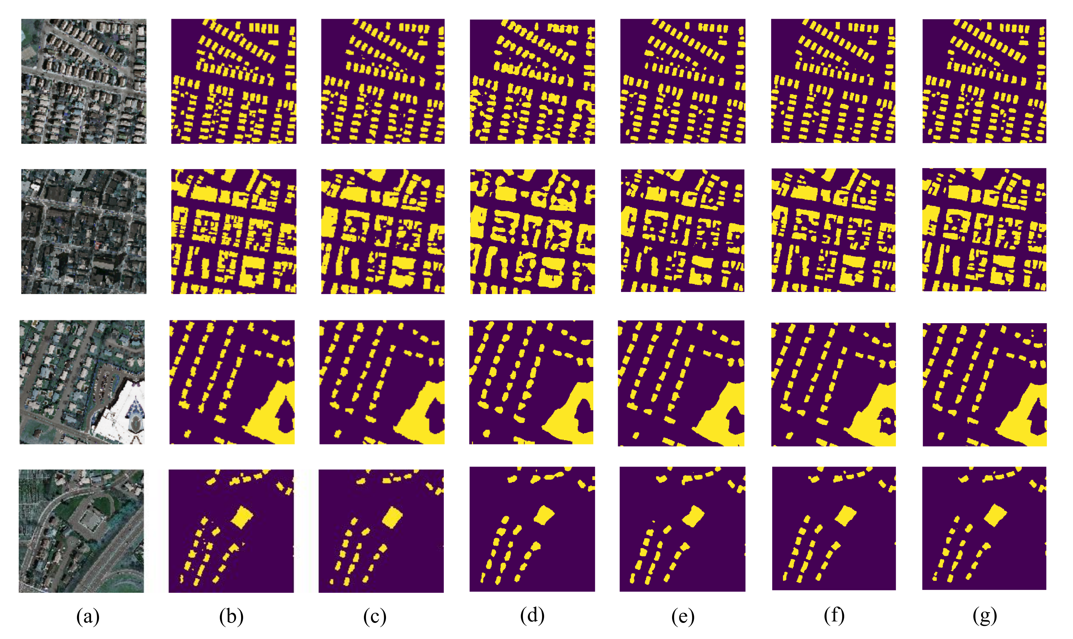
4.3.2. Comparisons with Different Methods

To further validate our method, we compare our GMEDN with the following four popular methods.

• Fully convolutional network (FCN). This may be the first general-purpose semantic segmentation network was proposed in 2015 [27]. The network consists of a common classification CNN (e.g., AlextNet [54] and VGG16 [29]) and several de-convolution layers. The CNN aims to learn the high-level features from the images while the deconvolution layers are used to predict the dense labels for pixels. Compared with the traditional methods, its cracking performance attracts scholars’ attention successfully.
• Deep convolutional segmentation network (SegNet). SegNet was introduced in the literature [55], which is an encoder-decoder model. SegNet first selects VGG16 as the encoder for extracting the semantic features. Then, a symmetrical network is established to be the decoder for transforming the low-resolution feature maps into the full input resolution maps and obtaining the segmentation results. Furthermore, a non-linear up-sampling scheme is developed to reduce the difficulty of the model training and generate the sparse decoder maps for the final prediction.
• U-Net with pyramid pooling layers (UNetPPL). The UNetPPL model was introduced in [56] for segmenting the buildings from high-resolution aerial images. By adding the pyramid pooling layers (PPL) in the U-Net [48], not only the shapes but also the global context information of the buildings can be explored, which ensures the segmentation performance.
• Symmetric fully convolutional network with discrete wavelet transform (FCNDWT). Taking the properties of aerial images into account, the FCNDWT model [49] fuses the deep features with the textural features to explore the objects from both spatial and spectral aspects. Furthermore, by introducing DWT into the network, FCNDWT is able to leverage the frequency information to analyze the images.

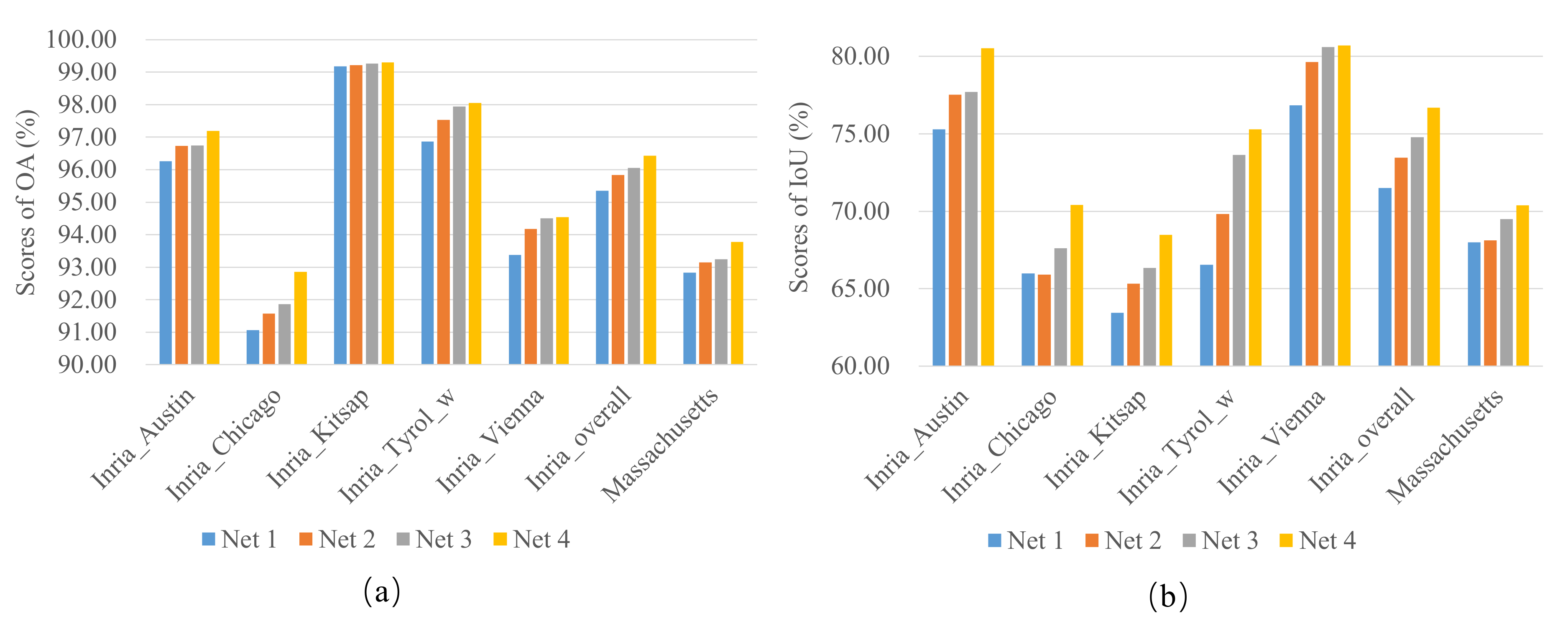
Note that, all of the comparisons are accomplished by ourselves, and their experimental settings are equal to ours for the sake of fairness.

The OA and IoU scores of different methods counted by the Inria dataset are displayed in

Table 1. IoU and OA scores of different methods counted by the Inria dataset (%).

	Methods	Austin	Chicago	Kitsap	Tyrol_w	Vienna	Overall
IoU	GMEDN	80.53	70.42	68.47	75.29	80.72	76.69
	FCN	76.44	67.28	66.05	71.25	75.43	72.33
	SegNet	78.46	68.37	60.29	59.61	78.37	72.83
	UNetPPL	80.04	67.40	64.83	61.61	78.87	73.33
	FCNDWT	78.34	69.99	65.41	73.19	79.70	75.30
OA	GMEDN	97.19	92.86	99.30	98.05	94.54	96.43
	FCN	96.56	91.90	99.24	97.44	93.01	95.63
	SegNet	96.84	92.28	99.15	96.73	93.76	95.75
	UNetPPL	97.13	91.96	99.23	97.00	93.90	95.84
	FCNDWT	96.85	92.70	99.22	97.86	94.26	96.17

. It is obvious that the proposed GMEDN performs best. Among all of the comparisons, the performance of FCN is the weakest. This is because that FCN is a general-purpose semantic segmentation model which does not consider the specific characteristics of aerial images. Compared with FCN, SegNet performs better since its sufficient de-convolution layers and the specific up-smapling scheme. Due to the multi-scale aggregation scheme, the behavior of UNetPPL is stronger than that of FCN and SegNet. However, its performance is still not as good as DWTFCN since the UNetPPL model does not take the textural features into account, which are beneficial to explore the objects from the complex background. Although the results obtained by the different compared methods are acceptable, our model outperforms others obviously. For the overall scenario, the proposed GMEDN achieves $76.69\%$ in IoU and $96.43\%$ in OA. Compared with other comparisons, the improvements in IoU created by our GMEDN are $4.36\%$ (FCN), $3.86\%$ (SegNet), $3.36\%$ (UNetPPL), and $1.39\%$ (FCNDWT). The enhancements in OA produced by our GMEDN are $0.8\%$ (FCN), $0.68\%$ (SegNet), $0.59\%$ (UNetPPL), and $0.26\%$ (FCNDWT). For the scenario of different cities, our method is still superior to other methods. Taking the Austin city as an example, the improvements in IoU/OA achieved by our model are $4.09\%/0.63\%$ (FCN), $2.07\%/0.35\%$ (SegNet), $0.49\%/0.06\%$ (UNetPPL), and $2.19\%/0.34\%$ (FCNDWT). These encouraging results demonstrate that our model is useful for the building extraction task.

The IoU and OA scores of different models counted by the Massachusetts dataset are summarized in

Table 2. IoU and OA scores of different methods counted by the Massachusetts dataset (%).

	GMEDN	FCN	SegNet	UNetPPL	FCNDWT
OA	93.78	92.66	92.56	92.98	93.30
IoU	70.39	66.50	63.43	65.65	67.96

. Similar to the Inria dataset’s results, our GMEDN still gets the best performance among all of the methods. The gains of our GMEDN in IoU/OA are $3.89\%/1.12\%$ (FCN), $6.96\%/1.22\%$ (SegNet), $4.74\%/0.8\%$ (UNetPPL), and $2.43\%/0.48\%$ (FCNDWT). Besides the above conclusion, a notable observation is that there is a distinct performance gap between GMEDN and other methods in IoU. The reasons behind this are summarized as follows. First, the details of buildings (e.g., shapes and edges) can be grasped by the backbone network. Second, through adding the non-local block, the global information can be further obtained which can be used to distinguish the objects from the complex background. Third, the multi-scale scheme can help our GMEDN model to capture the buildings with diverse sizes.

Apart from the numerical results, we also exhibit the building extraction results visually. Due to the space limitations, rather than showing the whole images’ results, the extraction results of the image patches with the size of $256\times 256$ are displayed. We select some image patches from the Inria dataset and the Massachusetts dataset randomly, and their building extraction masks are shown in Figure 7 and Figure 8.

Through observing those results, the following issues can be discovered. First, FCN and SegNet have smooth boundary prediction, and they perform well on the small buildings. Second, UNetPPL could extract more diverse buildings since the PPL model can learn the multi-scale information from aerial images. Third, FCNDWT achieves the good behavior on the building locations and boundaries as the intension frequency information is fused. Compared with the comparisons, the maps generated by our GMEDN have clear boundaries and precise locations. These positive visual extraction results prove the effectiveness of our method again.

4.4. Ablation Study

As mentioned in Section 3, GMEDN can be divided into four sub-models, including basic encoder-decoder network (i.e., VGG16, de-convolution branch, and skip connection), non-local block, connection block, and the multi-scale block. To study their contributions to the building extraction task, we design four networks to complete the building extraction respectively, they are,

• Net 1: Basic encoder-decoder network;
• Net 2: Basic encoder-decoder network + non-local block;
• Net 3: Basic encoder-decoder network + non-local block + connection block;
• Net 4: Basic encoder-decoder network + non-local block + connection block + multi-scale block.

Note that, the experimental settings of the networks in this section are the same as mentioned in Section 4.2.

The results of these networks counted on two datasets are shown in Figure 9, where Figure 9a shows the OA scores and Figure 9b displays the IoU scores. The first six groups of bars are the results of the Inria dataset and the last group of bars is the results of the Massachusetts dataset. From the observation of Figure 9, we can find the performance of different networks is proportional to the numbers of sub-models. In detail, the behavior of Net1 is the weakest among all compared networks since it only consists of a basic encoder-decoder network. After adding the non-local block, the performance of Net 2 is stronger than that of Net 1, which proves the usefulness of the non-local block. Due to the fusion scheme, Net 3 outperforms the Net 1 and Net 2 which confirms the contribution of the connection block. Integrating all sub-models, Net 4 achieves the best performance. Furthermore, the performance gap between Net 4 and other networks is distinct. The results discussed above demonstrate that each sub-model can make a positive contribution to our GMEDN model.

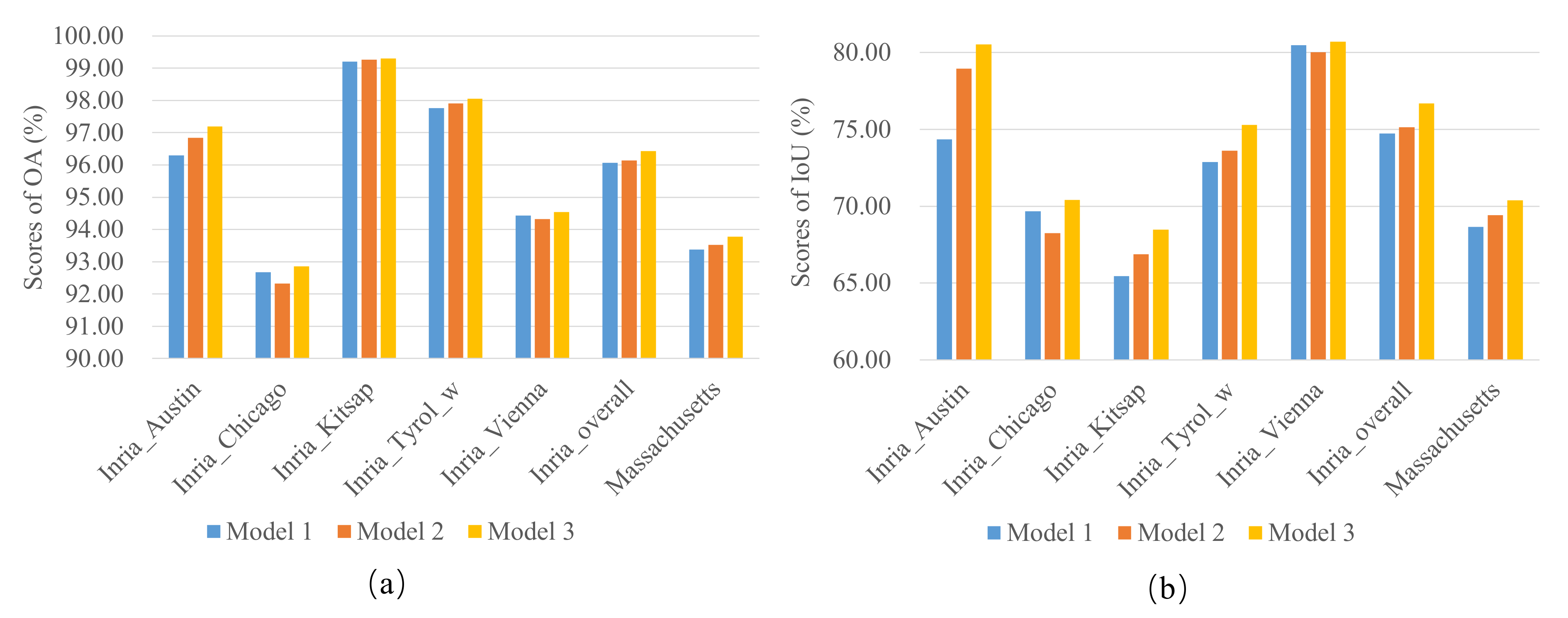
4.5. Robust Study of Non-Local Block

In this section, the robustness of the non-local block is studied. To this end, we vary the position of the non-local block. Here, to study the influence of the non-local block to GMEDN, we construct three models by changing the non-local block’s positions, i.e.,

• Model 1: Embedding the non-local block after the third layer of VGG16;
• Model 2: Embedding the non-local block after the fourth layer of VGG16;
• Model 3: Embedding the non-local block after the fifth layer of VGG16.

To get the segmentation results, three models are trained with the experimental settings discussed in Section 4.2. The OA and IoU scores counted on the Inria and Massachusetts datasets are exhibited in Figure 10, in which the first six sets of bars correspond to the Inria dataset while the last set of bars corresponds to the Massachusetts dataset. It is easy to find that the performance differences between the three models are small. Taking the Vienna city within the Inria dataset as an example, three models’ OA scores are $94.43\%$, $94.32\%$, and $94.54\%$, while their IoU scores are $80.47\%$, $80.02\%$, and $80.72\%$. This indicates that our GMEDN is not sensitive to the non-local block.

4.6. Running Time

Here, we discuss the time costs of our GEMDN from the training and inference aspects. As mentioned in Section 4.2, the input data is the $256\times 256$ aerial image patches that are cropped from the original aerial images. The volumes of the training sets are 1805 and 360 for the Inria and Massachusetts datasets. The training times of the two datasets are 5.71h and 5.23h, respectively. For the inference, the time cost of predicting one patch is 0.26s. Therefore, we need 98.7s to segment an aerial image ($5000\times 5000$) from the Inria dataset, and 9.36s to complete the building extraction from an aerial image ($1500\times 1500$) of the Massachusetts dataset.

5. Conclusions

With the consideration of the characteristics of aerial images, a simple yet useful method (GMEDN) is proposed in this paper for building extraction based on the encoder-decoder framework with a skip connection.

• To extract the local and global information from the aerial images for fully describing the buildings with various shapes, a local and global encoder is developed. It consists of a VGG16, a non-local block, and a connection block. VGG16 is used to learn the local information through several convolutional layers, the non-local block aims at learning global information from the similarities of all pixels, and the connection block further integrates local and global information.
• To explore the fundamental and multi-scale information from the aerial images for capturing the buildings with different sizes, a distilling decoder is developed. It contains a de-convolution branch and a multi-scale branch. The de-convolution branch focuses on learning the buildings’ representation (low- and high-level visual features) under different scales by several de-convolutional layers, and the multi-scale branch aims at fusing them to improve the discrimination of the prediction mask.
• To reduce the information loss caused by the max-pooling (encoder) and the up-sampling (decoder) operations, the simple skip connection is added between the local and global encoder and the distilling decoder.

The introduced GMEDN can accomplish the building extraction in an end-to-end manner, and its superiorities are confirmed by the encouraging experimental results counted on two aerial image datasets. Compared with some existing methods, for the Inria dataset, the minimum enhancements obtained by GMEDN are $0.26\%$ in and $1.39\%$ in IOU. For the Massachusetts dataset, the minimum gains achieved by GMEDN are $0.48\%$ in OA and $2.43\%$ in IOU.

Although GMEDN achieves positive results in building extraction tasks, it is not a lightweight network which limits its practicability in many realistic scenarios. To address this issue, we will pay our attention to developing the light model for the building extraction task in the future.

References

1. Maggiori, E.; Tarabalka, Y.; Charpiat, G.; Alliez, P. Can semantic labeling methods generalize to any city? The inria aerial image labeling benchmark. In Proceedings of the 2017 IEEE International Geoscience and Remote Sensing Symposium (IGARSS), Fort Worth, TX, USA, 23–28 July 2017; pp. 3226–3229. [Google Scholar]
2. Cheng, G.; Han, J.; Lu, X. Remote sensing image scene classification: Benchmark and state of the art. Proc. IEEE 2017, 105, 1865–1883. [Google Scholar] [CrossRef] [Green Version]
3. Marmanis, D.; Wegner, J.D.; Galliani, S.; Schindler, K.; Datcu, M.; Stilla, U. Semantic segmentation of aerial images with an ensemble of CNNs. ISPRS Ann. Photogramm. Remote Sens. Spat. Inf. Sci. 2016, 3, 473. [Google Scholar] [CrossRef] [Green Version]
4. Tang, X.; Liu, C.; Ma, J.; Zhang, X.; Liu, F.; Jiao, L. Large-Scale Remote Sensing Image Retrieval Based on Semi-Supervised Adversarial Hashing. Remote Sens. 2019, 11, 2055. [Google Scholar] [CrossRef] [Green Version]
5. Tang, X.; Zhang, X.; Liu, F.; Jiao, L. Unsupervised deep feature learning for remote sensing image retrieval. Remote Sens. 2018, 10, 1243. [Google Scholar] [CrossRef] [Green Version]
6. Mou, L.; Zhu, X.X. RiFCN: Recurrent network in fully convolutional network for semantic segmentation of high resolution remote sensing images. arXiv 2018, arXiv:1805.02091. [Google Scholar]
7. Zhang, X.; Ma, W.; Li, C.; Wu, J.; Tang, X.; Jiao, L. Fully Convolutional Network-Based Ensemble Method for Road Extraction From Aerial Images. IEEE Geosci. Remote Sens. Lett. 2019. [Google Scholar] [CrossRef]
8. Zhang, X.; Han, X.; Li, C.; Tang, X.; Zhou, H.; Jiao, L. Aerial image road extraction based on an improved generative adversarial network. Remote Sens. 2019, 11, 930. [Google Scholar] [CrossRef] [Green Version]
9. Ji, S.; Wei, S.; Lu, M. Fully convolutional networks for multisource building extraction from an open aerial and satellite imagery data set. IEEE Trans. Geosci. Remote Sens. 2018, 57, 574–586. [Google Scholar] [CrossRef]
10. Mou, L.; Zhu, X.X. Vehicle instance segmentation from aerial image and video using a multitask learning residual fully convolutional network. IEEE Trans. Geosci. Remote Sens. 2018, 56, 6699–6711. [Google Scholar] [CrossRef] [Green Version]
11. Shi, J.; Malik, J. Normalized cuts and image segmentation. IEEE Trans. Pattern Anal. Mach. Intell. 2000, 22, 888–905. [Google Scholar]
12. Rother, C.; Kolmogorov, V.; Blake, A. GrabCut: Interactive foreground extraction using iterated graph cuts. ACM Trans. Graph. (TOG) 2004, 23, 309–314. [Google Scholar] [CrossRef]
13. Shotton, J.; Johnson, M.; Cipolla, R. Semantic texton forests for image categorization and segmentation. In Proceedings of the 2008 IEEE Conference on Computer Vision and Pattern Recognition, Anchorage, AK, USA, 23–28 June 2008; pp. 1–8. [Google Scholar]
14. Vezhnevets, A.; Ferrari, V.; Buhmann, J.M. Weakly supervised semantic segmentation with a multi-image model. In Proceedings of the 2011 International Conference on Computer Vision, Barcelona, Spain, 6–13 November 2011; pp. 643–650. [Google Scholar]
15. Thoma, M. A survey of semantic segmentation. arXiv 2016, arXiv:1602.06541. [Google Scholar]
16. Li, A.; Bao, X. Extracting image dominant color features based on region growing. In Proceedings of the 2010 International Conference on Web Information Systems and Mining, Sanya, China, 23–24 October 2010; Volume 2, pp. 120–123. [Google Scholar]
17. Hong, Z.; Xuanbing, Z. Texture feature extraction based on wavelet transform. In Proceedings of the 2010 International Conference on Computer Application and System Modeling (ICCASM 2010), Taiyuan, China, 22–24 October 2010; Volume 14, pp. V14–V146. [Google Scholar]
18. Wang, J.; Xu, Z.; Liu, Y. Texture-based segmentation for extracting image shape features. In Proceedings of the 2013 19th International Conference on Automation and Computing, London, UK, 13–14 September 2013; pp. 1–6. [Google Scholar]
19. Cui, S.; Schwarz, G.; Datcu, M. Remote sensing image classification: No features, no clustering. IEEE J. Sel. Top. Appl. Earth Obs. Remote Sens. 2015, 8, 5158–5170. [Google Scholar] [CrossRef] [Green Version]
20. Hsu, C.W.; Lin, C.J. A comparison of methods for multiclass support vector machines. IEEE Trans. Neural Netw. 2002, 13, 415–425. [Google Scholar] [PubMed] [Green Version]
21. Safavian, S.R.; Landgrebe, D. A survey of decision tree classifier methodology. IEEE Trans. Syst. Man Cybern. 1991, 21, 660–674. [Google Scholar] [CrossRef] [Green Version]
22. Zhang, J.; Hong, X.; Guan, S.U.; Zhao, X.; Xin, H.; Xue, N. Maximum Gaussian mixture model for classification. In Proceedings of the 2016 8th International Conference on Information Technology in Medicine and Education (ITME), Fuzhou, China, 23–25 December 2016; pp. 587–591. [Google Scholar]
23. Kuang, P.; Cao, W.N.; Wu, Q. Preview on structures and algorithms of deep learning. In Proceedings of the 2014 11th International Computer Conference on Wavelet Actiev Media Technology and Information Processing (ICCWAMTIP), Chengdu, China, 19–21 December 2014; pp. 176–179. [Google Scholar]
24. Chen, X.; Xiang, S.; Liu, C.L.; Pan, C.H. Vehicle detection in satellite images by hybrid deep convolutional neural networks. IEEE Geosci. Remote Sens. Lett. 2014, 11, 1797–1801. [Google Scholar] [CrossRef]
25. Nguyen, K.; Fookes, C.; Sridharan, S. Improving deep convolutional neural networks with unsupervised feature learning. In Proceedings of the 2015 IEEE International Conference on Image Processing (ICIP), Quebec City, QC, Canada, 27–30 September 2015; pp. 2270–2274. [Google Scholar]
26. He, T.; Huang, W.; Qiao, Y.; Yao, J. Text-attentional convolutional neural network for scene text detection. IEEE Trans. Image Process. 2016, 25, 2529–2541. [Google Scholar] [CrossRef] [Green Version]
27. Long, J.; Shelhamer, E.; Darrell, T. Fully convolutional networks for semantic segmentation. In Proceedings of the IEEE Conference on Computer Vision and Pattern Recognition, Boston, MA, USA, 7–12 June 2015; pp. 3431–3440. [Google Scholar]
28. Wang, Y.; Chen, Q.; Zhu, Q.; Liu, L.; Li, C.; Zheng, D. A survey of mobile laser scanning applications and key techniques over urban areas. Remote Sens. 2019, 11, 1540. [Google Scholar] [CrossRef] [Green Version]
29. Simonyan, K.; Zisserman, A. Very deep convolutional networks for large-scale image recognition. arXiv 2014, arXiv:1409.1556. [Google Scholar]
30. Chen, L.C.; Zhu, Y.; Papandreou, G.; Schroff, F.; Adam, H. Encoder-decoder with atrous separable convolution for semantic image segmentation. In Proceedings of the European Conference on Computer Vision (ECCV), Munich, Germany, 8–14 September 2018; pp. 801–818. [Google Scholar]
31. Takikawa, T.; Acuna, D.; Jampani, V.; Fidler, S. Gated-scnn: Gated shape cnns for semantic segmentation. In Proceedings of the IEEE International Conference on Computer Vision, Seoul, Korea, 27 October–2 November 2019; pp. 5229–5238. [Google Scholar]
32. Chen, L.C.; Papandreou, G.; Kokkinos, I.; Murphy, K.; Yuille, A.L. Semantic image segmentation with deep convolutional nets and fully connected crfs. arXiv 2014, arXiv:1412.7062. [Google Scholar]
33. Chen, L.C.; Papandreou, G.; Kokkinos, I.; Murphy, K.; Yuille, A.L. Deeplab: Semantic image segmentation with deep convolutional nets, atrous convolution, and fully connected crfs. IEEE Trans. Pattern Anal. Mach. Intell. 2017, 40, 834–848. [Google Scholar] [CrossRef] [PubMed]
34. Chen, L.C.; Papandreou, G.; Schroff, F.; Adam, H. Rethinking atrous convolution for semantic image segmentation. arXiv 2017, arXiv:1706.05587. [Google Scholar]
35. Zhao, H.; Shi, J.; Qi, X.; Wang, X.; Jia, J. Pyramid scene parsing network. In Proceedings of the IEEE Conference on Computer Vision and Pattern Recognition, Honolulu, HI, USA, 21–26 July 2017; pp. 2881–2890. [Google Scholar]
36. Lin, T.Y.; Dollár, P.; Girshick, R.; He, K.; Hariharan, B.; Belongie, S. Feature pyramid networks for object detection. In Proceedings of the IEEE Conference on Computer Vision and Pattern Recognition, Honolulu, HI, USA, 21–26 July 2017; pp. 2117–2125. [Google Scholar]
37. He, K.; Gkioxari, G.; Dollár, P.; Girshick, R. Mask r-cnn. In Proceedings of the IEEE International Conference on Computer Vision, Venice, Italy, 22–29 October 2017; pp. 2961–2969. [Google Scholar]
38. Ren, S.; He, K.; Girshick, R.; Sun, J. Faster r-cnn: Towards real-time object detection with region proposal networks. In Proceedings of the Advances in Neural Information Processing Systems, Montreal, QC, Canada, 7–12 December 2015; pp. 91–99. [Google Scholar]
39. Huang, Z.; Huang, L.; Gong, Y.; Huang, C.; Wang, X. Mask scoring r-cnn. In Proceedings of the IEEE Conference on Computer Vision and Pattern Recognition, Long Beach, CA, USA, 16–20 June 2019; pp. 6409–6418. [Google Scholar]
40. Alshehhi, R.; Marpu, P.R.; Woon, W.L.; Dalla Mura, M. Simultaneous extraction of roads and buildings in remote sensing imagery with convolutional neural networks. ISPRS J. Photogramm. Remote Sens. 2017, 130, 139–149. [Google Scholar] [CrossRef]
41. Shrestha, S.; Vanneschi, L. Improved fully convolutional network with conditional random fields for building extraction. Remote Sens. 2018, 10, 1135. [Google Scholar] [CrossRef] [Green Version]
42. Huang, J.; Zhang, X.; Xin, Q.; Sun, Y.; Zhang, P. Automatic building extraction from high-resolution aerial images and LiDAR data using gated residual refinement network. ISPRS J. Photogramm. Remote Sens. 2019, 151, 91–105. [Google Scholar] [CrossRef]
43. Yuan, J. Learning building extraction in aerial scenes with convolutional networks. IEEE Trans. Pattern Anal. Mach. Intell. 2017, 40, 2793–2798. [Google Scholar] [CrossRef]
44. Liu, P.; Liu, X.; Liu, M.; Shi, Q.; Yang, J.; Xu, X.; Zhang, Y. Building footprint extraction from high-resolution images via spatial residual inception convolutional neural network. Remote Sens. 2019, 11, 830. [Google Scholar] [CrossRef] [Green Version]
45. Liu, Y.; Gross, L.; Li, Z.; Li, X.; Fan, X.; Qi, W. Automatic building extraction on high-resolution remote sensing imagery using deep convolutional encoder-decoder with spatial pyramid pooling. IEEE Access 2019, 7, 128774–128786. [Google Scholar] [CrossRef]
46. Xie, Y.; Zhu, J.; Cao, Y.; Feng, D.; Hu, M.; Li, W.; Zhang, Y.; Fu, L. Refined Extraction of Building Outlines from High-resolution Remote Sensing Imagery Based on a Multifeature Convolutional Neural Network and Morphological Filtering. IEEE J. Sel. Top. Appl. Earth Obs. Remote Sens. 2020, 13, 1842–1855. [Google Scholar] [CrossRef]
47. Wang, X.; Girshick, R.; Gupta, A.; He, K. Non-local neural networks. In Proceedings of the IEEE Conference on Computer Vision and Pattern Recognition, Salt Lake City, UT, USA, 18–23 June 2018; pp. 7794–7803. [Google Scholar]
48. Ronneberger, O.; Fischer, P.; Brox, T. U-net: Convolutional networks for biomedical image segmentation. In Medical Image Computing and Computer-Assisted Intervention—MICCAI 2015; Springer: Cham, Swizerland, 2015; pp. 234–241. [Google Scholar]
49. Azimi, S.M.; Fischer, P.; Körner, M.; Reinartz, P. Aerial LaneNet: Lane-marking semantic segmentation in aerial imagery using wavelet-enhanced cost-sensitive symmetric fully convolutional neural networks. IEEE Trans. Geosci. Remote Sens. 2018, 57, 2920–2938. [Google Scholar] [CrossRef] [Green Version]
50. Lin, M.; Chen, Q.; Yan, S. Network in network. arXiv 2013, arXiv:1312.4400. [Google Scholar]
51. Mnih, V. Machine Learning for Aerial Image Labeling; University of Toronto: Toronto, ON, Canada, 2013. [Google Scholar]
52. Russakovsky, O.; Deng, J.; Su, H.; Krause, J.; Satheesh, S.; Ma, S.; Huang, Z.; Karpathy, A.; Khosla, A.; Bernstein, M.; et al. Imagenet large scale visual recognition challenge. Int. J. Comput. Vis. 2015, 115, 211–252. [Google Scholar] [CrossRef] [Green Version]
53. Singh, P.; Komodakis, N. Effective Building Extraction by Learning to Detect and Correct Erroneous Labels in Segmentation Mask. In Proceedings of the IGARSS 2018—2018 IEEE International Geoscience and Remote Sensing Symposium, Valencia, Spain, 22–27 July 2018; pp. 1288–1291. [Google Scholar]
54. Krizhevsky, A.; Sutskever, I.; Hinton, G.E. Imagenet classification with deep convolutional neural networks. In Proceedings of the Advances in Neural Information Processing Systems, Lake Tahoe, NV, USA, 3–8 December 2012; pp. 1097–1105. [Google Scholar]
55. Badrinarayanan, V.; Kendall, A.; Cipolla, R. Segnet: A deep convolutional encoder-decoder architecture for image segmentation. IEEE Trans. Pattern Anal. Mach. Intell. 2017, 39, 2481–2495. [Google Scholar] [CrossRef] [PubMed]
56. Kim, J.H.; Lee, H.; Hong, S.J.; Kim, S.; Park, J.; Hwang, J.Y.; Choi, J.P. Objects segmentation from high-resolution aerial images using U-Net with pyramid pooling layers. IEEE Geosci. Remote Sens. Lett. 2018, 16, 115–119. [Google Scholar] [CrossRef]
Figure 1. Framework of our global multi-scale encoder-decoder network (GMEDN).
Remotesensing 12 02350 g001
Figure 2. Framework of our non-local block.
Remotesensing 12 02350 g002
Figure 3. Examples and their ground truth of the Inria dataset. Left: Image, Right: Ground truth.
Remotesensing 12 02350 g003
Figure 4. Examples and their ground truth of the Massachusetts dataset. Left: Image, Right: Ground truth.
Remotesensing 12 02350 g004
Figure 5. Building extraction results of our GMEDN model. Five images are randomly selected from the Inria dataset. They belong to Austin, Chicago, Kitsap, Tyrol_w, and Vienna cities respectively. (a) Original image, (b) Ground truth, (c) Prediction.
Remotesensing 12 02350 g005
Figure 6. Building extraction results of our GMEDN model. Two images are randomly selected from the Massachusetts dataset. (a) Original image, (b) Ground truth, (c) Prediction.
Remotesensing 12 02350 g006
Figure 7. Predictions of some patches of different methods on the Inria dataset. (a) Original image, (b) Ground truth, (c) GMEDN, (d) FCN, (e) SegNet, (f) UNetPPL, (g) FCNDWT.
Remotesensing 12 02350 g007
Figure 8. Predictions of some patches of different methods on the Massachusetts dataset. (a) Original image, (b) Ground truth, (c) GMEDN, (d) FCN, (e) SegNet, (f) UNetPPL, (g) FCNDWT.
Remotesensing 12 02350 g008
Figure 9. Ablation study of our GMEDN. (a) Results in OA, (b) Results in IoU.
Remotesensing 12 02350 g009
Figure 10. Robust study of non-local block. (a) Results in OA, (b) Results in IoU.
Remotesensing 12 02350 g010