A Non-Local Low-Rank Algorithm for Sub-Bottom Profile Sonar Image Denoising

Abstract

Due to the influence of equipment instability and surveying environment, scattering echoes and other factors, it is sometimes difficult to obtain high-quality sub-bottom profile (SBP) images by traditional denoising methods. In this paper, a novel SBP image denoising method is developed for obtaining underlying clean images based on a non-local low-rank framework. Firstly, to take advantage of the inherent layering structures of the SBP image, a direction image is obtained and used as a guidance image. Secondly, the robust guidance weight for accurately selecting the similar patches is given. A novel denoising method combining the weight and a non-local low-rank filtering framework is proposed. Thirdly, after discussing the filtering parameter settings, the proposed method is tested in actual measurements of sub-bottom, both in deep water and shallow water. Experimental results validate the excellent performance of the proposed method. Finally, the proposed method is verified and compared with other methods quantificationally based on the synthetic images and has achieved the total average peak signal-to-noise ratio (PSNR) of 21.77 and structural similarity index (SSIM) of 0.573, which is far better than other methods.

1. Introduction

As an important role in underwater tasks, sonar equipment has been widely used in marine geological survey, underwater engineering, and target detection for a long time [1,2,3,4]. Sub-bottom profiler (SBP), as one of the most important sonar equipment, provides information which is extensively used to determine sediment layering structures and physical properties in underwater acoustics applications [5]. However, the instability of equipment, marine environmental noise, as well as scattering echoes, degrade the quality of the SBP image, which limits the application of the SBP image [5,6]. Few researchers have paid attention to the SBP image denoising. In most cases, seriously polluted SBP images will be abandoned, since noise can greatly reduce the accuracy of horizon picking and adversely affect subsequent tasks such as interpretations. Low-level noise-polluted SBP images will still be used, but the interpretation efficiency will be decreased. With the development of ocean exploitation, poor-quality data cannot satisfy the demands of marine science research and ocean engineer applications. Thus, improving SBP image quality becomes important.

Though few researchers have studied SBP image denoising, there is a lot of research studying denoising algorithms based on optical images, ultrasound images, and side-scan sonar (SSS) images. Reviewing their works is helpful for our task.

Non-local Means (NLM) filtering, proposed by Buades et al. [7] in 2005, was the first method taking the non-local self-similarity of the image into consideration. The Block-Matching and three-dimensional (3D) filtering (BM3D) method [8] proposed by Dabov et al. in 2007 combined the transform-domain algorithm with the non-local spatial information, achieving great denoising performance by sparse 3D transform-domain collaborative filtering. Dong et al. [9] proposed a local and non-local sparsity-based image denoising method via dictionary learning and structural clustering and named their method clustering-based sparse representation (CSR). Zuo et al. [10] modified CSR via gradient histogram preservation. Their methods all achieved great success. It can be concluded that the successes of these state-of-the-art image denoising algorithms are based on the exploitation of image non-local self-similarity in some degree. Further, by vectoring all non-local similar patches as column vectors and stacking them as a matrix, a matrix with low-rank structure can be obtained [11]. Considering the low-rank characteristic, several researchers proposed non-local low-rank filtering methods. For example, Zhu et al. [12] proposed a non-local low-rank framework for ultrasound speckle reduction and Xie et al. [13] proposed a 3D tensor based on the non-local low-rank method to denoise positron emission tomography. Their works improved the noise filtering performances and preserved the fine details of the image.

Nowadays, denoising methods based on SSS images have also made great progress. Shang et al. [14] proposed a multi-resolution analysis method in sonar image denoising by adopting the finite Ridgelet transform to effectively resolve the line singularity, and a good performance in edge preserving has been achieved. Ioana et al. [15] presented an effective image denoising algorithm for SSS images using a variant of hyper-analytic wavelet transform. Both of their methods applied the transform-domain algorithm. Usually, transforms can achieve good sparsity for spatial details like edges and singularities [14]. Apart from transform-domain denoising methods, non-local denoising methods also attracted a lot of attention. Wang et al. [16] adopted the non-local spatial information to reduce noise and used the golden ratio to determine the denoising parameters. Owing to non-local spatial constraint, the performance of their method is good. Jin et al. [17] proposed a non-local structural sparsity-based image denoising algorithm to remove non-homogeneous noise from SSS images. The main contribution of their work is that they took some texture features into account, such as pixel intensity and Local Binary Pattern (LBP), to reinforce traditional CSR denoising models.

Though there have been a lot of achievements by the researchers above, there are several points worth noting when considering the denoising on a SBP image. Firstly, sonar images are always polluted by scattered echoes. For example, scattered echoes on rough seabed surface can produce speckle noise on a SSS image. As for SBP images, scattered echoes on sediment interfaces beneath the seabed can also produce speckle noise. Secondly, the volume scattering caused by the interior of sediment also degrades the SBP image quality. Then, the noise on the SBP image is more complex than that of a SSS image.

Since the non-local low-rank filtering framework has been proven to be effective, we adopt it in this paper. However, stronger noise produced by scattered echoes on SBP images compared with that on SSS images may have a negative impact on the non-local patch selection during filtering. To overcome this problem, in this paper, we propose a non-local low-rank denoising method with the constraint of guidance image. The proposed method firstly uses the vessel enhancement filtering to obtain the direction image and uses it as the guidance image, then calculates the guidance weight based on the guidance image. Guidance weight is derived from the guidance image and can ensure accurate patch selection compared with the conventional approaches. The remainder of this paper is organized as follows: Section 2 describes the denoising method in detail, Section 3 designs the experiments to verify the proposed method and analyzes the results, and Section 4 and Section 5 present the discussions and conclusions based on the experiments.

2. Method

2.1. The Non-Local Low-Rank Framework

Non-local methods such as NLM use non-local information by searching similar patches in a larger neighborhood of a reference patch. As shown in Figure 1a, the red rectangle is the reference patch, and the other rectangles are the searching patches. Different colors of the rectangles denote different similarities between the reference patch and the searching patches. Patches having a similar structure to the reference patch are assigned high weights, and vice versa. After getting all these similar patches, a patch group is constructed, as shown in Figure 1b. Every patch can be rearranged as a column of data. Then, the patch group can be rearranged as a matrix with low-rank structure. Figure 1b,c show the procedure of the rearrangement.

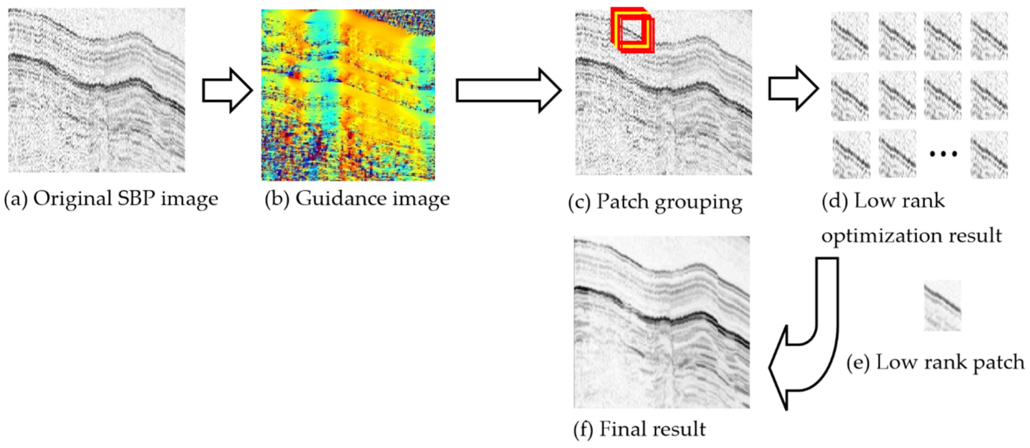
A guidance image is obtained at first. Then, guidance weight is calculated based on the guidance image, and similar patches are selected with the guidance weight constraint. After that, patch groups are constructed and used to construct a low-rank matrix. Finally, a low-rank approximation model is applied to the low-rank matrix to tackle the problem of image denoising, and a clean image can be obtained. Figure 2 provides an overview of the proposed filtering method. The proposed method begins by computing a guidance image and guidance weight to improve the robustness of the selection of similar patches.

2.2. Guidance Image

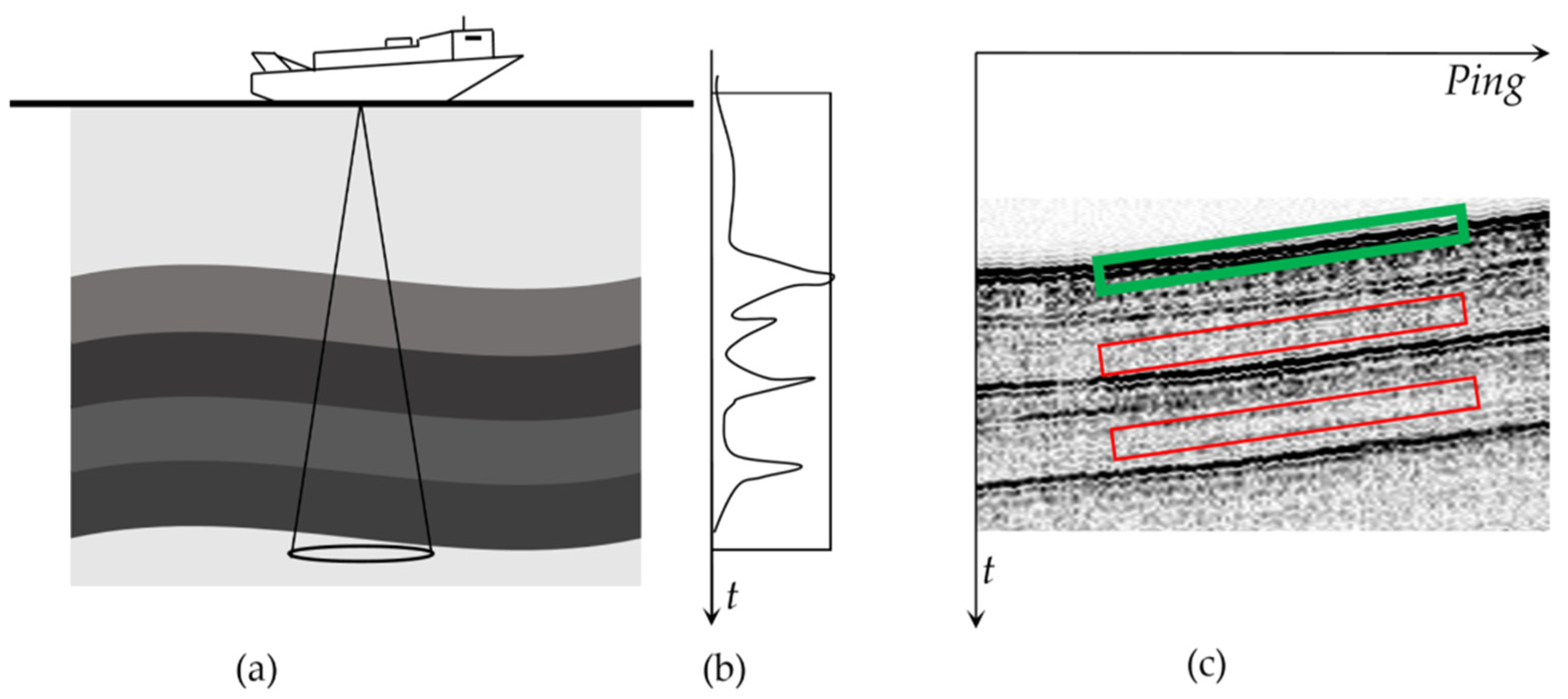
As shown in Figure 3a, sub-bottom profiler receives echoes coming from the reflections on the interfaces between adjacent sediments [18]. Figure 3b shows the received SBP echoes, sediment interface is displayed as a line-like structure in Figure 3c (marked with a green rectangle). The line-like structure can be considered as the inherent characteristic of sediment interface on the SBP image and is a significant characteristic that we can make full use of to help select the correct similar non-local patches.

In fact, due to the strong noise, directly applying the conventional Euclidean distance used in NLM is not always effective. In other image denoising fields, such as Magnetic Resonance Imaging (MRI) and ultrasound image denoising, it has been proven that a guidance image can be helpful in the selection of a non-local patch [12,19]. The key is to find an appropriate method to generate the guidance image for denoising. Since the line-like layer structures on SBP images can be distinguished from noise [20], we adopt the vessel enhancement filtering firstly, which can enhance line-like structures and suppress noise.

The enhanced image of original SBP image IM_original (IM_original is invert-colored) can be constructed as:

$$if \begin{array}{c}{\lambda }_2>0 \\ {\lambda }_2\le 0 \end{array} then \begin{array}{c}IM\left({\sigma }_0\right)=0\\ IM\left({\sigma }_0\right)=\exp \left(-\frac{R_B^2}{2{\beta }^2}\right)\left(1-\exp \left(-\frac{S^2}{2c^2}\right)\right)\end{array}$$

(1)

$$R_B=\frac{{\lambda }_1}{{\lambda }_2}, S=\sqrt{{\lambda }_1^2+{\lambda }_2^2}$$

(2)

where IM(σ₀) is the enhanced result, and ${\mathsf{\lambda }}_1$ and ${\mathsf{\lambda }}_2$ in Equation (1) represent the eigenvalues of the Hessian matrix (${\mathsf{\lambda }}_2\ge {\mathsf{\lambda }}_1$). To obtain the Hessian matrix, the calculation of partial derivative is needed. Because the calculation of partial derivative is sensitive to noise, the differentiation is defined as the convolution of IM_original with the derivatives of Gaussian function. ${\mathsf{\sigma }}_0$ represents the scale parameter of Gaussian function in calculating the Hessian matrix. $R_B$ accounts for the line-like structures, S accounts for the structure with a high gray level on the SBP image. Using $R_B$, some blob-like structures can be suppressed, and by using S, some backgrounds can be eliminated. α and β are parameters which have suggested values [20].

Through the multi-scale analysis algorithm, the final enhanced result is obtained using:

$$IM\left(\sigma \right)=\max \left\{IM\left({\sigma }_1\right),IM\left({\sigma }_2\right),\cdots ,IM\left({\sigma }_i\right),\cdots ,IM\left({\sigma }_n\right)\right\}$$

(3)

where ${\sigma }_i$ is the ith scale parameter and n is the total number of scale parameters. Every ${IM(\sigma }_i)$ has its corresponding eigenvalues, then assume that ${\Lambda }_1$ and ${\Lambda }_2$ are the eigenvalues corresponding to $IM\left(\sigma \right)$, and $v_1$ and $v_2$ are the eigenvectors corresponding to eigenvalues ${\Lambda }_1$ and ${\Lambda }_2$. Then, the local direction information, θ₁, of the image can be obtained through:

$${\theta }_1=\arctan \left(\frac{v_2}{v_1}\right)$$

(4)

It is worth noting that IM(σ) is the image after the layer structure enhancement, thus θ₁ can represent the direction information of sediment interfaces well. However, as for the sediment interior areas (areas marked with red rectangles in Figure 3c), the calculated direction information is not quite right. To obtain the direction information of these sediment interior areas, we obtain a complementary image IM´_original through:

$$I{M}_{original}^{’}=255-I{M}_{original}$$

(5)

Then, applying vessel enhancement filtering to the image IM´_original, enhanced image, IM´(σ), and direction image, θ₂, can be calculated. Since sediment interfaces are enhanced in IM(σ) while sediment interior areas are enhanced in IM´(σ), we can merge θ₁ and θ₂ through:

$$\mathrm{if}\begin{array}{c}IM\left(\sigma \right)\left(i,j\right)\ge I{M}^{’}\left(\sigma \right)\left(i,j\right)\\ IM\left(\sigma \right)\left(i,j\right)<I{M}^{’}\left(\sigma \right)\left(i,j\right)\end{array} \mathrm{then} \begin{array}{c}\theta \left(i,j\right)={\theta }_1\left(i,j\right)\\ \theta \left(i,j\right)={\theta }_2\left(i,j\right)\end{array}$$

(6)

where (i, j) represents the location of a pixel in a SBP image. Then, the final direction information, θ, is obtained and is used as the guidance image.

2.3. Guidance Weight Calculation

After obtaining the guidance image, the guidance weight is calculated in this section. Guidance weight is derived from the guidance image and can ensure accurate patch selection compared with the conventional approaches. During calculating guidance weight, the Tukey robust estimation function is used to achieve better performance.

The layer on the SBP image extends in a particular direction, which means that the searching procedure should be performed along the direction of the layer. Then, the designed guidance weight should give different weights to different patches according to the direction information. θ(i_k, j_k) is set as the direction of the center pixel of the searching patch, (i_k, j_k) represents the location of the center pixel of the searching patch, θ(i_o, j_o) is set as the direction of the reference patch, and (i_o, j_o) represents the location of the center pixel of the reference patch.

A simple strategy is to design the guidance weight as the function of D_ok ($D_{ok}=\theta \left(i_k,j_k\right)-\theta \left(i_o-j_o\right)$). Searching patches who have small |D_ok| should be given large weights. However, when θ(i_o, j_o) is incorrect, the negative effects of this strategy are big, because, in these cases, all |D_ok| are incorrect. To deal with these situations, the guidance weight is designed to be composed with two parts: the searching patch part and the reference patch part, and if θ(i_o, j_o) is incorrect, the reference patch part will be removed. Assuming that Ok = (i_k − i_o, j_k − j_o), it represents the vector pointing from (i_o, j_o) to (i_k, j_k), shown as the arrow in Figure 4b. φ_k represents the orientation of vector Ok, and can be calculated through:

$${\phi }_k=\arctan \left(\frac{i_k-i_o}{j_k-j_o}\right)$$

(7)

Then the searching patch part weight is designed as a function of η(η = θ(i_k, j_k) − φ_k), and the reference patch part weight is a function of η´(η´= θ(i_o, j_o) − φ_k). A criterion will be given in Section 2.4 to judge whether θ(i_o, j_o) is correct, and if the criterion is not satisfied, the reference patch part weight will be removed. Then, the negative effect caused by incorrect θ(i_o, j_o) can be reduced.

The guidance weight, W_g, is calculated as:

$$W_g=\Psi \left(\eta \right){\Psi }^{\prime }\left({\eta }^{\prime }\right)$$

(8)

Ψ(η) and Ψ´(η´) are the Tukey robust estimation functions:

$$\Psi \left(\eta \right)=\{\begin{array}{c}{\left[1-{\left(\frac{\eta }{Th}\right)}^2\right]}^2, \left|\eta \right|\le Th\\ 0, \left|\eta \right|>Th\end{array}, {\Psi }^{\prime }\left({\eta }^{\prime }\right)=\{\begin{array}{c}{\left[1-{\left(\frac{{\eta }^{\prime }}{Th}\right)}^2\right]}^2, \left|{\eta }^{\prime }\right|\le Th\\ 0, \left|{\eta }^{\prime }\right|>Th\end{array}$$

(9)

$$\eta =\theta \left(i_k,j_k\right)-{\phi }_k, {\eta }^{\prime }=\theta \left(i_o,j_o\right)-{\phi }_k$$

(10)

where Ψ(η) is the weight of the searching patch part, and Ψ´(η´) is the weight of the reference patch part. Th is the threshold, and it is appropriate to set it as 15° in this paper, referencing many experimental results.

Figure 4 illustrates the guidance weight. Figure 4a,b show the locations of the reference patches and the searching patches. The blue rectangle is the window for searching similar patches. The yellow rectangles are the reference patches and the red rectangles are the searching patches. Red points represent the centers of the searching patches and yellow points represent the centers of the reference patches. Figure 4c,d visualize the functions Ψ´(η´) and Ψ(η), and the degree of light and shade of these figures represents the value of weights. As shown in Figure 4c,d, both red and yellow patches are located at areas with high weights, where high directional consistencies are achieved.

2.4. Non-Local Patch Selection

The conventional non-local weight between the reference patch and the searching patch is defined by the following formula:

$$W_t\left(ref,k\right)=\exp \left(\frac{\parallel u\left(P_{ref}\right)-u{\left(P_k\right)\parallel }^2}{h^2}\right)$$

(11)

where u is a Gaussian kernel, and h is a filtering parameter corresponding to the noise level [7]. P_ref and P_k are the vectored reference patch and the searching patch, respectively. Combing weights W_g and W_t, a new weight function is calculated as:

$$\mathrm{if}\begin{array}{c}\Psi \left(\eta \right)·W_t>2W_g·W_t\\ \Psi \left(\eta \right)·W_t\le 2W_g·W_t\end{array} \mathrm{then} \begin{array}{c}W=\Psi \left(\eta \right)·W_t\\ W=W_g·W_t\end{array}$$

(12)

If Ψ´(η´) is incorrect, the corresponding W_g is incorrect too. Then, a large W_t(i_w, j_w) will correspond to a small W_g(i_w, j_w), and vice versa ((i_w, j_w) represents the location in weight matrix). This phenomenon results in a decrease of W_g∙W_t. We designed a condition Ψ(η)∙W_t > 2∙W_g∙W_t, and the satisfaction of this condition means that the value of W_g∙W_t is seriously decreased. At this point, the direction of the reference patch is diagnosed as incorrect. Then, using Equation (12), the negative effect caused by the incorrect θ(i_o, j_o) can be reduced.

Another characteristic of the SBP image which should be noticed is that the layer structure in the SBP image cannot be a vertical structure. This characteristic has been emphasized by some researchers [6]. Thus, some patches just above or below the reference patch may be similar to the reference patch, but they are not considered to belong to the same layer, and a small weight will be assigned. Thus, according to this characteristic, a non-vertical condition is applied:

$$\mathrm{if}\left|j_w-j_{wo}\right|<1 \mathrm{and} i_w\ne i_{wo} \mathrm{then} W\left(i_w,j_w\right)=0$$

(13)

where (i_w, j_w) represents the location in weight matrix. (i_wo, j_wo) is the location of the center pixel of W.

After applying Equation (13), the patches just over or under the reference patch will not be considered. With the patch weight defined, the K most similar patches for each reference patch can be selected using the proposed weight function. Then, patch groups can be obtained. In most cases, the sediment interface can be assumed as a line-like structure. When this assumption is not satisfied, W_g can be set as an identity matrix, and the proposed method is equal to the conventional non-local low-rank method.

2.5. Low-Rank Recovery

The K most similar patches {P_i} (i = 1, …, K) for a given reference patch, P_ref, are found, then, the constructed patch group is defined as:

$$P_{groupref}=\left[V\left(P_{ref}\right),V\left(P_1\right),\cdots ,V\left(P_k\right)\right]$$

(14)

where V(.) represents a function vectorizing a patch as a column vector. P_groupref should be a low-rank matrix. However, due to the strong noise, the rank of P_groupref tends to be high. Therefore, a low-rank recovery method is used to estimate the underlying clean data.

Consider finding an approximate decomposition of a data matrix P_groupref into a sum P_groupref = P_grouprefL + P_grouprefS, where P_grouprefS is sparse and P_grouprefL is low-rank, and we only partially observe P_groupref through linear measurements b = A(P_grouprefL) + P_grouprefS. Searching for the lowest-rank representation of Equation (14) is a combinatorial problem:

$$\begin{array}{c}\underset{P_{grouprefL},P_{grouprefS}}{\min }\mathrm{rank}\left(P_{grouprefL}\right)+\alpha \parallel P_{grouprefS}{\parallel }_0\\ s.t. \frac{1}{2}\parallel A\left(P_{grouprefL}\right)+P_{grouprefS}-b{\parallel }^2\le \epsilon \end{array}$$

(15)

where rank(P_grouprefL) denotes the rank of P_grouprefL, and α is a tuning parameter. The second term of the first formula of Equation (15) is the sparse term and is used to improve the robustness of the low-rank recovery method.

As for the low-rank recovery model, a lot of researchers have made efforts to solve this non- convex problem [21,22,23,24]. Recently, Driggs et al. [24] proposed a new framework for low-rank recovery models which can avoid the Singular Value Decomposition (SVD) procedure entirely.

Firstly, a modified stable principal component pursuit (SPCP) is given by solving:

$$\underset{P_{grouprefL},P_{grouprefS}}{\min }{\alpha }_1\parallel P_{grouprefL}{\parallel }_{*}+\frac{1}{2}\parallel A\left(P_{grouprefL}\right)+P_{grouprefS}-b\parallel +{\alpha }_S\parallel P_{grouprefS}{\parallel }_1$$

(16)

where both α_L and α_S are tuning parameters, and ‖‖_* denotes the nuclear norm.

Secondly, the factorization P_grouprefL = UV^T is used. U∈R^m×k, V∈R^n×k, and k << m, n. This factorization imposes the rank constraint rank(P_grouprefL) ≤ k. The final low-rank models in their work are formulated as:

$$\arg \underset{U,V}{\min }\frac{{\alpha }^{\prime }}{2}\left({\parallel U\parallel }_F^2+{\parallel V\parallel }_F^2\right)+\mathsf{\Phi }\left(U{V}^T\right)$$

(17)

where Φ is defined and explained in Reference [24], and α´ is a tuning parameter. After Split-SPCP optimization [24], a final P_grouprefL can be obtained. P_grouprefL can be transformed into a set of clean patches {P´_i} (i = 1, …, K). Thus, an underlying clean version of reference patch P_ref is obtained through:

$$P_{refclean}=\frac{1}{K}{\displaystyle \sum }_{i=1}^K{P}_i^{’}$$

(18)

where P_refclean is the obtained clean patch corresponding to {P´_i} (i = 1, …, K). Replacing the center pixel of P_ref with the center pixel of P_refclean, a clean version of the center pixel is obtained. Applying the above processing to every reference patch, a clean version SBP image can finally be obtained.

3. Experiment and Analysis

3.1. Parameter Setting

3.1.1. Parameters in Vessel Enhancement Filtering

The selection of scale parameter σ is important in filtering for line-like structures. It is appropriate to set σ as the sediment interface thickness to enhance layering structures. In the deep-water data experiments (Section 3.2), referencing to the scales of sediment interfaces and the thickness of layers, scale parameters used for original image enhancement are (1, 3, 5, 7), and scale parameters used for the complementary image are (5, 10, 15, 20, 25, 30, 35, 40). In the shallow-water data experiments (Section 3.3), referencing to the scales of sediment interfaces and the thickness of layers, scale parameters used for original image enhancement are (0.5, 1, 1.5, 2, 2.5, 3), and scale parameters used for the complementary image are (5, 10, 15, 20, 25).

3.1.2. Parameters in Patches Selecting and Low-Rank Recovery

In the patch selection procedure, filtering parameter h, patch size f, and searching window parameter s need to be determined. h is related to the noise level, and other researchers set h as a value varying between 12 and 50 [25]. During our experiments, h is set as 25, and this value achieved good performance in all experiments.

The patch size parameter f reflects the scale of the “noise” compared to the image resolution [25]. In the deep-water data experiments, the objects to be removed are composed of about 3 × 3 pixels. Then, f is set as 3, and the patch is set as a rectangle with size (3 × 2 + 1) × (3 × 2 + 1). In the shallow-water data experiments, the resolution of the noise was also about 3. Then, f is set as 3, and the patch is a rectangle with size (3 × 2 + 1) × (3 × 2 + 1).

Parameter K, used to define the number of similar patches, is related to parameter s. Since the layer extends in a particular direction, patches along the direction of the layer have large weights. Thus, the K most similar patches found are distributed along the layer direction. If the searching window is defined as (s × 2 + 1) × (s × 2 + 1), then about (s × 2 + 1) patches can be found along the layer direction. However, noise may seriously reduce the number of similar patches, so, we define K as s, which is appropriate in most cases.

In the low-rank recovery procedure, tuning parameters α_L and α_S should be determined. The value of α_S is suggested in Reference [24] and is set as 0.8 in all the experiments in this paper. To determine the suitable values of parameters s and α_L, experiments were performed based on synthetic SBP images (more details about synthetic SBP images are described in Section 3.4). Two synthetic SBP images were used. The first image is polluted by scattering echoes and the second image is polluted by the poor surveying environmental noise.

With different parameter settings, our denoising method obtained results with different peak signal-to-noise ratio (PSNR), and structural similarity index (SSIM). As for the first synthetic image, as shown in Figure 5c, the maximum PSNR is equal to 27.550, which is reached at s = 34 and α_L = 30. At this point, the SSIM is 0.820. As shown in Figure 5d, the maximum SSIM is 0.903, which is reached at s = 40 and α_L = 31. At this point, the PSNR is 23.097. We set s as 40 and α_L as 31, because at this point, a good balance between PSNR and SSIM can be achieved. These parameters will be used in Section 3.2.

As for the second synthetic image, as shown in Figure 6c, the maximum PSNR equals to 21.9, which is reached at s = 36 and α_L = 29. At this point, the SSIM is 0.324. As shown in Figure 6d, the maximum SSIM is above 0.6, however, the corresponding PSNR is too low. The red point in Figure 6d shows another local minimum point with SSIM of 0.325, which is reached at s = 36 and α_L = 31. At this point, the PSNR is 21.690. We set s = 36 and set α_L = 29, because at this point, a better PSNR has been achieved than that achieved at the red point in Figure 6d, while SSIM is just a little bit smaller than that point. These parameters will be used in Section 3.3.

3.2. Deep-Sea Data Processing and Analysis

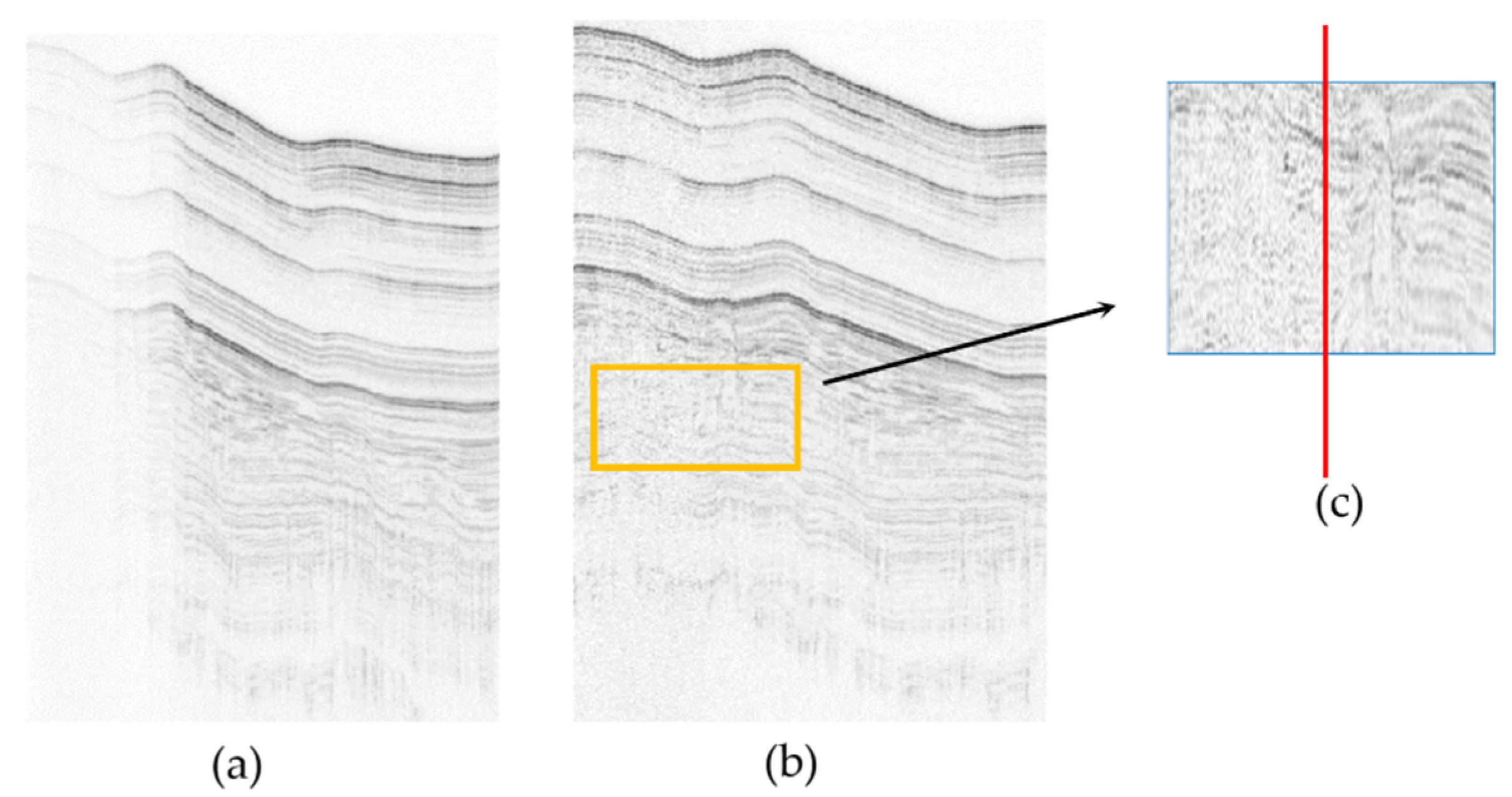
In this experiment, SBP data was recorded using a profiler named ATLAS PARASOUND 70 (Made by Teledyne Marine). This profiler can transmit an frequency modulation (FM) pulse that is linearly swept from 2 to 8 kHz, with a time duration of 50 ms. The water depth in the measured area varies from 1000 to 1200 m. To carry out this measurement, a deep-towed system has been used. The distance between the seabed and the deep-towed system was about 80 m. Because of the instability of the surveying system, some pings may have relatively low intensities. As shown in Figure 7a, the left part of Figure 7a has a low level of intensity, and the sediment details will not be recognized well. Referencing this intensity difference, the range of the polluted pings can be determined. In this measurement, the polluted pings start from 1st ping and end at the 130th ping. Referencing the 131st ping, the histogram matching method was applied to the 1st~130th pings, and the intensities of these pings have been adjusted. Though the intensities have been adjusted, the data is seriously influenced by noise, as shown in Figure 7c. Because the noise level is close to the intensity of sediment reflection, the reflection signals will not be separated from noise well.

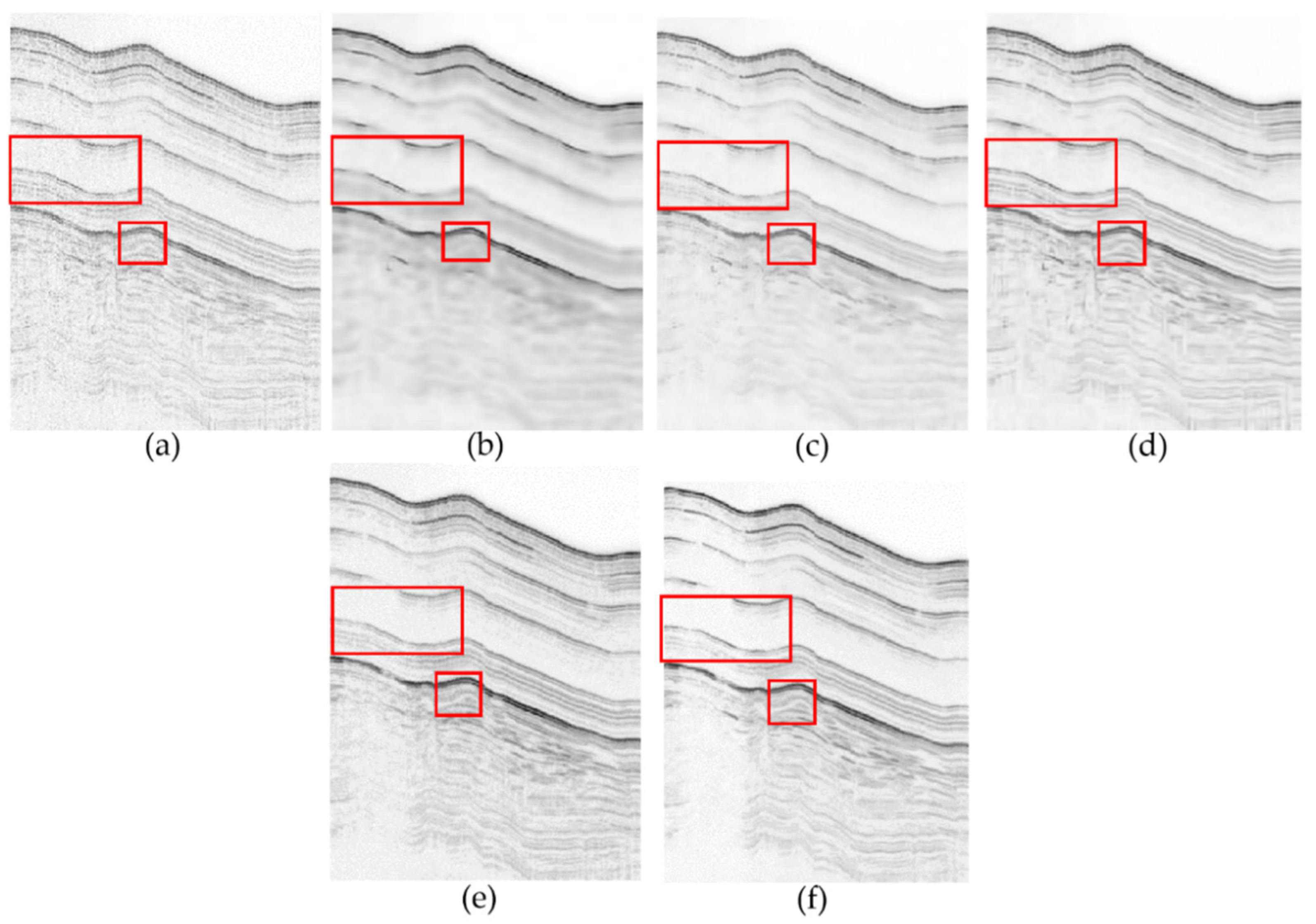
To improve the quality of this SBP image, the proposed method was applied. Firstly, a guidance image was obtained according to Section 2.2. As shown in Figure 8b, different colors represent different direction information. With the direction information constraint, guidance weight was calculated and was combined with the non-local low-rank framework to denoise the SBP image. The final filtered image is shown in Figure 9f. Thanks to the guidance weight constraint, our results removed noise well.

We also compared the proposed method for SBP image denoising, to the following widely used filtering methods: KSVD [26], NLM [7], BM3D [8], and the conventional non-local low-rank filtering method without guidance weight constraint (combining the non-local method and the Split-SPCP low-rank optimization method, referred to as NLLR in this paper).

The result using KSVD filtering is shown in Figure 9b. The layering structures are destroyed in Figure 9b, which means a serious over-smoothing. Figure 9c shows the result using the NLM method. Some noise in the sediment interior has been removed. However, in the area where layering structures are distributed closely, details are seriously blurred. The performance of NLM denotes that obtaining clear patch groups is important and proves the superiority of the non-local low-rank framework filtering indirectly. Figure 9d shows the result processed by the BM3D denoising method and the over-smoothing phenomenon still exists in Figure 10d. The conventional non-local low-rank method, NLLR, has removed most of the noise, and layering structures have been preserved. However, there still exists residual noise, as shown in Figure 10e,k, because of the incorrect similar patches’ selection. Compared with other methods, the proposed method achieved the best performance, as shown in Figure 9f and Figure 10f,l.

Another test dataset was downloaded from the open dataset [27]. The data was surveyed in the Gulf of Mexico with the sub-bottom profiler named EdgeTech 2200 M. The survey area has a water depth of about 1000 m. To carry out this measurement, an Autonomous Underwater Vehicle (AUV) has been used. The data quality is good, and the layering structures are displayed well. However, the scattering echoes in the sediment interior may bring difficulties to the following auto-processing, such as horizon picking and sediment classification. Different methods were applied to this denoising task and comparisons were made. KSVD and BM3D, as well as NLM preserved the layering structures well, however, the noise has not been removed well. BM3D generated some fake structures which were introduced into the filtered results, as shown in the area marked with red rectangles in Figure 11d. The NLLR method removed most of the noise, though there is still residual noise, as shown in the area marked with a red rectangle in Figure 11e. Thanks to the guidance weight constraint and the vertical constraint, our results removed noise well, as shown in Figure 11f. What is more, applying vessel enhancement filtering to the complementary image IM´ improved the performance of our method in sediment interior noise reduction.

3.3. Shallow-Sea Data Processing and Analysis

Data surveyed in shallow water using the C-Boom sub-bottom profiler were also adopted in the experiments. The used profiler system has a central frequency of 1.76 kHz, with the sampling interval of 0.1 ms. The water depth in the surveyed area varies from 5 to 15 m. During this measurement, because of the bad sea conditions, the SNRs of SBP images were low. As shown in Figure 12a, though sediment interfaces have been preserved in SBP images, the sediment interiors are filled with noise. The noise is thin stripe-like noise. In fact, during measurement, the sub-bottom profile received echoes continuously in the vertical direction ping by ping. Thus, noise in different pings is independent, but will influence the data quality continuously in the same ping.

The result using KSVD filtering is shown in Figure 12b. The performance of KSVD in this application scenario is not bad. The layering structures have been preserved well. However, there still remains residual noise. The result using NLM is shown in Figure 12c. The performance of NLM is the same as that of KSVD. In this situation, BM3D obtained a poor performance. Though layering structures are preserved, a lot of stripe-like noise is kept in the filtered image. What is more, the over-smoothing phenomena still exists in Figure 12d. Some vertical fake structures have been kept in the filtered result. as shown in Figure 12j. NLLR has removed most of the noise and reserved layering structures. However, because of the low accuracy in selecting similar patches, there still exists residual noise, as shown in Figure 12e. Thanks to the guidance weight constraint and the vertical constraint, our results removed noise well, as shown in Figure 12f. Another survey line surveyed in the same area was also used to verify the performance of our method, and the results are shown in Figure 13. The proposed method still has better performance than other methods.

3.4. Synthetic Data Processing and Analysis

For numerical comparisons, we applied different methods to the denoising of synthetic data. The PSNR and the SSIM were used to evaluate the performance. The equations used to compute both PSNR and SSIM are given by Alain Horé and Djemel Ziou [28]. The clean SBP image is generated by Gaussian function, since Gaussian function is usually used as an envelope function to amplitude modulation to an emitted wave [29]. Because the distribution of noise on SBP images is unknown, there is no rigorous way to simulate an SBP image containing noise. We treated the received signals in some special areas as noise. For example, there is no sediment interface reflection in the area of water column and sediment interior. The gray level changes in these areas are caused by environmental noise and other noise. Thus, we treated signals on SBP image in these areas as noise and intercepted them directly from the SBP image. After that, a simulated noise SBP image can be obtained by superimposing the intercepted information onto the clean SBP image.

As shown in Figure 14b,i, two different types of SBP images polluted by different noises are generated. Figure 14a,h show the clean images, and Figure 14c–g,j–n show the filtered images using different methods. The parameter settings of NLLR and the proposed method are as described in Section 3.1. The SSIM and PSNR of different filtered images are shown in

Table 1. Comparison of the different denoising methods applied in Figure 14b. Bold highlights indicate the best results.

	KSVD	NLM	BM3D	NLLR	Authors’ Method
SSIM	0.218	0.392	0.394	0.902	0.903
PNSR	15.871	16.347	16.296	23.091	23.097
Runtime	37.9 s	15.9 s	4.1 s	171.5 s	78.1 s

and

Table 2. Comparison of the different denoising methods applied in Figure 14i. Bold highlights indicate the best results.

	KSVD	NLM	BM3D	NLLR	Authors’ Method
SSIM	0.190	0.197	0.196	0.225	0.324
PNSR	10.049	11.09	10.937	20.897	21.9
Runtime	168.5 s	41.8 s	12.2 s	265.2 s	170.6 s

. The denoising performances of different methods have been qualitatively compared. It shows that the KSVD is not suitable for SBP image denoising. The performances of BM3D and NLM are better than KSVD. However, all of these methods described above achieved SSIM values lower than 0.4 and PSNR values lower than 17. The performance of the NLLR method is far better than the methods described above, which means that the non-local framework is suitable for SBP image denoising. The proposed method achieved the best results compared with other methods, an average SSIM of 0.614 and PSNR of 22.5, which proves that our method is especially suitable for SBP image denoising. The experiments were implemented on a computer with 16 GB RAM and an Intel Core i7-10750H @ 2.60 GHz. The runtime of different methods is also listed in Table 1 and Table 2. The proposed method and NLLR spent more runtime than other methods. However, because of the improved accuracy in selecting similar patches, the proposed method takes less time to solve Equation (16) than NLLR and the total runtime of the proposed method is also less than NLLR.

Similarly, the filtering results and runtime in Figure 15 can be obtained and are shown in

Table 3. Comparison of the different denoising methods applied in Figure 15b. Bold highlights indicate the best results.

	KSVD	NLM	BM3D	NLLR	Authors’ Method
SSIM	0.391	0.394	0.397	0.898	0.906
PNSR	16.151	16.841	16.287	22.077	22.330
Runtime	41.2 s	16.7 s	4.5 s	192.3 s	87.2 s

and

Table 4. Comparison of the different denoising methods applied in Figure 15i. Bold highlights indicate the best results.

	KSVD	NLM	BM3D	NLLR	Authors’ Method
SSIM	0.181	0.185	0.182	0.214	0.216
PNSR	10.787	11.424	10.859	20.492	20.806
Runtime	158.8 s	42.9 s	12.4 s	267.1 s	172.7 s

(Figure 15 is obtained by changing the shapes of reflectors in Figure 14).

By changing the shapes of reflectors in Figure 14b, a set of synthetic data can be generated. Then, by applying filter methods to the data, and calculating the average value and standard deviation of each index (PSNR, SSIM, and Runtime), the statistical results can be obtained and are shown in

Table 5. The average (Av.) and standard deviation (SD) of indexes.

	KSVD	NLM	BM3D	NLLR	Authors’ Method
SSIM (Av. and SD)	0.355/ 0.077	0.398/ 0.013	0.395/ 0.001	0.899/ 0.002	0.903/ 0.003
PNSR (Av. and SD)	16.097/ 0.123	16.700/ 0.225	16.282/ 0.01	22.421/ 0.389	22.550/ 0.313
Runtime (Av. and SD)	39.2 s/ 1.65 s	15.9 s/ 0.61 s	3.72 s/ 0.78 s	181.3 s/ 9.53 s	83.4 s/ 3.74 s

. The proposed method achieved the average PSNR of 22.55 and SSIM of 0.903. Similarly, by changing the shapes of reflectors in Figure 14i, we can get the statistical results as shown in

Table 6. The average (Av.) and standard deviation (SD) of indexes.

	KSVD	NLM	BM3D	NLLR	Authors’ Method
SSIM (Av. and SD)	0.186/ 0.005	0.192/ 0.007	0.189/ 0.007	0.216/ 0.006	0.242/ 0.054
PNSR (Av. and SD)	10.411/ 0.418	11.247/ 0.183	10.891/ 0.54	20.525/ 0.256	20.990/ 0.612
Runtime (Av. and SD)	165.4 s/ 5.34 s	43.1 s/ 1.89 s	13.4 s/ 2.17 s	276.1 s/ 20.62 s	180.2 s/ 17.88 s

. The proposed method achieved the average PSNR of 20.99 and SSIM of 0.242.

In conclusion, the proposed method has better performance than other methods, as shown in Table 1, Table 2, Table 3, Table 4, Table 5 and Table 6, and NLLR obtained the second-best filtering performance.

4. Discussion

4.1. The Relationships between the Effects of Different Methods and SBP Image Characteristics

NLM, BM3D, NLLR, and the proposed method are based on the exploitation of SBP image non-local self-similarity, and these methods achieved better performances than KSVD, as shown in Table 1; Table 2. Since textures of different structures in different areas representing the same sediment interfaces are similar, the non-local self-similarity can be recognized as one of the inherent characteristics of a SBP image. Another characteristic of a SBP image is that the sediment interface extends in a particular direction and is displayed as a line-like structure on the SBP image. Then, the directions of these line-like structures can be used as auxiliary information for similar patches searching. Thus, based on the above two characteristics, the proposed method achieved excellent performance.

Compared with methods based on the non-local low-rank framework, performances of NLM and BM3D are poor in most cases. NLM does not consider the sparsity characteristics, while sparsity characteristics have been proven to be important for ultrasonic image denoising [12,17,19,25]. BM3D is very effective in Gaussian noise denoising [8]. However, sonar images are always polluted by scattered echoes [17], and scattered echoes on rough seabed surface can produce speckle noise. Moreover, the stripe noise also exists on the SBP image. Thus, the performance of BM3D is limited.

4.2. Limitations and Future Work of the Proposed Method

The proposed method has a large time cost. What is more, the proposed method can only process SBP images. However, the sub-bottom profiler can provide full-waveform data. Full-waveform data can be converted into instantaneous amplitude data and instantaneous phase data. The SBP image is formed based on instantaneous amplitude data, while instantaneous phase data has not been taken into consideration. To overcome these limitations, we will further extend the method to simultaneously filter instantaneous amplitude data and instantaneous phase data, which may help improve the fidelity of the filtered result. In future work, it is also important to realize real-time SBP image denoising.

5. Conclusions

The developed SBP image denoising method effectively overcomes the limitations of other methods and successfully obtained high-quality SBP images. Considering that the direction of layering structures is an important inherent characteristic in SBP images, the proposed filtering method firstly uses the vessel enhancement filtering to obtain the direction image and uses it as the guidance image, then calculates the guidance weight based on the guidance image. Guidance weight improves the accuracy of similar patches’ searching in the low-rank framework. Therefore, the method can efficiently filter out noise and maintain the real topography structures. Verified by the synthetic images’ denoising experiments, the proposed method achieved the total average PSNR of 21.77 and SSIM of 0.573, which is far better than other methods. However, the proposed method also has limitations. The proposed method can only denoise the SBP image, so we will further extend the method to simultaneously filter instantaneous amplitude data and instantaneous phase data. In future work, it is also important to realize real-time SBP image denoising. Note that the source code of the proposed method is available at: https://github.com/xingzhewujiangboboniao?tab=repositories.

References

1. Wilken, D.; Wunderlich, T.; Feldens, P.; Coolen, J.; Preston, J.; Mehler, N. Investigating the Norse Harbour of Igaliku (Southern Greenland) Using an Integrated System of Side-Scan Sonar and High-resolution Reflection Seismics. Remote Sens. 2019, 11, 1889. [Google Scholar] [CrossRef] [Green Version]
2. Gournia, C.; Fakiris, E.; Geraga, M.; Williams, D.P.; Papatheodorou, G. Automatic Detection of Trawl-Marks in Sidescan Sonar Images through Spatial Domain Filtering, Employing Haar-Like Features and Morphological Operations. Geosciences 2019, 9, 214. [Google Scholar] [CrossRef] [Green Version]
3. Fakiris, E.; Blondel, P.; Papatheodorou, G.; Christodoulou, D.; Dimas, X.; Georgiou, N.; Kordella, S.; Dimitriadis, C.; Rzhanov, Y.; Geraga, M.; et al. Multi-Frequency, Multi-Sonar Mapping of Shallow Habitats—Efficacy and Management Implications in the National Marine Park of Zakynthos, Greece. Remote Sens. 2019, 11, 461. [Google Scholar] [CrossRef] [Green Version]
4. Shang, X.; Zhao, J.; Zhang, H. Obtaining High-Resolution Seabed Topography and Surface Details by Co-Registration of Side-Scan Sonar and Multibeam Echo Sounder Images. Remote Sens. 2019, 11, 1496. [Google Scholar] [CrossRef] [Green Version]
5. Zhao, J.; Li, S.; Zhang, H.; Feng, J. Comprehensive Sediment Horizon Picking from Subbottom Profile Data. IEEE J. Ocean. Eng. 2019, 44, 524–534. [Google Scholar] [CrossRef]
6. Maroni, C.S.; Quinquis, A.; Vinson, S. Horizon Picking on Sub-bottom Profiles Using Multiresolution analysis. Digit. Signal Prog. 2001, 11, 269–287. [Google Scholar] [CrossRef]
7. Buades, A.; Coll, B.; Morel, J. Non-Local Means Denoising. Image Process. Line 2011, 1, 208–212. [Google Scholar] [CrossRef] [Green Version]
8. Dabov, K.; Foi, A.; Katkovnik, V.; Egiazarian, K. Image Denoising by Sparse 3-d Transform-domain Collaborative Filtering. IEEE Trans. Signal Process. 2007, 16, 2080–2095. [Google Scholar] [CrossRef] [PubMed]
9. Dong, W.; Li, X.; Zhang, L.; Shi, G. Sparsity-based Image Denoising via Dictionary Learning and Structural Clustering. In Proceedings of the Computer Vision and Pattern Recognition (CVPR2011), Colorado Springs, CO, USA, 20–25 June 2011; pp. 457–464. [Google Scholar] [CrossRef]
10. Zuo, W.; Zhang, L.; Song, C.; Zhang, D. Texture Enhanced Image Denoising via Gradient Histogram Preservation. In Proceedings of the Computer Vision and Pattern Recognition (CVPR2013), Portland, OR, USA, 23–28 June 2013; pp. 1203–1210. [Google Scholar] [CrossRef] [Green Version]
11. Zhou, X.; Yang, C.; Zhao, X.; Yu, W. Low-rank Modeling and its Applications in Image Analysis. ACM Comput. Surv. 2014, 47, 1–33. [Google Scholar] [CrossRef] [Green Version]
12. Zhu, L.; Fu, C.; Brown, M.S.; Heng, P. A Non-local Low-rank Framework for Ultrasound Speckle Reduction. In Proceedings of the Computer Vision and Pattern Recognition (CVPR2017), Hawaii, HI, USA, 25–30 June 2017; pp. 493–501. [Google Scholar] [CrossRef]
13. Xie, N.; Chen, Y.; Liu, H. 3D Tensor Based Nonlocal Low Rank Approximation in Dynamic PET Reconstruction. Sensors 2019, 19, 5299. [Google Scholar] [CrossRef] [PubMed] [Green Version]
14. Shang, Z.; Zhao, C.; Wan, J. Application of Multi-resolution Analysis in Sonar Image Denoising. J. Syst. Eng. Electron. 2008, 19, 1082–1089. [Google Scholar] [CrossRef]
15. Firoiu, I.; Nafornita, C.; Isar, D.; Isar, A. Bayesian Hyperanalytic Denoising of Sonar Images. IEEE Geosci. Remote Sens. Lett. 2001, 8, 1065–1069. [Google Scholar] [CrossRef]
16. Wang, X.; Liu, A.; Zhang, Y.; Xue, F. Underwater Acoustic Target Recognition: A Combination of Multi-Dimensional Fusion Features and Modified Deep Neural Network. Remote Sens. 2019, 11, 1888. [Google Scholar] [CrossRef] [Green Version]
17. Jin, Y.; Ku, B.; Ahn, J.; Kim, S.; Ko, H. Nonhomogeneous Noise Removal from Side-scan Sonar Images Using Structural Sparsity. IEEE Geosci. Remote Sens. Lett. 2019, 16, 1–5. [Google Scholar] [CrossRef]
18. Lurton, X. An Introduction to Underwater Acoustic: Principles and Applications, 2nd ed.; Springer: Chichester, UK, 2010; pp. 372–379. [Google Scholar]
19. Manj´on, J.V.; Coup´e, P.; Buades, A. MRI Noise Estimation and Denoising Using Non-local PCA. Med. Image Anal. 2015, 22, 35–47. [Google Scholar] [CrossRef] [PubMed]
20. Frangi, A.F.; Niessen, W.J.; Vincken, K.L.; Viergever, M.A. Multiscale Vessel Enhancement Filtering. In Proceedings of the International Conference on Medical Image Computing and Computer-Assisted Intervention (MICCAI1998), Cambridge, MA, USA, 11–13 October 1998; pp. 130–137. [Google Scholar] [CrossRef] [Green Version]
21. Sun, Q.; Xiang, S.; Ye, J. Robust Principal Component Analysis via Capped Norms. In Proceedings of the 19th ACM International Conference on Knowledge Discovery and Data Mining(SIGKDD2013), Chicago, IL, USA, 11–14 August 2013; pp. 311–319. [Google Scholar] [CrossRef]
22. Gu, S.; Zhang, L.; Zuo, W.; Feng, X. Weighted Nuclear Norm Minimization with Application to Image Denoising. In Proceedings of the IEEE Conference on Computer Vision and Pattern Recognition (CVPR2014), Columbus, OH, USA, 24–27 June 2014; pp. 2862–2869. [Google Scholar] [CrossRef] [Green Version]
23. Lu, C.; Zhu, C.; Xu, C.; Yan, S.; Lin, Z. Generalized Singular Value Thresholding. arXiv 2014, arXiv:1412.2231. [Google Scholar]
24. Driggs, D.; Becker, S.; Aravkin, A. Adapting Regularized Low-rank Models for Parallel Architectures. SIAM J. Sci. Comput. 2019, 41, 163–189. [Google Scholar] [CrossRef] [Green Version]
25. Coupé, P.; Hellier, P.; Kervrann, C.; Barillot, C. Nonlocal Means-based Speckle Filtering for Ultrasound Images. IEEE Trans. Image Process. 2009, 18, 2221–2229. [Google Scholar] [CrossRef] [PubMed] [Green Version]
26. Aharon, M.; Elad, M.; Bruckstein, A.M. K-SVD: An Algorithm for Designing Overcomplete Dictionaries for Sparse Representation. IEEE Trans. Signal Process. 2006, 54, 4311–4322. [Google Scholar] [CrossRef]
27. Fisher, C. Acute Response of Benthic Hard Bottom Communities to Oil Exposure in the Deep Gulf of Mexico. Available online: http://www.marine-geo.org/tools/search/entry.php?id=AT18-03 (accessed on 1 May 2020).
28. Hore, A.; Ziou, D. Image quality metrics: PSNR vs. SSIM. In Proceedings of the 2010 20th International Conference on Pattern Recognition (ICPR), Istanbul, Turkey, 23–26 August 2010; pp. 2366–2369. [Google Scholar] [CrossRef]
29. Mohamed, S. Sediment Classification Using Sub-bottom Profiler. Master’s Thesis, Delft University of Technology, Delft, The Netherlands, 2011. [Google Scholar]
Figure 1. Illustration of patch searching and patch group construction. The different colored rectangles in (a) represent patches with different similarities, (b) denotes a patch group, and (c) is the constructed low-rank matrix.
Remotesensing 12 02336 g001
Figure 2. An overview of the proposed filtering framework. (a) is the original SBP image. First, the guidance image (b) is computed based on (a) to help the selection of similar patches. Then, after patch grouping (rectangles in (c) represent patches) and low-rank optimization ((d) is the optimization diagram), the patches are refined, and the low-rank structures are recovered as shown in (e). Aggregating all of the low-rank patches, the final result (f) is obtained.
Remotesensing 12 02336 g002
Figure 3. Illustration of sub-bottom profile (SBP) measurement, (a) shows that the measurement of the sub-bottom profile can capture the information of sediment, (b) shows the received reflection echoes, and (c) is the final cross-section image of the sub-bottom. The red rectangles in (c) represent the sediment interior and the green rectangle represents the sediment interface.
Remotesensing 12 02336 g003
Figure 4. Illustration of the guidance weight, (a) shows the locations of the reference patch and the searching patches, (b) illustrates the relative direction between the reference patch and the searching patch, (c) and (d) visualize the functions Ψ´(η´) and Ψ(η), respectively.
Remotesensing 12 02336 g004
Figure 5. Illustration of parameter settings. (a) and (b) show the first synthetic clean SBP image and the polluted SBP image, respectively. (c) shows the peak signal-to-noise ratio (PSNR) surface and the red point has the highest value, (d) shows the structural similarity index (SSIM) surface obtained similarly to the PSNR surface and the red point has the highest value.
Remotesensing 12 02336 g005
Figure 6. Illustration of parameter settings. (a) and (b) show the second synthetic clean SBP image and the polluted SBP image, respectively, (c) shows the PSNR surface and the red point in (c) has the highest PSNR value, (d) shows the SSIM surface obtained similarly to the PSNR surface. The red point in (d) is a local maximum point and the black point in (d) has the highest SSIM value.
Remotesensing 12 02336 g006
Figure 7. The original SBP image and the SBP image after histogram matching, (a) is the original SBP image, (b) is the SBP image after grayscale equalization, (c) shows details in the area marked with a yellow rectangle in (b). (c) shows that the rectangle area in (b) is separated into two parts having different Signal-to-Noise Ratio (SNR) and the left part has a low SNR.
Remotesensing 12 02336 g007
Figure 8. The SBP image after histogram matching and its corresponding direction information, (a) is the SBP image after grayscale equalization, and (b) shows the direction information.
Remotesensing 12 02336 g008
Figure 9. Filtering results: (a) is the SBP image after grayscale equalization, (bf) are the filtered results using KSVD, Non-local Means (NLM), Block-Matching and three-dimensional (3D) filtering (BM3D), the conventional non-local low-rank filtering method (NLLR), and the proposed method.
Remotesensing 12 02336 g009
Figure 10. Filtering results: (a) is the details of the area in the lower rectangle in Figure 9a, (bf) show the details of filtered results in the lower rectangle in Figure 9 using KSVD, NLM, BM3D, NLLR, and the proposed method, (g) is the details of the area in the top rectangle in Figure 9a, (hl) are the details of filtered results in the top rectangle using KSVD, NLM, BM3D, NLLR, and the proposed method.
Remotesensing 12 02336 g010
Figure 11. Filtering results: (a) is the SBP image, (bf) are the filtered results using KSVD, NLM, BM3D, NLLR, and the proposed method, (g) shows the details of the SBP image in the rectangle area in Figure 11a, (hl) are filtered results in the rectangle area in Figure 11a using KSVD, NLM, BM3D, NLLR, and the proposed method.
Remotesensing 12 02336 g011
Figure 12. Filtering results: (a) is the SBP image, (bf) are the filtered results using KSVD, NLM, BM3D, NLLR, and the proposed method, (g) shows the details of the SBP image in the rectangle area in Figure 12a, (hl) are the filtered results in the rectangle area in Figure 12a using KSVD, NLM, BM3D, NLLR, and the proposed method.
Remotesensing 12 02336 g012
Figure 13. Filtering results: (a) is the SBP image, (bf) are the filtered results using KSVD, NLM, BM3D, NLLR, and the proposed method, (g) is the details of the SBP image in the rectangle area in Figure 13a, (hl) are the filtered results in the rectangle area in Figure 13a using KSVD, NLM, BM3D, NLLR, and the proposed method.
Remotesensing 12 02336 g013
Figure 14. Filtering results based on synthetic data: (a) shows the clean synthetic SBP image, (b) is the synthetic polluted SBP image, (cg) are the filtered results using KSVD, NLM, BM3D, NLLR, and the proposed method, (h) is the clean synthetic SBP image, (i) is a synthetic polluted SBP image, (jn) show the filtered results using KSVD, NLM, BM3D, NLLR, and the proposed method.
Remotesensing 12 02336 g014
Figure 15. Filtering results based on synthetic data: (a) shows the clean synthetic SBP image, (b) is the synthetic polluted SBP image, (cg) are the filtered results using KSVD, NLM, BM3D, NLLR, and the proposed method, (h) is the clean synthetic SBP image, (i) is a synthetic polluted SBP image, (jn) show the filtered results using KSVD, NLM, BM3D, NLLR, and the proposed method.
Remotesensing 12 02336 g015