A New GNSS-Derived Water Vapor Tomography Method Based on Optimized Voxel for Large GNSS Network

Abstract

The Global Navigation Satellite System (GNSS) tomographic technique can be used for remote sensing of the three-dimensional water vapor (WV) distribution in the troposphere, which has attracted considerable interest. However, a significant problem in this technique is the excessive reliance on constraints (particularly in large GNSS networks). In this paper, we propose an improved tomographic method based on optimized voxel, which only considers the voxels passed by GNSS rays. The proposed method can completely prevent the tomographic algorithm interference of constraints that originated from empirical functions. Experiments in Nanjing in the periods of day-of-year (DOY) 182–184, 2019, and 244–246, 2019, show that the mean absolute error (MAE) and root mean square error (RMSE) of the WV density profile obtained using the proposed method are 0.9 and 1.3 g/m³, while those obtained using the conventional method are 1.3 and 1.8 g/m³, respectively, with respect to the radiosonde (RS) method. The numerical results show that the proposed method is reliable and has a superior accuracy to that of the conventional method.

1. Introduction

Considering the advantages of increasing global navigation satellite system (GNSS) constellations and the extensive construction of continuous operation reference stations (CORSs), GNSS-derived water vapor (WV) information has gradually become a vital resource of tropospheric WV production [1,2,3]. With its all-time all-weather support and high spatial-temporal resolution, the GNSS remote WV detection technique can be used to track the dynamic variation in tropospheric WV based on real-time or near-real-time data transmission of the CORS system [4,5,6]. This provides sufficient data for numerical weather forecasting and disaster weather warning [1,7,8,9].

The application of the GNSS in water vapor detection was initially proposed by Bevis et al. [1] in 1992. The original WV product is two-dimensional (2D) precipitable WV (PWV) retrieved from GNSS observations, having the same accuracy as those of the measures obtained using the traditional meteorological technology (e.g., radiosonde (RS) and WV radiometer), which has attracted considerable attention [10,11,12]. Furthermore, extensive GNSS WV remote sensing experiments have been carried out worldwide, including those in China [13], North America [14], and Europe [15], which jointly verify the reliability of the GNSS-derived PWV.

In recent years, a novel promising approach is to reconstruct the three-dimensional (3D) WV distribution by GNSS observations [6,16,17,18,19,20,21,22,23,24,25,26,27]. This technique for 3D WV product acquisition based on the GNSS system is referred to as GNSS WV tomography. Although this WV tomographic method has been developed by Flores et al. [18] in 2000, numerous challenges still exist. The main drawbacks in GNSS WV tomography, particularly in a large GNSS network (such as the Nanjing area), are ill-posed problems caused by null-ray voxels or sparse station [18,24,27,28], and complex computation for the inverse of the coefficient matrix as it is large and sparse [19,21].

Numerous studies have been carried out to overcome these problems, which have led to remarkable results. For example, Flores et al. [18] imposed constraints on tomographic equations that significantly increased the rank score of the tomographic coefficient matrix. This measure is beneficial for the tomographic equation solution and thus, was widely used by other scientists [17,23,25,26,27]. Zhao et al. [25] maximized the usage of GNSS observations by including the signals leaving the side face of the tomographic zone in the tomographic process by a global pressure and temperature 2 wet (GPT2w) model, in addition to the general effective signals (i.e., signals penetrating the top layer of the tomographic zone to the receivers). Similarly, Zhang et al [29] used the side signal by a novel height factor model (HFM). Zhao et al. [26] and Dong et al. [17] improved the utilization of effective signals by combining multi-GNSS observations (global positioning system (GPS), Beidou, global navigation satellite system (GLONASS), and Galileo). Furthermore, they verified the approach in, respectively, Guiyang and Hong Kong, China. In the aspect of ill-posed tomography model resolving, Zhao et al. [30] adopted an improved ridge estimation (IRE) method to revise the singular in the tomographic coefficient matrix, and numerical results indicate its superior performance compared to the commonly used singular value decomposition (SVD) method. Notably, the above WV tomographic experiments rely on constrains, and massive constraints tend to decrease the role of GNSS observations in the tomographic results [24].

To completely avoid the dependence on these constraints generated from empirical functions, in this study, an optimized tomographic algorithm with voxel redistribution is proposed, based on the principle of elimination of all the null-ray-passed voxels. We establish a new constraint that originates from GNSS-derived PWV that fits the actual distribution of WV (Section 2). The optimized tomographic method is validated in the Nanjing area (Section 3). A conclusion is presented in Section 4.

2. Data and Methods

2.1. 2D WV Productions by GNSS Observations

The 2D WV productions, called PWV, can be retrieved from GNSS observations. A commonly used tropospheric delay in the PWV processing is the tropospheric zenith total delay (ZTD), which is estimated by the observations, subtracted from the zenith hydrostatic delay (ZHD), and calculated by an empirical model (e.g., the Saastamoinen model [31]), and which yields the zenith wet delay (ZWD). The PWV of each site can be retrieved from the ZWD through the conversion coefficient. Additionally, in a relatively dense CORS network, the PWVs derived from multi-stations can provide a 2D WV field in the station coverage area by interpolation [13].

$$\mathrm{ZWD}=\mathrm{ZTD}-\mathrm{ZHD},$$

(1)

$$\mathrm{PWV}=\prod \times \mathrm{ZWD},$$

(2)

where $\prod$ is the conversion parameter used to convert $\mathrm{ZWD}$ to $\mathrm{PWV}$, and

$$\prod =\frac{{10}^6}{{\rho }_w\times R_v\times (\frac{k_3}{T_m}+k^{\prime }{}_2)},$$

(3)

where ${\rho }_w$ and $R_v$ are the density of liquid water and universal gas constant, respectively; $k_3$ and $k^{\prime }{}_2$ are empirical constants [32]; and $T_m$ is the weighted mean temperature, a function of surface meteorological factors (e.g., surface temperature, pressure, and relative humidity). In this study, we used the Bevis model [1] to obtain $T_m$.

2.2. 3D WV Productions by GNSS Observations

The 2D PWV product has limited applications in meteorology. Flores et al. [18] have proposed the 3D WV product through a tomographic algorithm in Hawaii based on GNSS observations. In the algorithm, the slant wet delay (SWD) is the key parameter, and is obtained by restoring the ZWD to the GNSS ray propagation direction. We use the following equation to calculate the SWD of each signal,

$$\mathrm{SWD}=\mathrm{ZWD}·M_w\left(E\right)+M_{\Delta }\left(E\right)·\left(G_{NS}\cos A+G_{WE}\sin A\right)+R,$$

(4)

where $E$ and $A$ are the elevation angle and azimuth angle of the satellite; $M_w\left(E\right)$ and $M_{\Delta }\left(E\right)$ are the wet mapping function and gradient mapping function; $G_{NS}$ $G_{WE}$ are the horizontal gradients in the north–south and east–west directions, respectively; and $R$ is a residual term. We can then obtain the slant WV (SWV) by

$${\mathrm{SWV}}_i^m=\prod \times {\mathrm{SWD}}_i^m,$$

(5)

where $m$ and $i$ are the GNSS station serial number and satellite serial number, respectively. $\prod$ is obtained by Equation (3).

After the retrieval of the SWV of each signal, the objects covered by the GNSS stations need to be divided into a finite number of voxels. Owing to these voxels, an integral signal is discretized into several line segments. Therefore, the complete SWV carried by a ray is divided into several parts by voxels; each part represents the moisture content of its voxel. Through a large number of such rays, the 3D moisture field in the objects can be reconstructed. The above process can be described by

$${\mathrm{SWV}}^m={\displaystyle \sum {}_{ijk}\left(A_{ijk}^m·X_{ijk}\right)},$$

(6)

where ${\mathrm{SWV}}^m$ is the SWV of the effective signal $m$ passing through the top boundary of the objective area. Only such signals can be used for the next processing, because the SWVs carried by them are completely included in the study area. Notably, differing from Equation (5), the $m$ refers to the serial number of an effective signal whose quantity was determined by both GNSS stations and satellites. $A_{ijk}^m$ is the intercept of the signal $m$ in voxel $\left(i,j,k\right)$. $X_{ijk}$ is the corresponding WV density of the voxel. Based on the effective signal with the SWV at an epoch, we obtain the observation equation,

$$Ax=d,$$

(7)

where $A$ is the coefficient matrix composed of the signal intercept, $d$ is the column vector of all the effective SWV observations, and $x$ is a column vector of unknown parameters that represent the WV density in each voxel. Overall, the 3D WV product can be obtained by solving the linear Equation (7) according to the GNSS observations.

2.3. Conventional Solution for WV Tomography

As shown in Figure 1, owing to the unsatisfactory geometric distribution of satellite constellations and ground receivers, inevitably, some voxels are not passed by any signal. This demonstrates that Equation (7), is ill-posed. Moreover, the problem becomes more significant for sparser receivers [24]. Thus, some constraints are required to stabilize Equation (7). The WV density in a certain voxel can be determined by its surrounding voxels [18,33]. Based on the above theory, the general method for WV tomographic equation solution introduces the following three types of constraints.

(1) Horizontal Constraint

These constraints are used to determine the WV value in null-ray passed voxels according to their neighbors in the same level [18], which can be described:

$$H\times X=0,$$

(8)

where $H$ is the constraint matrix for the horizontal direction.

(2) Vertical Constraint

The relation between the WV densities of two vertically adjacent voxels can be expressed by the vertical constraint expressed as:

$$V\times X=0,$$

(9)

where $V$ stands for vertical constraint matrix.

(3) Boundary Constraint

The tropospheric WV density rapidly decreases with the increase in height. In this case, we assume that the WV density in the top-layer voxels is zero. Accordingly, in addition to the horizontal and vertical constraints, we add the following top-level boundary constraints,

$$B\times X=0.$$

(10)

Considering the above three types of constraint equations, the coefficient matrix $A$ and result matrix $d$ in Equation (7) (i.e., original tomographic equation) are modified to

$$A_{new}=\left[\begin{array}{c}{A}_{ori}\\ H\\ V\\ B\end{array}\right], d=\left[\begin{array}{c}{d}_{ori}\\ 0\\ 0\\ 0\end{array}\right].$$

(11)

However, even with the expanded coefficient matrix $A$ and $d$ (Equation (11)), an ill-posed problem exists in Equation (7) owing to the limited effective observations in one epoch. To overcome this problem, we multiply the rows of matrix $A_{ori}$, which is composed of original GNSS observations, by setting a “tomography window.” The tomographic window is based on the assumption that the WV content is stationary in a period of time and can significantly expand matrix $A_{ori}$ through multi-epoch observations.

After the above process steps, the solution of the updated Equation (7), i.e., the value of $x$, expresses the WV density in each voxel of the tomographic region. However, considering that the coefficient matrix composed of observations and constraints is a large-scale sparse matrix with the corresponding inverse problem, it is challenging to obtain $x$. Two main methods can be used to solve the tomographic equations, including non-iterative and iterative algorithms [17]. The latter exhibits a higher performance than that of the former. Among the iterative methods, the multiplicative algebraic reconstruction technique algorithm [17] and Kalman filtering (KF) technique [34,35] have been widely used. The KF technique includes an advanced algorithm, simple implementation, and good performances in numerous fields. Thus, we use KF to solve the tomographic equations. Besides, references [36,37] describe the KF for tomographic use in detail.

Overall, the general tomographic approach introduces auxiliary constraints (horizontal, vertical, and boundary constraints) into the original tomographic Equation (7) to solve its ill-posed problem and obtain its solutions through an iterative algorithm (such as the KF in this case).

2.4. Optimized Solution for WV Tomography

Regarding the conventional tomographic approach, the additional constraints are some virtual observations generated from the empirical function, which may lead to solutions against the truth. Therefore, the optimal WV tomography approach should reduce the dependence on constraints as much as possible.

Another problem is the underlying causes of the rank deficiency of matrix $A$. Besides the null-signal-passed voxels, massive linear dependence equations exist in Equation (7), which also leads to the rank deficiency of matrix $A$.

The origin of the existence of the too large number of linear dependence equations is visualized in Figure 2. We assume that the satellite elevation cut-off is 10° (minimum elevation cut-off angle allowed in GNSS data processing). A signal emerges from the satellite, intersects with the 8-km-high tropopause at point (c), and finally reaches the receiver (a). The segment (a–b) is the projection of the signal line segment (a–c) on the ground with a length of approximately 45 km. This is the maximum span of a signal segment, in theory. In practice, only a few signals have elevation angles close to 10°, which indicates that most signal ground projections (such as (a–b) in Figure 2) are considerably shorter than 45 km. Hence, in the tomographic region, far station spacing or sparse grids can lead to a significant number of signals only passing through voxels in the same column. The tomographic equations consisting of these rays can exhibit obvious linear dependence. In other words, after the elementary row transformation, only a few nonzero lines of the coefficient matrix $A$ in Equation (7) remain.

To solve the second problem, a smaller grid spacing can be designed that will significantly increase the number of voxels. More voxels imply more null-ray-passed voxels, which leads to a worse ill-posed problem in the tomographic equation. Hence, we need to impose more constraints to overcome the above problem. However, these constraints may bias the tomographic results. Thus, we may not simultaneously overcome the two shortcomings in the conventional tomographic approach via a single approach; if the second problem is solved, the first problem would be more complex, and vice versa.

In this study, we propose a novel tomographic approach, based on the principle of the elimination of null-ray-passed voxels. It can simultaneously reduce the contradictory disadvantages encountered in the traditional approach. We present the optimized tomographic approach in Figure 3.

Figure 3a shows a 3D cube divided into a $3\times 3\times 3$ grid, which represents a tomographic area composed of 27 self-enclosed 3D voxels. Figure 3b shows the tomographic zone and several visualized rays from three sites. This simulates the penetration of the voxel by rays. Most voxels are penetrated by rays, but a few voxels, particularly those at the bottom, are not penetrated. In this regard, the traditional tomographic method imposes constraints on the first layer in the tomographic zone, which act as virtual signals, so that almost all voxels are passed-through by signals. This increases the rank score of the tomographic coefficient matrix but introduces errors to the results. Hence, we propose a new WV tomographic technique, i.e., voxel redistribution, which does not depend on constraints originating from empirical functions. As shown in Figure 3c, the modified tomographic zone eliminates all voxels without signal penetration, which, to some extent, reduces the number of estimates, but significantly mitigates the rank deficiency problem of the tomographic coefficient matrix. Additionally, based on the above principle, we use Equations (12)–(15) to auxiliarily describe the voxel redistribution.

$$X_{ori}={\left[x_1,x_2,x_3,x_4,x_5,x_6,x_7,x_8,x_9, \dots x_{13}, \dots x_{27}\right]}^T,$$

(12)

$$X_{temp}={\left[\bcancel{x_1},x_2,\bcancel{x_3},\bcancel{x_4},x_5,x_6,\bcancel{x_7},x_8,\bcancel{x_9}, \dots \bcancel{x_{13}}, \dots x_{27}\right]}^T,$$

(13)

$$X_{upd}={\left[x_1,x_2,x_3, \dots x_{21}\right]}^T,$$

(14)

$$X_{final}={\left[\mathrm{null},x_1,\mathrm{null},\mathrm{null},x_2,x_3,\mathrm{null},x_4,\mathrm{null}, \dots ,x_7,\mathrm{null},x_9 \dots x_{21}\right]}^T,$$

(15)

where $X_{ori},X_{temp},X_{upd}$, and $X_{final}$ represent the original voxels (i.e., all voxels in the tomographic area), temporary voxels (only the null-ray-passed part is removed, but without renumbering), updated voxels (renumbered based on the temporary voxels), and final voxels (processed to restore the upgraded voxel according to its geometric location), respectively. $X_{upd}$ is the estimate matrix (i.e., WV density matrix) in the tomographic equation, which can be reconstructed to a form similar to that of $X_{final}$ after its values are obtained.

In summary, the voxels in the tomographic zone with sequential numbers are screened to pass by at least one ray. The WV density of these voxels is then computed by the tomographic equation. Finally, the voxels with WV information are re-sorted according to their original numbers, while the null-ray-passed voxels are assigned a “null” value. Regarding these “null” values, we can estimate their WV density by interpolation. Based on the above technique, we can reasonably reconstruct the 3D WV distribution in the object zone.

Furthermore, we introduce a new PWV constraint, established by the GNSS-derived PWV, which differs from the above general constraints. This constraint is consistent with the actual tropospheric WV distribution,

$$P\times X=PWV$$

(16)

where $P$ is the coefficient matrix of the PWV constrains, while $PWV$ is the corresponding result matrix. As shown in Figure 4, we can establish a unique vertical constraint (PWV constraint) in the column grid where a GNSS station is located. We assume a signal penetrating the tomographic region from the zenith and finally reaching the receiver. This virtual signal line is discretized into several segments by the voxels. Nevertheless, we set one for every segment following the physical distribution of PWV. These segments form the constraint coefficient matrix $P$. The PWV value corresponding to the ray forms the result matrix $PWV$.

3. Experiment and Validation

To assess the optimized tomographic algorithm, we design a comparative experiment between the conventional and proposed approaches. First, we describe the study area (Nanjing) and data processing. The experimental results and comparison between the two approaches are then presented.

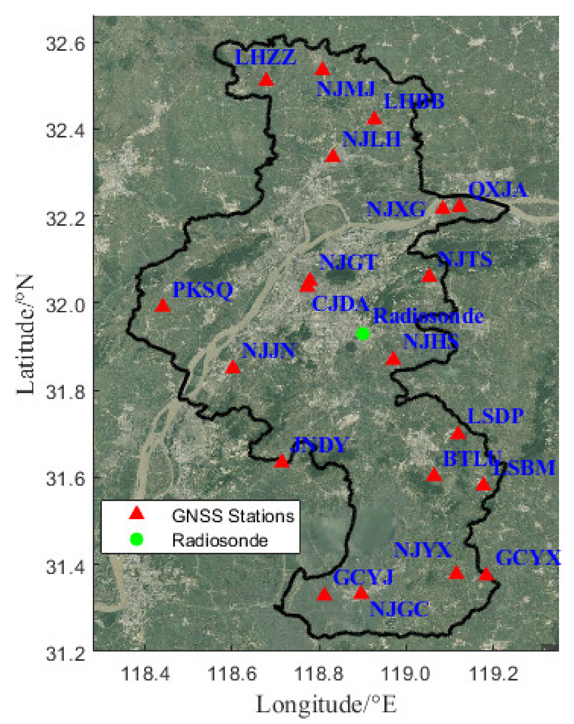
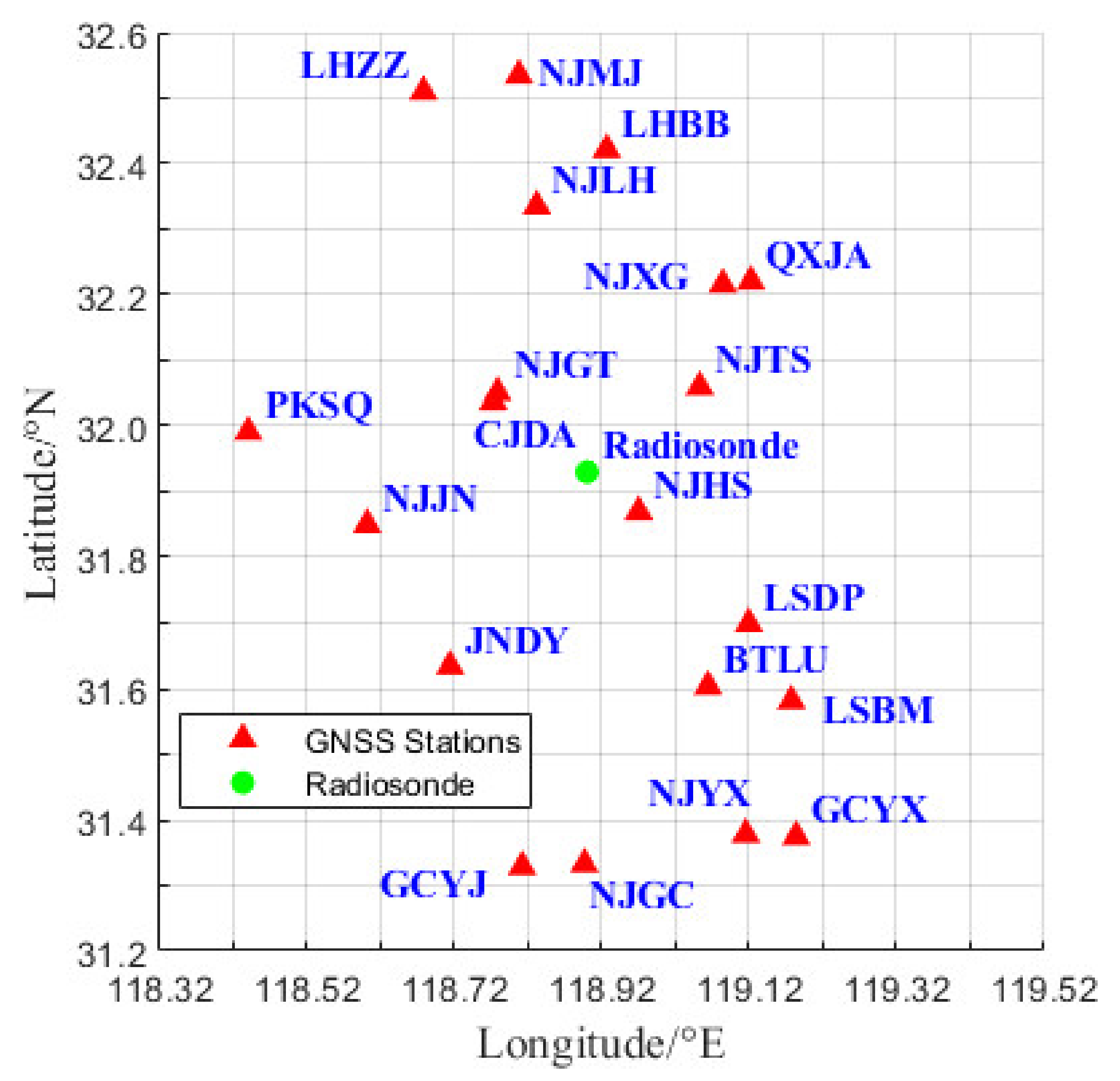
3.1. Study Area and Data Preprocessing

Nanjing, China, is the selected study area (latitude: 31.2°N–32.6°N, longitude: 118.3°E–119.3°E). As shown in Figure 5, 20 GNSS stations (NJCORS network) and 1 RS station (ID code: 58238) exist in the experimental coverage area. The 20 uniformly distributed stations (mean distance between stations is approximate 25 km) can continuously provide GNSS observations, while the RS can provide accurate WV profiles and ground temperature. These profiles can be regarded as both prior information and the truth value. The former is used as the initial value for the tomographic equation, while the latter is used as the truth value for the tomographic algorithm verification. To evaluate the performances and applicability of the tomographic approaches, we collected the GNSS observations from NJCORS in two periods under different weather conditions, 1 July to 3 July (day-of-year (DOY): 182 to 184) and 1 September to 3 September (DOY: 244 to 246). The weather conditions in the above two periods are shown in

Table 1. Two periods and their day-of-years (DOY)s and weather conditions.

Period	Day-of-Year (DOY)	Weather Conditions
1	182–184	clear or cloudy
2	244–246	rain

.

The six-day GNSS observations from 20 sites are processed by the double-difference model in the GAMIT software (version 10.71) [38]. Regarding the processing strategy, we use the International GNSS Service (IGS) final precise ephemeris and precise satellite clock correction to mitigate the satellite orbit and clock biases and set a sampling rate of 30 s and cut-off elevation angle of 10° for GNSS observations. After the above process, we can obtain the PWV and ZWD products of each station. The SWD in all signal directions can be then retrieved using Equation (4).

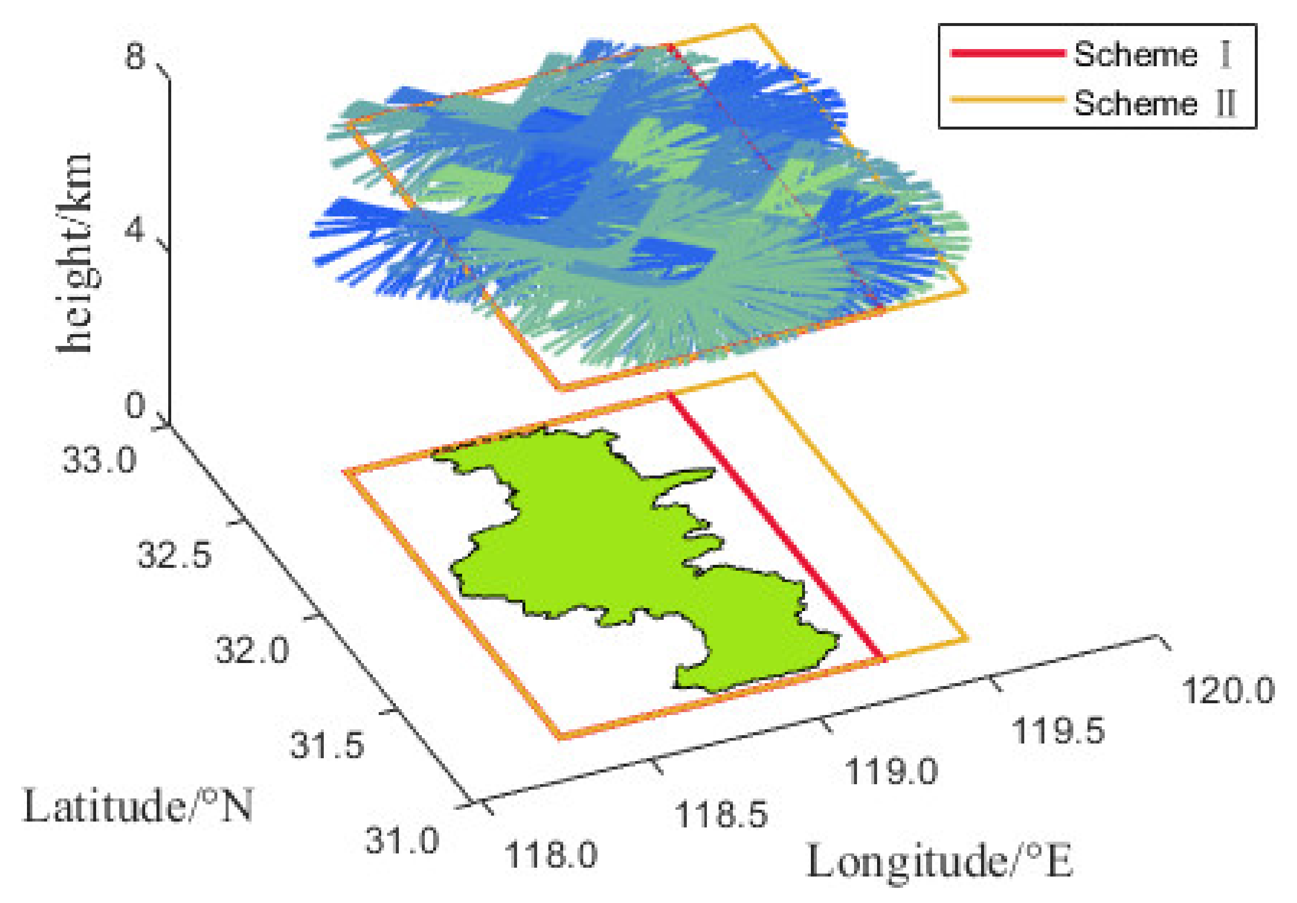
3.2. Gridding Schemes

Before the determination of the appropriate gridding scheme, we need to define the boundaries of the tomographic region, including the ground and top boundaries. A plane with a height of 8 km is selected as the top boundary according to the principle proposed by Yao et al. [23]. The “tropospheric cuboid” (i.e., tropospheric zone) is divided into 10 layers from bottom to top with thicknesses of 0.5, 0.5, 0.7, 0.7, 0.7, 0.9, 0.9, 0.9, 1.1, and 1.1 km. In general, the ground boundary only needs to cover the entire interest area, which excludes a large number of effective signals. The proposed improved method enables a larger ground boundary, although it may lead to more null-ray-passed voxels. Therefore, we gather the intersections of all receiver signal lines and 8-km-high tropopause at DOY 182, 2019 (1 July), presented in Figure 6. The general ground boundary (scheme I) only covers the experimental area, while the expanded boundary (scheme II) is extended by 0.25° in the longitude direction with respect to the general boundary. Compared to those in scheme I, the statistics in

Table 2. Total numbers and utilization rates of the GNSS signals for the two schemes.

Scheme	Total Number	Utilization Rate
I	1,443,492	93.56%
II	1,520,621	98.57%

show that the total number and utilization rate of the effective signal in scheme II are increased by 77,129 and 5.01%, from 1,443,492 and 93.56% to 1,520,621 and 98.57%, respectively. This reveals that scheme II is more suitable for this experiment than scheme I. Hence, we use scheme II for the ground boundary.

As shown in Figure 7, we set an interval of 0.1° in both longitude and latitude directions to grid the research area, which yields a 12 × 14 grid surface layer. By combining vertical layering strategies, the whole tropospheric cuboid is discretized into 12 × 14 × 10 independent voxels.

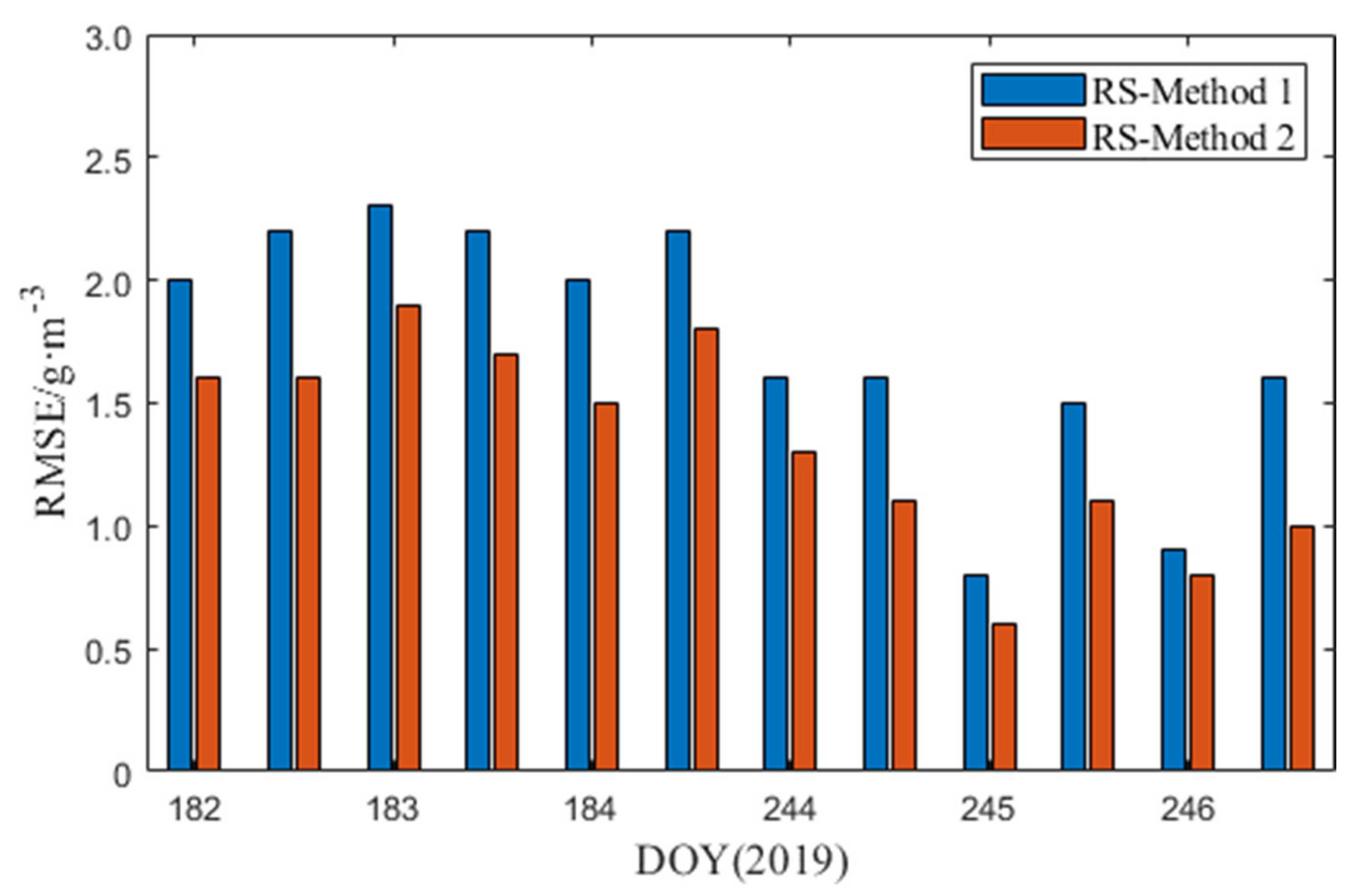
3.3. Validation of the Optimized Tomographic Method

We use two strategies for tomographic experiments, the conventional method (Method 1; Section 2.3), which introduces three constraints for the tomographic solution, and the improved method (Method 2) proposed is this paper (Section 2.4), which does not impose empirical constraints but only considers ray-passed voxels for the tomographic solution. Using the two methods, the experiments are carried out in the tomographic zone shown in Section 3.2 during the two periods mentioned in Section 3.1 based on the gridding scheme descried in the last section.

The RS provides the most accurate WV products, usually assumed as truth to validate the quality of tomographic results. Another resource of WV data, the European Center for Medium-Range Weather Forecast (ECMWF) products, is often used as a reference in the verification of the performance of the tomographic method. However, our previous study [25] has demonstrated that the 3D WV products derived from ECMWF cannot match the products acquired by the RS. Thus, the WV products derived from ECMWF are not used as a reference in this study. In this experiment, the mean absolute error (MAE), root mean square error (RMSE), and bias are used as statistical quantities to evaluate the quality of the tomographic results.

As RS balloons are launched twice (at UTC 00:00 and 12:00) per day, we can obtain two-epoch accurate WV profiles daily for tomographic method comparison. Meanwhile, the WV profiles for the location of the RS are calculated using the GNSS WV tomographic technique based on the two aforementioned methods at the corresponding epoch of RS balloons launched, respectively. Figure 8 shows the RMSE statistics of the WV profile differences between the above methods and RS data over the test period. The RMSEs of Method 2 are smaller than those of Method 1 at all test epochs. The RMSEs of Method 1 and Method 2 at DOY 244–246, 2019 (rainy weather), are better than those at DOY 182–184, 2019 (rainless weather). Besides, the statistics in

Table 3. Statistics of the tomography accuracy with respect to the RS method during a rainless period and a rainy period (g/m3).

	Root Mean Square Error (RMSE) (Rainless)	RMSE (Rainy)
RS–Method 1	2.2	1.3
RS–Method 2	1.7	1.0

show that Method 2 has higher accuracy in both rainy and rainless weather compared with Method 2, indicating again that Method 2 exhibits better performance and applicability with respect to Method 1.

We selected the two epochs with the minimum and maximum RMSEs for both Method 1 and Method 2 and compare the WV profiles of the two tomographic methods and RS method at these epochs in Figure 9. As shown in Figure 9a, the WV profiles obtained using Method 1 and Method 2 are in good agreement with that obtained using the RS data at UTC 00:00 DOY 245, 2019. Nevertheless, Figure 9b shows that the WV profiles generated using the two tomographic methods do not match well with the WV profile obtained using the RS at UTC 00:00 DOY 183, 2019. Thus, the two tomographic strategies exhibit higher performances in the rainy period than in the rainless period (recall Figure 8 and Table 3). Figure 9 shows that the vertical distributions of WV appear more even during the rainy day than during the rainless day. As shown in Figure 9b, the tropospheric WV exhibits a large change at heights below 4 km and a small change at heights above 4 km. This indicates that the moisture content near the ground is abundant but irregular on clear days. According to the study by Zhang et al. [24], the WV with an even distribution is beneficial for good tomographic results obtained by the GNSS WV tomographic technique. Thus, the GNSS tomographic algorithm has a higher performance in the rainy period than in the clear period. In addition, owing to these interference constraints, the WV profile obtained by Method 1 is closer to the conventional WV distribution than that obtained by Method 2, which can be attributed to the low performance of Method 1 during the rainless days.

To further evaluate the performances of the two tomographic methods, we calculate the mean bias, MAE, and RMSE between the RS and above methods; the numerical results are listed in

Table 4. Statistical comparison of the RS method and two methods in the experiment period (g/m³).

	Bias	Mean Absolute Error (MAE)	RMSE
RS–Method 1	−1.2	1.3	1.8
RS–Method 2	−0.8	0.9	1.3

. The RS data comparison shows that the mean RMSE of the proposed method (Method 2) is 1.3 g/m³, while that of the conventional method (Method 1) is 1.8 g/m³, which indicates that the accuracy of the tomographic method is increased by 27.8%. The MAE and bias of RS–Method 2 are 0.9 g/m³ and −0.8 g/m³, while those of RS–Method 1 are 1.3 g/m³ and −1.2 g/m³, respectively. These accuracy performance indicators show that Method 2 provides better tomographic results than those obtained by Method 1. Notably, the biases of RS–Method 1 and RS–Method 2 are negative, which reveals that the GNSS WV tomography usually overestimates the WV content of the troposphere. Accordingly, Figure 9a shows that the WV density obtained by the GNSS tomographic technique (blue and red lines) is higher than that obtained by the RS method (black lines) at almost all altitudes.

For a more intuitive comparison of the two methods in terms of altitude, the RMSE and relative error for different heights during the test period are shown in Figure 10. The RMSE and relative error of Method 2 are smaller than those of Method 1, particularly in the lower layer of the troposphere. Moreover, Figure 10a shows that the RMSEs of the two methods initially increased, and then they decreased with the altitude. The inflection point is observed at a height of approximately 1 km. This shows that the WV distributed at the height of approximately 1 km frequently varies, compared to other locations, so that the GNSS tomographic method cannot be used to estimate it well. Figure 10b shows that the relative errors of the different methods exhibit the same trend, i.e., they increase with the altitude. Owing to the low WV contents in the upper layers, even a small diversion would cause a large relative error. This may explain the results in Figure 10b.

4. Conclusions

We presented a new tomographic method based on the optimized voxel (only included ray-passed voxels). Besides, the new tomographic applied no empirical constraints but imposed vertical constraints originate from GNSS-derived precipitable water vapor (PWV). A conventional tomographic method that introduced three types of constraints (i.e. horizontal, vertical, and boundary constraints) is used as a comparison. We use the two tomographic methods to reconstruct the 3D water vapor (WV) fields in Nanjing during two selected periods with different weather conditions. The performance and reliability of the proposed tomographic method were validated by radiosonde (RS) data. Compared to the conventional method, the accuracy of the tomographic method is increased by 27.8% in terms of RMSE. For a large GNSS network, the proposed method is interference-free from empirical constraints and exhibits a better agreement with the RS method than the conventional method, particularly on clear days with largely changed moisture contents. Therefore, for the large GNSS network, the optimized method can be used to overcome the ill-posed problem caused by sparsely distributed stations, instead of using massive constraints to bias the tomographic results. Regarding the voxels eliminated by the proposed method, we simply use interpolation to obtain their WV densities using the voxels with WV values around them. Further studies can be carried out to evaluate the proposed tomographic method in different locations and different periods.

References

1. Bevis, M.; Businger, S.; Herring, T.A.; Rocken, C.; Anthes, R.A.; Ware, R.H. GPS meteorology: Remote sensing of atmospheric water vapor using the Global Positioning System. J. Geophys. Res. Atmos. 1992, 97, 15787–15801. [Google Scholar] [CrossRef]
2. Tregoning, P.; Boers, R.; O’Brien, D.; Hendy, M. Accuracy of absolute precipitable water vapor estimates from GPS observations. J. Geophys. Res. Atmos. 1998, 103, 28701–28710. [Google Scholar] [CrossRef]
3. Li, X.; Zus, F.; Lu, C.; Dick, G.; Ning, T.; Ge, M.; Wickert, J.; Schuh, H. Retrieving of atmospheric parameters from multi-GNSS in real time: Validation with water vapor radiometer and numerical weather model. J. Geophys. Res. Atmos. 2015, 120, 7189–7204. [Google Scholar] [CrossRef] [Green Version]
4. Li, X.; Zus, F.; Lu, C.; Ning, T.; Dick, G.; Ge, M.; Wickert, J.; Schuh, H. Retrieving high-resolution tropospheric gradients from multiconstellation GNSS observations. Geophys. Res. Lett. 2015, 42, 4173–4181. [Google Scholar] [CrossRef] [Green Version]
5. Li, X.; Dick, G.; Ge, M.; Heise, S.; Wickert, J.; Bender, M. Real-time GPS sensing of atmospheric water vapor: Precise point positioning with orbit, clock, and phase delay corrections. Geophys. Res. Lett. 2014, 41, 3615–3621. [Google Scholar] [CrossRef] [Green Version]
6. Wang, X.; Wang, X.; Dai, Z.; Ke, F.; Cao, Y.; Wang, F.; Song, L. Tropospheric wet refractivity tomography based on the BeiDou satellite system. Adv. Atmos. Sci. 2014, 31, 355–362. [Google Scholar] [CrossRef]
7. Yao, Y.; Shan, L.; Zhao, Q. Establishing a method of short-term rainfall forecasting based on GNSS-derived PWV and its application. Sci. Rep. 2017, 7, 1–11. [Google Scholar] [CrossRef]
8. Rohm, W.; Yuan, Y.; Biadeglgne, B.; Zhang, K.; Le Marshall, J. Ground-based GNSS ZTD/IWV estimation system for numerical weather prediction in challenging weather conditions. Atmos. Res. 2014, 138, 414–426. [Google Scholar] [CrossRef]
9. Zhao, Q.; Liu, Y.; Ma, X.; Yao, W.; Yao, Y.; Li, X. An improved rainfall forecasting model based on GNSS observations. IEEE Trans. Geosci. Remote Sens. 2020, 58, 4891–4900. [Google Scholar] [CrossRef]
10. Torres, B.; Cachorro, V.E.; Toledano, C.; Ortiz de Galisteo, J.P.; Berjón, A.; De Frutos, A.; Bennouna, Y.; Laulainen, N. Precipitable water vapor characterization in the Gulf of Cadiz region (southwestern Spain) based on Sun photometer, GPS, and radiosonde data. J. Geophys. Res. Atmos. 2010, 115, D18. [Google Scholar] [CrossRef] [Green Version]
11. Gurbuz, G.; Jin, S. Long-time variations of precipitable water vapour estimated from GPS, MODIS and radiosonde observations in Turkey. Int. J. Climatol. 2017, 37, 5170–5180. [Google Scholar] [CrossRef]
12. Li, Z.; Muller, J.P.; Cross, P. Comparison of precipitable water vapor derived from radiosonde, GPS, and Moderate-Resolution Imaging Spectroradiometer measurements. J. Geophys. Res. Atmos. 2003, 108, D20. [Google Scholar] [CrossRef]
13. Liu, C.; Zheng, N.; Zhang, K.; Liu, J. A new method for refining the GNSS-derived precipitable water vapor map. Sensors 2019, 19, 698. [Google Scholar] [CrossRef] [Green Version]
14. Dai, A.; Wang, J.; Ware, R.H.; Van Hove, T. Diurnal variation in water vapor over North America and its implications for sampling errors in radiosonde humidity. J. Geophys. Res. Atmos. 2002, 107, D10. [Google Scholar] [CrossRef] [Green Version]
15. Alshawaf, F.; Fuhrmann, T.; Knöpfler, A.; Luo, X.; Mayer, M.; Hinz, S.; Heck, B. Accurate estimation of atmospheric water vapor using GNSS observations and surface meteorological data. IEEE Trans. Geosci. Remote Sens. 2015, 53, 3764–3771. [Google Scholar] [CrossRef]
16. Chen, B.; Liu, Z. Voxel-optimized regional water vapor tomography and comparison with radiosonde and numerical weather model. J. Geod. 2014, 88, 691–703. [Google Scholar] [CrossRef]
17. Dong, Z.; Jin, S. 3-D water vapor tomography in Wuhan from GPS, BDS and GLONASS observations. Remote Sens. 2018, 10, 62. [Google Scholar] [CrossRef] [Green Version]
18. Flores, A.; Ruffini, G.; Rius, A. 4D tropospheric tomography using GPS slant wet delays. Ann. Geophys. 2000, 18, 223–234. [Google Scholar] [CrossRef]
19. Perler, D.; Geiger, A.; Hurter, F. 4D GPS water vapor tomography: New parameterized approaches. J. Geod. 2011, 85, 539–550. [Google Scholar] [CrossRef] [Green Version]
20. Rohm, W. The ground GNSS tomography-unconstrained approach. Adv. Space Res. 2013, 51, 501–513. [Google Scholar] [CrossRef]
21. Rohm, W.; Zhang, K.; Bosy, J. Limited constraint, robust Kalman filtering for GNSS troposphere tomography. Atmos. Meas. Tech. 2014, 7, 1475–1486. [Google Scholar] [CrossRef] [Green Version]
22. Yang, F.; Guo, J.; Shi, J.; Zhao, Y.; Zhou, L.; Song, S. A new method of GPS water vapor tomography for maximizing the use of signal rays. Appl. Sci. 2019, 9, 1446. [Google Scholar] [CrossRef] [Green Version]
23. Yao, Y.; Zhao, Q. A novel, optimized approach of voxel division for water vapor tomography. Meteorol. Atmos. Phys. 2017, 129, 57–70. [Google Scholar] [CrossRef]
24. Zhang, B.; Fan, Q.; Yao, Y.; Xu, C.; Li, X. An improved tomography approach based on adaptive smoothing and ground meteorological observations. Remote Sens. 2017, 9, 886. [Google Scholar] [CrossRef] [Green Version]
25. Zhao, Q.; Yao, W.; Yao, Y.; Li, X. An improved GNSS tropospheric tomography method with the GPT2w model. GPS Solut. 2020, 24, 1–13. [Google Scholar] [CrossRef]
26. Zhao, Q.; Yao, Y.; Cao, X.; Zhou, F.; Xia, P. An optimal tropospheric tomography method based on the multi-GNSS observations. Remote Sens. 2018, 10, 234. [Google Scholar] [CrossRef] [Green Version]
27. Zhao, Q.; Zhang, K.; Yao, Y.; Li, X. A new troposphere tomography algorithm with a truncation factor model (TFM) for GNSS networks. GPS Solut. 2019, 23, 64. [Google Scholar] [CrossRef]
28. Zhang, W.; Zhang, S.; Nan, D.; Pengxu, M. An improved tropospheric tomography method based on the dynamic node parametrized algorithm. Acta Geodyn. Geomater. 2020, 17, 191–206. [Google Scholar] [CrossRef]
29. Zhang, W.; Zhang, S.; Ding, N.; Zhao, Q. A tropospheric tomography method with a novel height factor model including two parts: Isotropic and anisotropic height factors. Remote Sens. 2020, 12, 1848. [Google Scholar] [CrossRef]
30. Zhao, Q.; Li, Z.; Yao, W.; Yao, Y. An improved ridge estimation (IRE) method for troposphere water vapor tomography. J. Atmos. Sol.-Terr. Phys. 2020, 207, 105366. [Google Scholar] [CrossRef]
31. Saastamoinen, J. Atmospheric correction for the troposphere and stratosphere in radio ranging satellites. Bull. Géodésique 1972, 15, 247–251. [Google Scholar]
32. Wang, X.; Zhang, K.; Wu, S.; Fan, S.; Cheng, Y. Water vapor-weighted mean temperature and its impact on the determination of precipitable water vapor and its linear trend. J. Geophys. Res. Atmos. 2016, 121, 833–852. [Google Scholar] [CrossRef]
33. Rohm, W.; Bosy, J. Local tomography troposphere model over mountains area. Atmos. Res. 2009, 93, 777–783. [Google Scholar] [CrossRef]
34. Gradinarsky, L.P.; Jarlemark, P. Ground-based GPS tomography of water vapor: Analysis of simulated and real data. J. Meteorol. Soc. Jpn. 2004, 82, 551–560. [Google Scholar] [CrossRef] [Green Version]
35. Nilsson, T.; Gradinarsky, L. Water vapor tomography using GPS phase observations: Simulation results. IEEE Trans. Geosci. Remote Sens. 2006, 44, 2927–2941. [Google Scholar] [CrossRef]
36. Ding, W.; Wang, J.; Rizos, C.; Kinlyside, D. Improving adaptive Kalman estimation in GPS/INS integration. J. Navig. 2007, 60, 517–529. [Google Scholar] [CrossRef] [Green Version]
37. Groves, P.D. Principles of GNSS, Inertial, and Multisensor Integrated Navigation Systems; Artech House: London, UK, 2013. [Google Scholar]
38. Li, G.; Wang, H. Using GAMIT to derive the precipitabel water vapor. In Proceedings of the 2010 International Conference on Multimedia Technology, Ningbo, China, 29–31 October 2010; pp. 1–4. [Google Scholar]
Figure 1. Principle of water vapor (WV) tomography with Global Navigation Satellite System (GNSS) observations.
Remotesensing 12 02306 g001
Figure 2. Ground projection distance (ab) of the segment (ac) between the receiver (a) and point (c). The point (c) is the intersection of the ray and tropopause.
Remotesensing 12 02306 g002
Figure 3. Voxel optimization process. (a) All voxels in the tomographic zone. (b) All voxels and visual rays from three sites. (c) Voxels through which rays pass.
Remotesensing 12 02306 g003
Figure 4. Precipitable WV (PWV) constraints imposed upon the tomographic equation.
Remotesensing 12 02306 g004
Figure 5. Experiment area, including 20 GNSS stations (red triangles) and 1 radiosonde (RS) station (green circle).
Remotesensing 12 02306 g005
Figure 6. Intersection of the ray and 8-km-high tropopause. In scheme I, a general tomographic horizontal boundary covering only the Nanjing area is used, while in scheme II, the optimal horizontal boundary including the most signals is used.
Remotesensing 12 02306 g006
Figure 7. Horizontal grid strategy. The Nanjing area is divided by a 12 × 14 grid in the horizontal domain (14 in the latitudinal direction, 12 in the longitudinal direction). The horizontal resolution is 0.1° in both the latitude and longitude directions.
Remotesensing 12 02306 g007
Figure 8. Statistics of the root mean square error (RMSE) differences for RS–Method 1 and RS–Method 2 at 00:00 and 12:00 UTC in the period of DOY 182–184, 2019, and DOY 244–246, 2019.
Remotesensing 12 02306 g008
Figure 9. WV profiles obtained by the different tomographic methods and RS method at UTC 00:00 DOY 245, 2019 (a), which is the best WV profile of the experiment epochs, while the worst WV profile is at UTC 00:00 DOY 183, 2019 (b).
Remotesensing 12 02306 g009
Figure 10. RMSEs (a) and relative errors (b) at different altitudes obtained using the two tomographic methods during the experiment period.
Remotesensing 12 02306 g010