Technical Note

Analysis of UAS Flight Altitude and Ground Control Point Parameters on DEM Accuracy along a Complex, Developed Coastline

1
Department of Civil, Environmental, and Ocean Engineering, Stevens Institute of Technology, Hoboken, NJ 07030, USA
2
Maritime Research Institute Netherlands, 6708 PM Wageningen, The Netherlands
*
Author to whom correspondence should be addressed.
Remote Sens. 2020, 12(14), 2305; https://doi.org/10.3390/rs12142305
Submission received: 4 June 2020 / Revised: 14 July 2020 / Accepted: 15 July 2020 / Published: 17 July 2020
(This article belongs to the Special Issue UAV Application for Monitoring Coastal Morphology)

Abstract

:
Measuring beach topography accurately and with high spatial resolution is an important aspect of coastal management and is crucial for understanding changes in beach morphology, especially along complex, three-dimensional shorelines. Traditional methods of beach surveying even at high resolution are insufficient to measure the complex, dynamic behavior along these coasts. This study investigates the optimization of Unmanned Aerial Systems Structure from Motion (UAS-SfM) data acquisition methodology with regard to flight altitude and the configuration and amount of ground control points (GCPs). A sensitivity analysis was performed to determine the UAS and GCP characteristics that produce the most accurate digital elevation model (DEM). First, an evaluation of the UAS-SfM technique was performed and proved advantageous over traditional surveying techniques with regard to efficiency, automation, ease of use, and repeatability. The results of the sensitivity analysis showed the highest (116 m) flight altitude evaluated was the most accurate and required the least amount of survey and processing time. The optimal configuration of GCPs was determined to be (1) in the corners of the study site, (2) at high and low elevations within the study site, and (3) with sufficient cross-shore and alongshore coverage. Finally, it was found that 15 GCPs produced the best results, but that as few as 11 GCPs could be used without any significant loss in accuracy. It was also observed that fewer (≈7–9) well-placed GCPs in the optimal configuration produced the same magnitude of error as using more (15) poorly placed GCPs. Based on these results, a set of recommendations for conducting UAS-SfM surveys along complex, three-dimensional, developed coastlines is presented.

Graphical Abstract

1. Introduction

The quantification of beach topography is important for understanding morphological evolution, monitoring beach nourishment projects, assessing storm-induced sediment transport, calculating rates of change, and more [1]. It is widely recognized as being significant, as beaches have direct and indirect impacts on ecosystems, the economy, recreation, and a wide variety of professions and lifestyles. In particular, understanding coastal processes, one of the foundations of coastal research, often relies on the topographic mapping of complex beach morphology [1]. The effectiveness of coastal management is strongly dependent on the accuracy and resolution of beach topography on both spatial and temporal scales; in many cases, topographic surveys need to be conducted regularly so that short-term trends and local changes in morphology can be identified and measured. The significance of having accurate maps increases at anthropogenically influenced coasts, i.e., where shore perpendicular structures such as groins exist. Typically, the dimensionality of beach morphology increases near coastal structures as they often induce erosional and accretional features such as scarps, localized hotspots, and/or other three-dimensional (3D) features that may not exist in uninterrupted or natural areas of beach. In order to capture these localized 3D features, modern surveying techniques such as an Unmanned Aerial System (UAS) equipped with a camera coupled with advanced image processing tools such as Structure from Motion (SfM) offer significant advantages as compared to traditional beach surveying methods. The objectives of this study are to highlight the results of analyses regarding the influence of UAS flight altitude and ground control point (GCP) amount and configuration on survey error, and to provide guidance on the optimal UAS and GCP survey characteristics for complex beach systems.

1.1. Background

A variety of surveying methods exist for mapping beach topography and quantifying volumetric changes [1], including spot measurements, walking measurements, and LiDAR (light detection and ranging). The most commonly used or ‘traditional’ method of measuring beach topography is to survey cross-shore beach profiles spanning from the dune or upland area to the swash zone using a real-time kinematic global positioning system (RTK GPS). Generally, the RTK GPS receiver is attached to a backpack, survey pole, or All-Terrain Vehicle (ATV), and numerous cross-shore profile lines are transgressed at established spacings. The major advantage of utilizing a survey pole and taking spot measurements is that the measurements are highly accurate (vertical heights and position accuracies of 0.01 m are attainable); however, this method is labor intensive, and large areas can only be sampled sparsely and infrequently [2]. A more efficient method (relatively) of collecting RTK GPS data involves the surveyor wearing an RTK GPS backpack and walking the profile lines. Vertical errors on the order of 0.052 m and above [3] have been found using this method as a result of sinking into the sand, poor walking posture, tilting while walking uphill or downhill, and more. This occurrence is displayed in Figure 1, in which a surveyor walking with an RTK GPS backpack is sinking into the sand and demonstrating tilted posture while surveying a cross-shore profile. The efficiency of RTK GPS surveys can be improved by mounting the RTK GPS to an ATV; however, similar sources of error are introduced.
Regardless of the method used to collect profile data, additional errors are introduced as the area between profile lines needs to be interpolated. If the data itself already have significant errors, this interpolation can lead to a false representation of the true morphology, even on simple flat beaches. The potential for significant error is even higher on beaches containing important 3D features such as beach cusps and/or localized erosion/accretion. In such a case, difficulties frequently arise when attempting to select which 2D cross-shore profile line is the most representative of the 3D beach in its local vicinity [2]. Additionally, in general, the magnitude of error increases as the dimensionality of the beach becomes more complex. For example, the morphology near man-made coastal structures is typically 3D and therefore requires a higher resolution survey to accurately measure the true morphology.
A high-precision and high-resolution approach to measuring beach topography is light detection and ranging, or LiDAR. LiDAR is a laser-based active remote sensing survey technique that can accurately measure large amounts of topographic data via airborne, vehicular, or ground-based platforms. It is possible to obtain measurements of terrain surfaces with an accuracy of 0.012 m using terrestrial LiDAR [4]. However, the drawbacks of LiDAR, which include high costs and difficulty of use, make it unusable or impractical for many cases. Mobile LiDAR systems such as airborne and vehicular LiDAR allow the rapid coverage of large areas; however, they typically demand significant resources for deployment [5], result in massive datasets that require intensive post-processing and as a result can be prohibitively expensive. Stationary ground-based LiDAR systems are cheaper and result in more manageable datasets that require less processing; however, they need to be moved multiple times to cover large areas and frequently contain blind spots where geomorphic features block the view field.
Recent advances in UAS technology, cameras, and associated software have made the process of creating realistic 3D topographic models easier and more accurate than ever before, and at significantly less cost than LiDAR. UAS for beach topography has become increasingly popular due to its high spatial resolution, low cost, ease of use, automation, and repeatability [6]. When 2D UAS images are coupled with the SfM algorithm, a photogrammetric range imaging technique, 3D topography maps, can be created and used to measure and monitor beach morphology [6]. The UAS-SfM method can generate dense point clouds and/or digital elevation models (DEMs), or a 3D representation of a terrain’s surface, with a vertical error of approximately 0.025 m [7]. This method can better and more efficiently capture 3D morphology as compared to traditional beach profiling methods as a result of the high spatial resolution and complete coverage of a site.
Table 1 describes four contemporary surveying systems and associated characteristics including cost, time of survey, efficiency, and accuracy. The data represents the systems in situ; all post-processing analysis and software considerations are excluded. In addition to the numerical parameters listed, it is important to consider the practicality of each system for the study site, access to the beach, maintenance, repeatability, ability to rapidly deploy, etc.
Of the systems presented in the table, the quadcopter UAS has the lowest cost and lowest time of survey, which makes it an ideal tool for the frequent monitoring of 3D surfaces, including beaches. In addition, the UAS is capable of producing very accurate surfaces with the assistance of a relatively high point density. Thus, the high spatial and temporal resolutions presented by the UAS-SfM method make it the quintessential tool for beach monitoring.

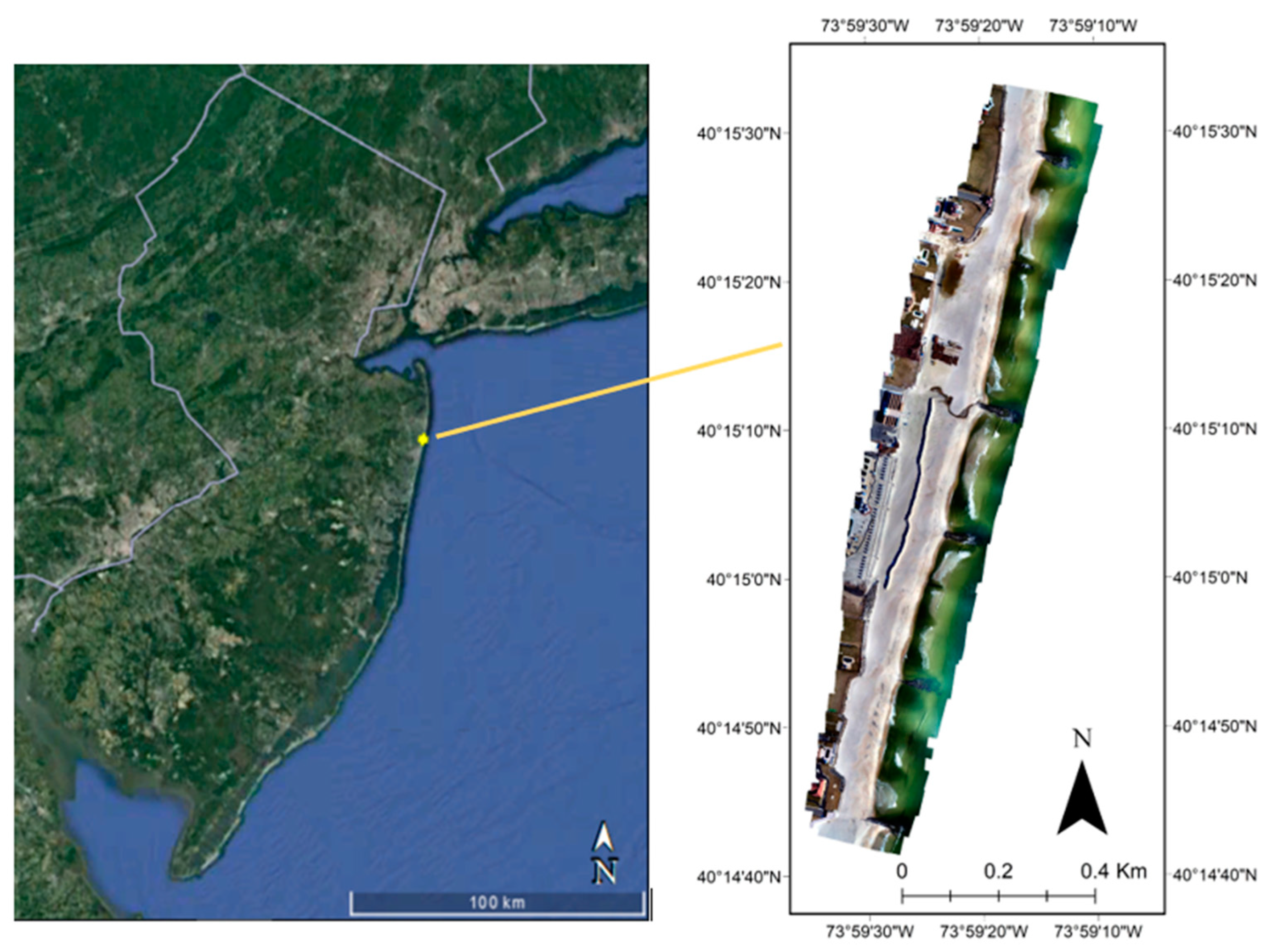
1.2. Site Description

The study site, shown in Figure 2, is located along the northern section of the New Jersey coastline in Deal, which spanned approximately 1.6 km alongshore and covered 0.12 km2 of dry beach.
Deal beach is a relatively narrow public beach that fronts a series of coastal bluffs, residential homes, and a beach club. This site was selected due to its highly modified shoreline and recent beach nourishment. Deal beach is an archetype of a modified beach, as it contains eight groins that make up a groin field. The primary function of the groins (shore-perpendicular rock structures) is to trap or slow down a percentage of longshore sediment transport to stabilize areas of vulnerable beach and lessen the impacts of erosion. The groins at Deal were designed and constructed prior to our modern understanding of their function [9] and therefore are too long and inappropriately spaced. As a result, they trap too much sediment transported by alongshore currents, which introduces significant erosion/accretion patterns and localized 3D features.
In addition to the early construction of groins, the beaches along the New Jersey coastline from Sandy Hook to Barnegat Inlet (which encompasses Deal) have been nourished since 1994 [10]. More recently, in 2012 during Hurricane Sandy, this section of coastline lost approximately 3.8 million cubic meters of sand. In response, the U.S. Army Corps of Engineers (USACE) carried out a beach nourishment project called the Sandy Hook to Barnegat Inlet Beach Erosion Control Project, in which they placed roughly 6 million cubic meters of sand over a 34 km stretch of New Jersey shoreline [10]. This project is significant, as it was the largest beach nourishment project ever performed by the USACE and at the time was the largest beachfill, in terms of volume, in the world [11]. This project was performed to completion in 2016 and has since been awarded additional nourishment contracts [10].
Simultaneous to the 2016 beach nourishment, multiple groins in Deal were notched to address the inappropriate groin field design. Groin notching is an uncommon method of attempting to reduce some of the less desirable effects of groins, such as significant erosion/accretion patterns, by removing a section of the structure in the swash zone. The objective is to increase the amount of sediment permitted to bypass the structure while still maintaining a stable shoreline position. Figure 3a,b provides an example of a notched groin and traditional groin at Deal beach, where the notch (removed groin section) is highlighted by a yellow box.
The result of the pre-existing groin field, beach nourishment, and groin notching is a complex beach system that ranges from nearly 2D to highly 3D over short spatial distances, and one that changes rapidly in response to relatively small changes in the wave climate. Deal beach is a prime example of a site that necessitates morphological monitoring in order to study the complex coastal processes driven by a variety of anthropogenic factors. Therefore, in order to understand this system, frequent high-resolution measurements such as those collected by UAS-SfM are required. In an effort to maximize the accuracy and efficiency of UAS surveys at Deal beach, a series of experiments were conducted to determine the optimal flight and ground control parameters for generating DEMs of the 3D yet fairly homogenous beach surface.

2. Materials and Methods

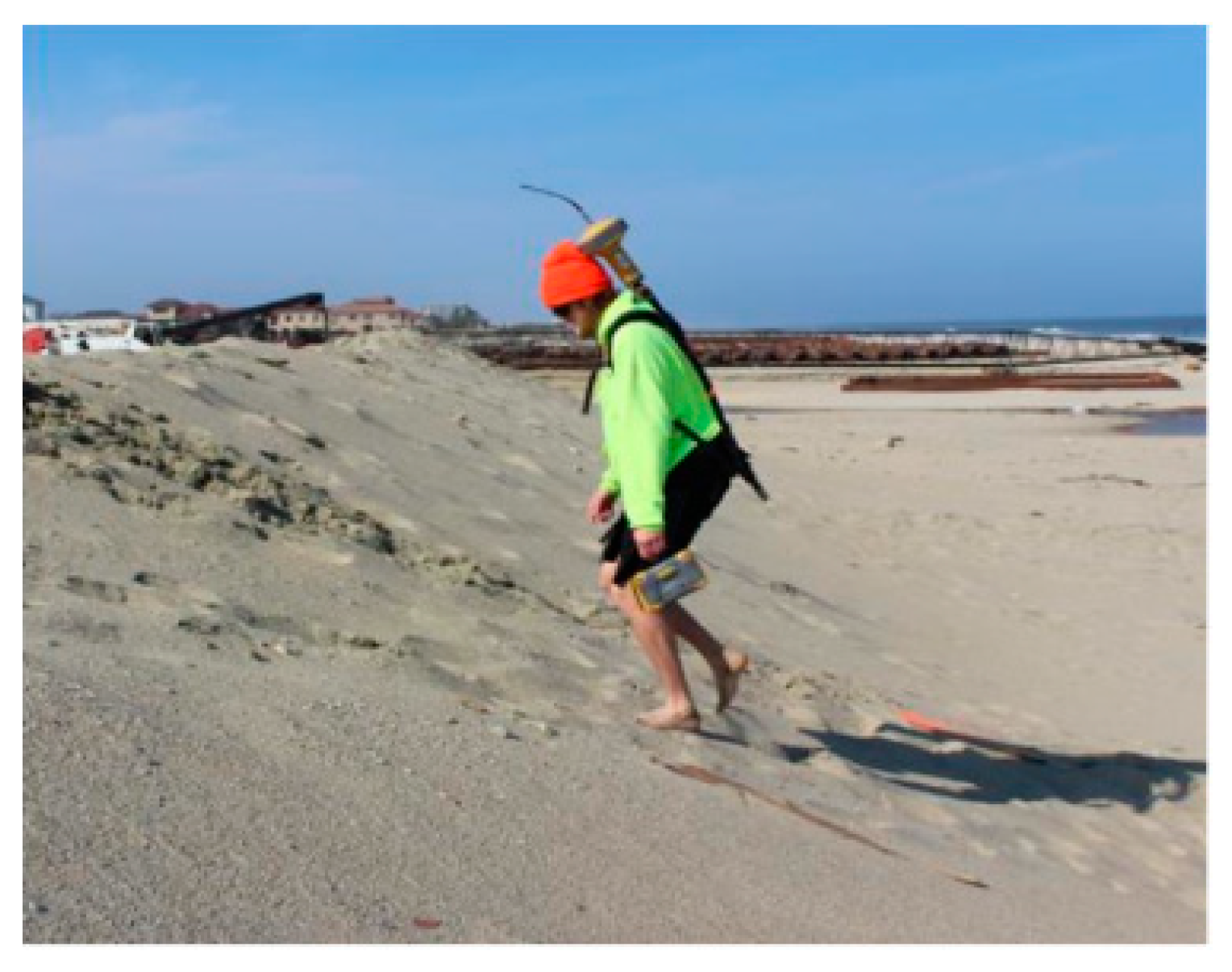
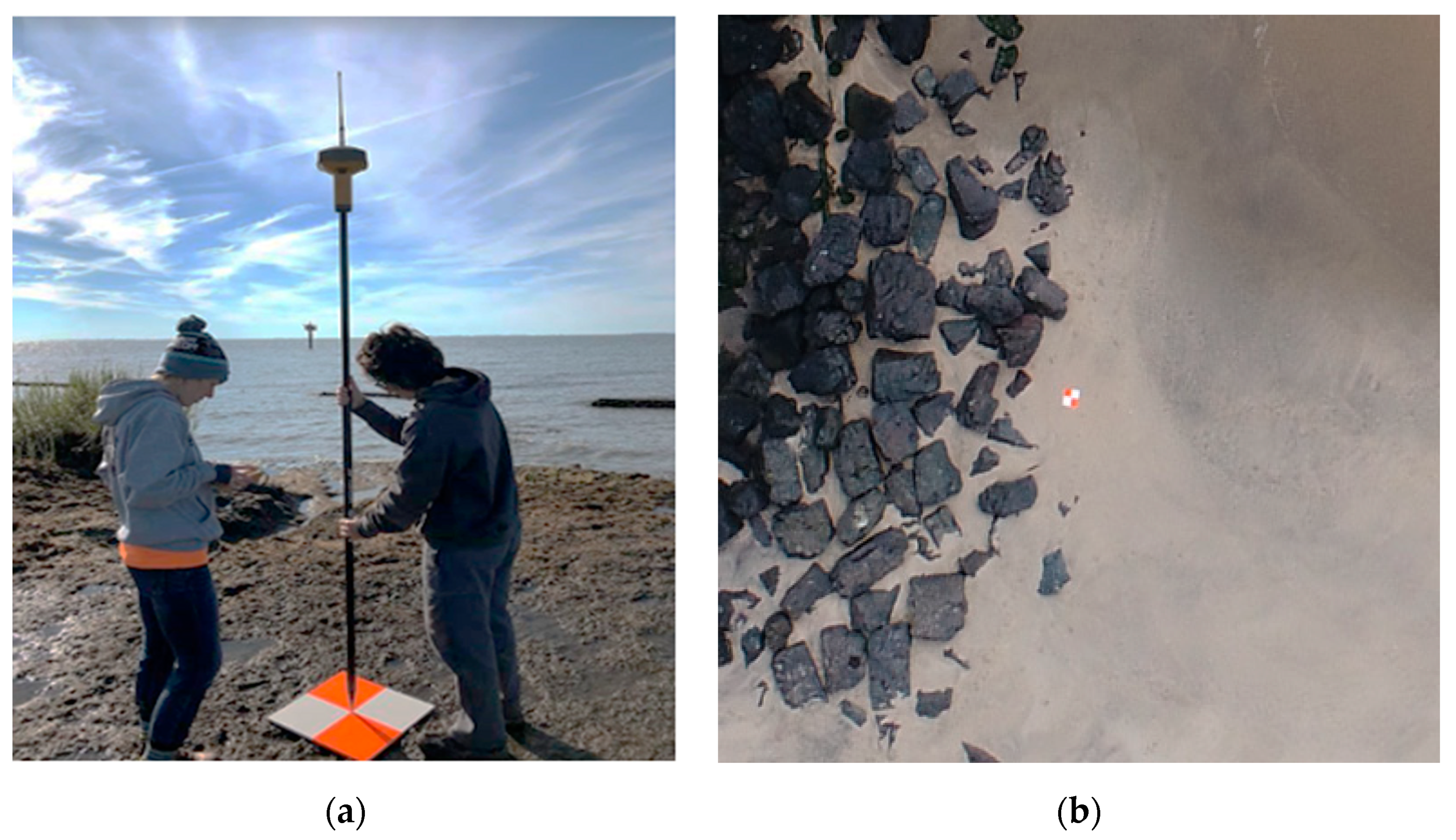
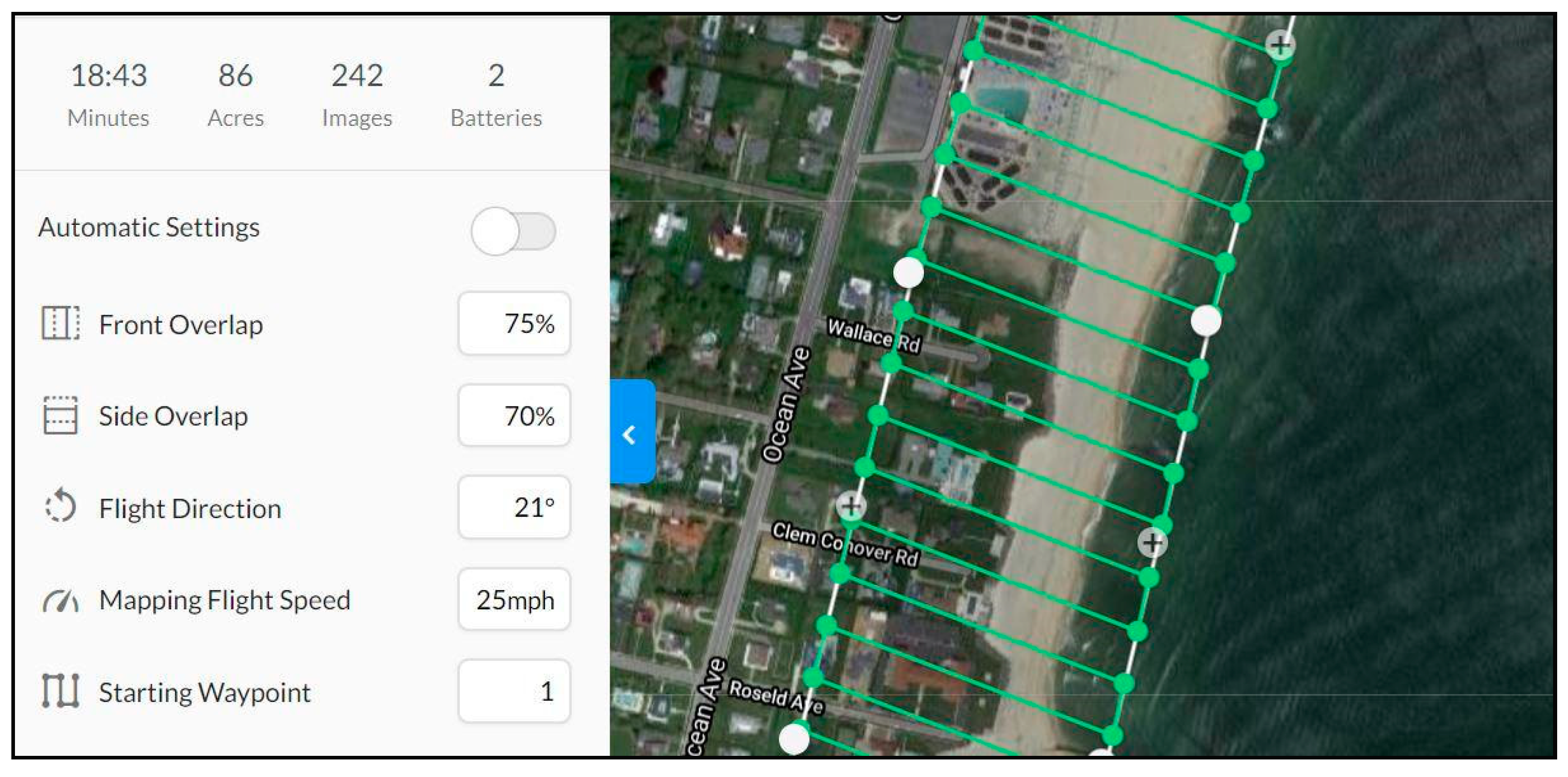
2.1. Equiptment and Survey Setup

A DJI Phantom 4 Pro UAS equipped with a frame camera was utilized for collecting the aerial imagery used in this project. The Phantom 4 Pro is a quadcopter that has a 3-axis (roll, pitch, yaw) gimbal for stabilization. It weighs 1388 g and has a diagonal size of 35 cm excluding the propellers. Attached is a 1 CMOS camera sensor that has 20 M effective pixels. The lens is a FOV 84° 8.8 mm/24 mm (35 mm format equivalent) that produces an image size of 4864 × 3648 pixels [12]. The UAS includes a handheld remote with a USB attachment for a smartphone, which was used to control the flights via the DroneDeploy iPhone app.
The flights conducted for this study complied with the United States Federal Aviation Administration (FAA) Part 107 UAS Operation regulations [13]. All flights were planned prior to deployment using DroneDeploy software. DroneDeploy allows the user to input desired survey area, flight altitude, flight direction, and front and side image overlap. The software automatically estimates the time of flight, the number of images that will be captured, and the number of batteries needed based on the input parameters. Once in the field and the connection is setup between the UAS and DroneDeploy app, the flight and image acquisition is executed autonomously following the predefined survey parameters. Figure 4 shows the DroneDeploy software planning screen in which the user can define flight parameters. The associated map provides an aerial view of the area with the flight lines, shown in green, that correspond to the parameters set in the user interface. The user can configure the survey area boundaries using this map.
The survey area boundary in the DroneDeploy map exceeds the area of interest, which is the dry beach; the total surveyed area covered approximately 0.25 km2 with a dry beach area of 0.12 km2. It is important for the survey boundary to exceed the area of interest for multiple reasons. In general, making the boundary larger than the area of interest ensures a sufficient amount of image overlap within the area of interest. This factor is especially important for beaches, as shoreline erosion/accretion can cause the beach to look dramatically different than that of the preloaded aerial. It is also important to be aware of the tidal range at the study site and to account for the uncertainty of the state of the tide in the preloaded aerial. With that, performing the UAS survey at low tide is ideal in order to capture the maximum area of dry beach. Specific to this site, expanding the survey area in the upland direction to the houses adds higher elevations and fixed 3D structures to the survey, which is helpful for the UAS-SfM technique since the dry beach is fairly homogenous.
When setting up the survey boundary, it is important to make sure that all GCPs are well within the boundary lines. A GCP is defined as a physically marked location or object whose positions are measured in reference to a known coordinate system, typically using RTK GPS spot measurements. GCPs can be placed targets, fixed landmarks, or anything stationary that can be seen clearly from an aerial image. Figure 5a,b shows a field measurement of a GCP using an RTK GPS spot measurement system and the typical view of a GCP from an UAS aerial image.
For this study, the GCPs utilized were orange and white checkerboard pattern targets that were approximately 0.6 m by 0.6 m. There were 21 GCP targets strategically placed throughout the dry beach area with intentions to achieve sufficient cross-shore and alongshore coverage. Since this area is along a heavily developed section of coast, there are residential homes and a beach club that are located directly upland of the beach (there are no dunes). Therefore, the GCPs could not be placed outside of the dry beach area, since access to the beach club or private properties was not provided. The GCP locations and elevations were surveyed with a Topcon GR-5 RTK GPS receiver system. The RTK receiver was attached to a 2 m survey pole and placed in the center of the GCP by one surveyor, and the handheld, which was operated by another surveyor, recorded the data points. For each GCP, three consecutive spot measurement points were recorded in effort to obtain a more precise value and proactively mitigate any missing or bad data. In post-processing, the measurements were quality controlled (any obvious outliers were removed), and the median value of the three measurements was used as the position of each GCP. According to the Topcon GR-5 operator’s manual, the receiver can achieve an RTK accuracy of 10 mm in the horizontal plane and 15 mm in the vertical plane [7]. Thus, the measured location of each GCP was extremely precise. The significance of obtaining accurate GCP positional data while using the UAS-SfM technique is immense and is detailed further in the following section.

2.2. Structure from Motion (SfM) Technique

The images taken using DroneDeploy were processed via the SfM technique in Agisoft Photoscan software (updated version renamed ‘Agisoft Metashape’). SfM is a photogrammetric range imaging technique that creates three-dimensional models from overlapping two-dimensional images taken from various positions [14]. SfM can produce dense point clouds through post-processing algorithms by matching thousands of features (“tie-points”) that are automatically detected in the multiple overlapping of 2D images. While the dense point clouds produced can be similar to that of LiDAR, SfM is advantageous because of its lower cost, automation, and ease of use [14]. UAS-SfM automatically solves the 3D location and orientation of each image; every time an image is captured, the corresponding 6 degrees of freedom (latitude, longitude, altitude, roll, pitch, yaw) are recorded. Camera characteristics such as focal point, calibration parameters, focal length, aperture, resolution, etc. are considered when solving, and all of the data are stored as an Exif (exchangeable image file format) for the reader [14]. The Photoscan software uses bundle adjustments to optimize the camera parameters and point feature networks to define a 3D surface using the least-squares errors method [15].
Initially, the UAS-SfM generated dense point cloud is aligned and oriented exclusively by the UAS-stored parameters in a relative ‘image-space’ coordinate system. In order to relate the model to a ‘real-world’ coordinate system, inexpensive UASs such as the DJI Phantom 4 Pro make use of GCPs.
GCPs are utilized by image processing software to (1) assign the resulting map to a real-world coordinate system, and (2) use their known precise positions to improve the accuracy of a map through georeferencing. Georeferencing is the process of taking digital images and adding positioning information so that mapping software can place the image in its real-world location [16]. It is important to note that the geographic coordinate system was the same for the RTK GPS field measurements and Agisoft Photoscan software; the projected horizontal coordinate system used was NAD 1983 State Plane New Jersey (US feet) and the vertical datum was NAVD88 (North American Vertical Datum).
Since the dense point cloud produced via UAS-SfM is corrected and aligned to the GCPs, the accuracy and reliability of the resulting information is strongly dependent upon the characteristics (mostly accuracy, amount, and placement) of the GCP system. Guidance on the number and placement of GCPs is inconsistent and varies greatly based on the survey objectives, the size and shape of the survey site, and other characteristics. This is particularly true for complex sites with such a high degree of image homogeneity. DroneDeploy recommends using between 4 and 10 GCPs distributed evenly over the surveyed area. It is also recommended that the GCPs be visible in a minimum of 4 images and that they are placed at the highest and lowest points of elevation to account for elevation changes on relatively flat surfaces [17]. Other recommendations related to the number of GCPs were reported by Agisoft Metashape [18] and Tahar [19] as between 10–15 and 8–9, respectively, and neither mentioned GCP placement. A report by Brunier, Fleury, Anthony, Gardel, and Dussouillez [20] did not recommend a specific number of GCPs but emphasized the importance of placing GCPs in the cross-shore direction and backshore area. Similarly, there is a lack of definitive guidance on flight altitude, which affects the spatial resolution, flight time, number of images, tie points, image reconstruction, and more [21]. For these reasons, an analysis was undertaken to identify the optimal GCP configuration and flight parameters for this study site.

3. Results

The characteristics that were evaluated are UAS flight altitude, amount of GCPs, and GCP configuration. As described above, 21 GCP targets were distributed throughout the dry beach area of 0.12 km2, and the total survey area of 0.25 km2 remained fixed for each flight. For some of the tests, a selected portion of the GCP targets were not used in georeferencing to fit the resulting surface, but were instead used as check points. Flights were conducted at three different elevations, but all flights had the same boundary and image overlap (frontlap—80%, sidelap—75%). A systematic approach was used whereby the influence of flight altitude was evaluated first. Then, the optimal altitude was used to investigate GCP configuration. Once the optimal configuration was identified, the influence of GCP number was considered.

3.1. UAS Flight Altitude

The three altitudes tested were 67 m, 91 m, and 116 m. These altitudes were chosen based on the FAA maximum allowed flight altitude of 120 m [13]. The highest altitude chosen was 116 m to provide some buffer between the 120 m allowable altitude. Then, the altitude was reduced by increments of approximately 25 m for the other two flights tested: 91 m and 67 m, respectively. Table 2 outlines the flight altitudes and corresponding in situ and processing parameters.
The fifth column displays the Ground Sampling Distance (GSD), which is directly related to the flight altitude and camera parameters. The GSD is defined as the distance between two consecutive pixel centers measured on the ground. The greater the GSD value, the lower the spatial resolution of the image and the less visible details [22]. A pixel projected onto the ground may or may not be perfectly square, so the GSD is represented by the greater of the following two equations, Equations (1) and (2):
G S D h = ( H S h ) ( c I h )
G S D w = ( H S w ) ( c I w )
where
  • H is the flight altitude (67, 91, 116 m)
  • Sh is sensor height (=8 mm for DJI Phantom 4 pro)
  • Sw is sensor width (=13.2 mm)
  • c is the focal length of the camera (=8.8 mm)
  • Ih is image height (=3648 pixels)
  • Iw is image width (=4864 pixels)
  • GSD is the ground sampling distance (cm/pixel)
In terms of operational considerations, as the flight altitude increased, the flight duration, batteries used, total number of images, and SfM software processing time decreased significantly. From a flight altitude of 67 m to 116 m, the flight duration time decreased by a factor of 2, and the image processing time decreased by a factor of nearly 3. Overall, the 116 m altitude flight was found to be the most efficient, because it saves a considerable amount of in situ and processing time with only a small Ground Sampling Distance (GSD) loss of 1.22 cm.
To assess the accuracy of the DEMs produced by the varying flight altitudes, the values were compared to RTK GPS walker data, spot measurements, and check points. In order to assess the accuracy of the DEMs, two iterations were performed; the first used all 21 GCP targets as GCPs, and the second used 15 GCP targets as GCPs and the remaining 6 GCP targets as check points. Check points are not used in georeferencing, but instead to assess the absolute accuracy of the model. Since the location of each check point was measured in the field via RTK GPS, it can be compared to the computed position generated by the SfM software. The difference between the check point RTK GPS measurement and the check point computed measurement provides an estimate of the absolute accuracy of the model in the region [23].
All errors are reported as the root mean square error, or RMSE, which is a frequently used statistic to measure the difference between values predicted by a model and the values observed [24]. The vertical RMSE and total RMSE of a model prediction are defined as Equation (3) and Equation (4), respectively:
R M S E Z = i = 1 n   ( Z G P S , i Z U A S , i ) 2 n
R M S E t o t a l = i = 1 n   ( X G P S , i X U A S , i ) 2 + ( Y G P S , i Y U A S , i ) 2 + ( Z G P S , i Z U A S , i ) 2 n
where:
  • X, Y, ZGPS,i are the X, Y, and Z coordinates of the ith GCP measured with RTK-GPS
  • X, Y, ZUAS,i are the X, Y, and Z coordinates of the ith GCP as from the identification in the images
  • n is the total number of GCPs, or check points used for the comparison
An accuracy assessment of the various flight altitudes was performed by comparing eight cross-shore RTK GPS walker profiles with UAS derived DEMs. Table 3 details the accuracy assessment of the three different flight altitudes characterized by either 21 or 15 GCPs, bias, standard deviation, and RMSEZ. The bias is defined by the average of the differences between the walker data and the UAS-derived DEM data. The standard deviation describes the amount of variation within those sets of values.
The trends observed show that the bias and RMSEZ values are slightly smaller when fewer GCPs are used. This is thought to be a function of spatial overfitting and/or related to the principle of diminishing returns [25]. The bias values are all negative, indicating that the walker profiles were lower in elevation than the UAS-derived DEMs by approximately −0.130 m (13 cm). This supports previous notions about the walker data having additional vertical error due to sinking into loose or wet sand and bending/leaning while walking.
The flight altitude of 116 m had the smallest standard deviation values, which indicates higher precision. Since it is known that the walker data do not truly represent the beach surface, the data (specifically RMSE) in Table 3 were used more to identify trends rather than to make absolute claims related to accuracy. A more compelling assessment of accuracy can be made by comparing the observed and predicted positions and elevations of the check points. Figure 6 shows the results of the RMSE values in the cross-shore (x), alongshore (y), and elevation (z) directions as well as the total RMSE. These values illustrate the difference between the true RTK GPS measured value and that of the UAS-SfM generated DEM. The smaller the value, the more representative the DEM is of the true beach surface.
From the values obtained, it can be concluded that the UAS flight at the highest altitude, 116 m, produces a DEM that fits the checkpoints most accurately. In addition to higher accuracy, higher flight altitudes significantly reduce the survey and processing time (see Table 2). As a result of these findings, the GCP amount and configuration sensitivity analyses were carried out with the 116 m survey dataset.

3.2. Ground Control

A ground control sensitivity analysis was conducted to determine the optimal configuration and amount of GCPs required to produce the most accurate DEM.

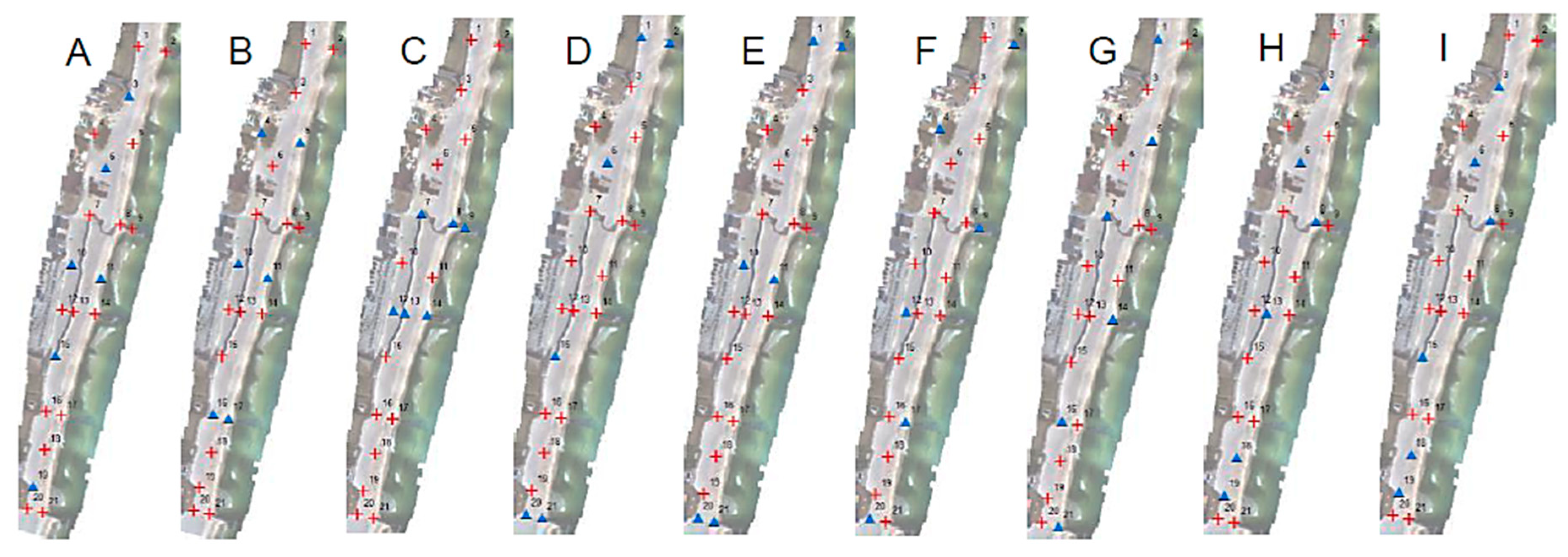
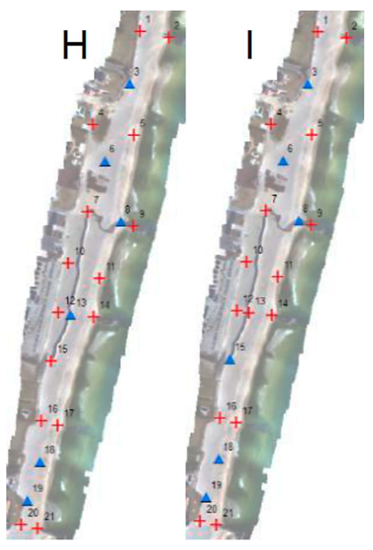
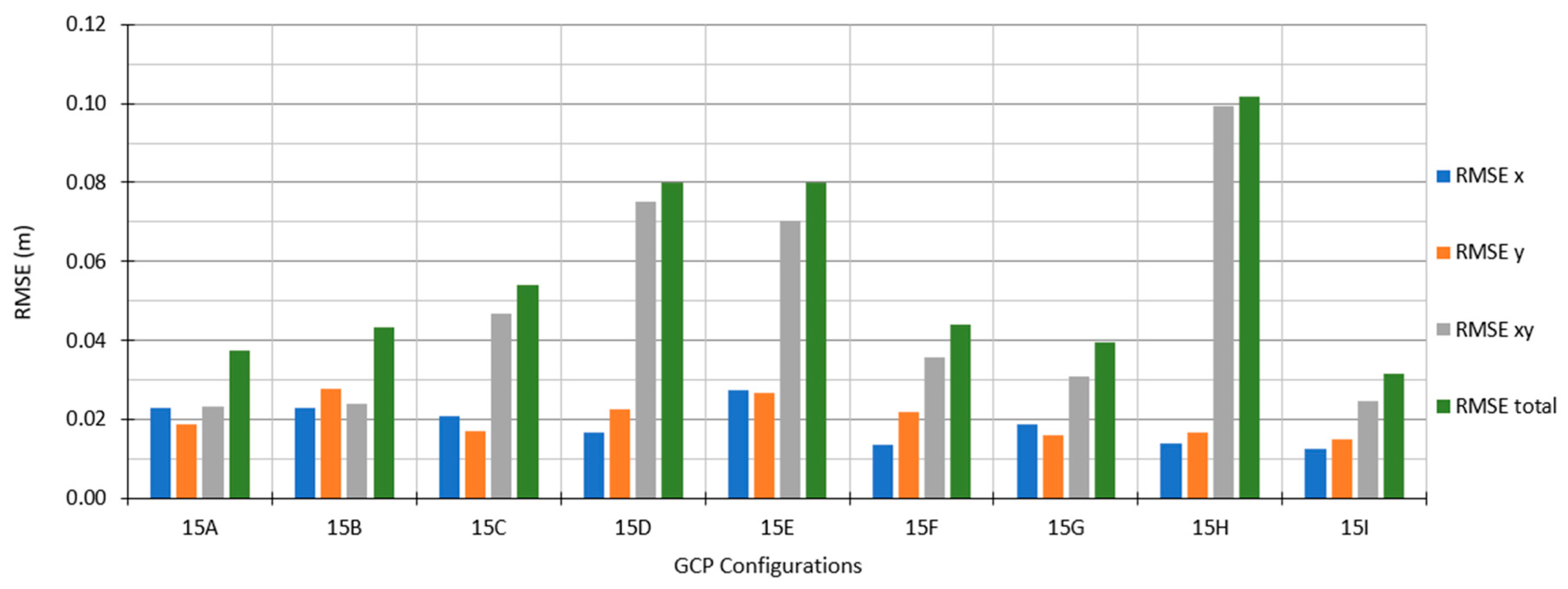
3.2.1. Configuration of Ground Control Points

To evaluate the sensitivity to configuration, or placement pattern, nine different variations of GCP configurations were analyzed using 15 GCPs and 6 check points. Figure 7 shows the nine variations (labeled A through I), where the GCPs are represented by a red plus sign (+) and the check points are represented by a blue triangle (). Figure 8 shows the corresponding horizontal, vertical, and total RMSE errors between the UAS-SfM generated DEM and the measured check points.
Maps D and E were the only variations that did not utilize GCPs in the four corners of the study area in georeferencing. Consequently, D and E show high vertical and total errors. The most significant pattern was observed between variations H and I, in which the former produced the greatest errors and the latter produced the smallest errors. Variations H and I are more clearly presented in Figure 9. The RMSEZ for variation H is 0.10 m (10 cm) and the RMSEZ for variation I is 0.03 m (3 cm). The only difference between the configurations of variation H and variation I are GCP 13 and GCP 15.
GCP 13 was used as a checkpoint in variation H (not used in georeferencing) and was used as a GCP (used in georeferencing) in variation I. The significance of including GCP 13 in georeferencing is that it is located on top of the winter berm, meaning it is the GCP with the highest elevation. This result is consistent with guidance that suggests that placing a GCP at the highest vertical elevation within the survey site is important in order to obtain high vertical accuracy [17]. Overall, the configuration of variation I resulted in the lowest errors. In variation I, the GCPs are placed in all four corners, have good cross-shore coverage, and include the highest site elevation. As a result of these findings, variation I was used as the basis for evaluating the influence of the amount of GCPs on accuracy.

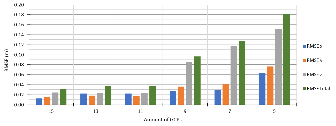
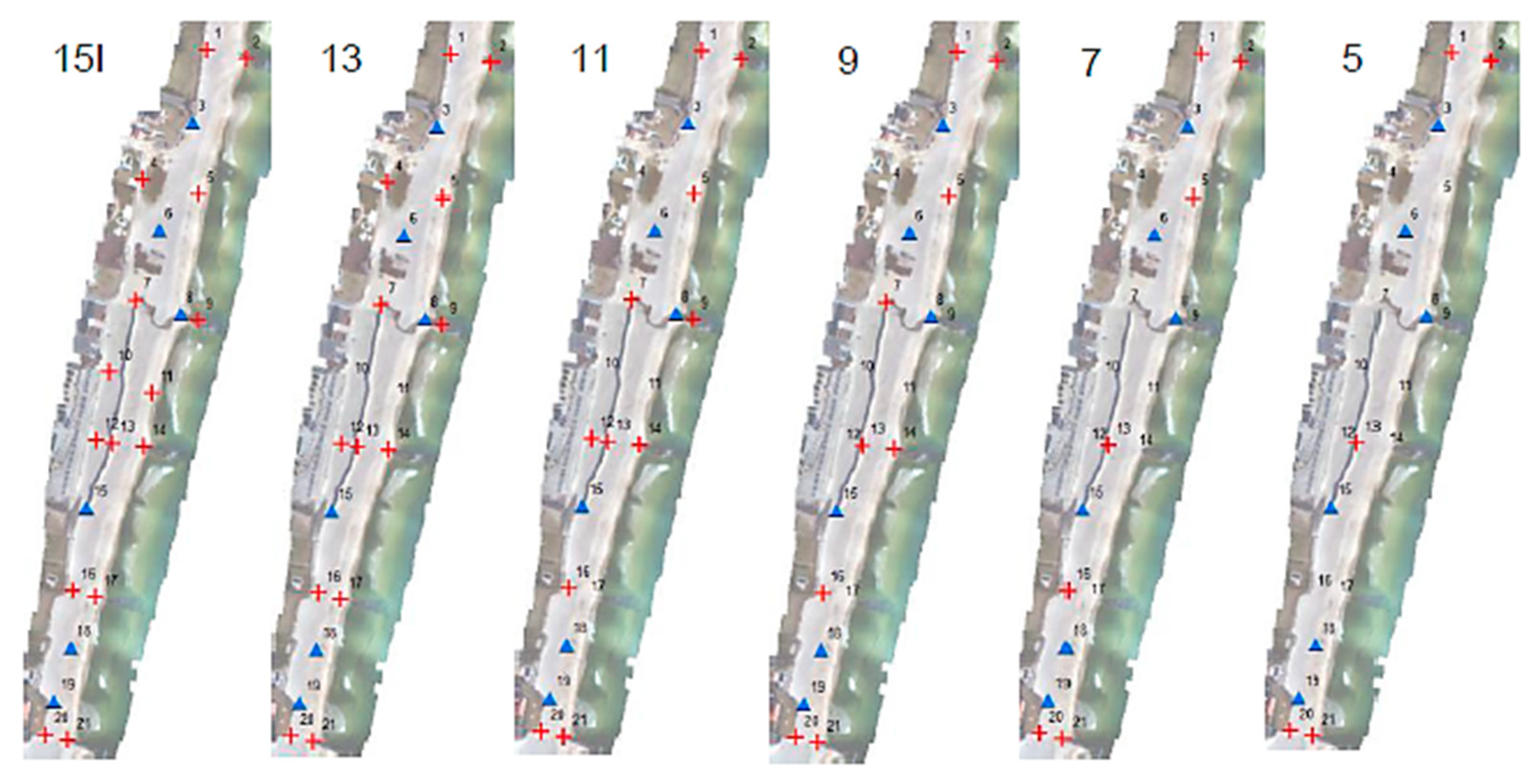
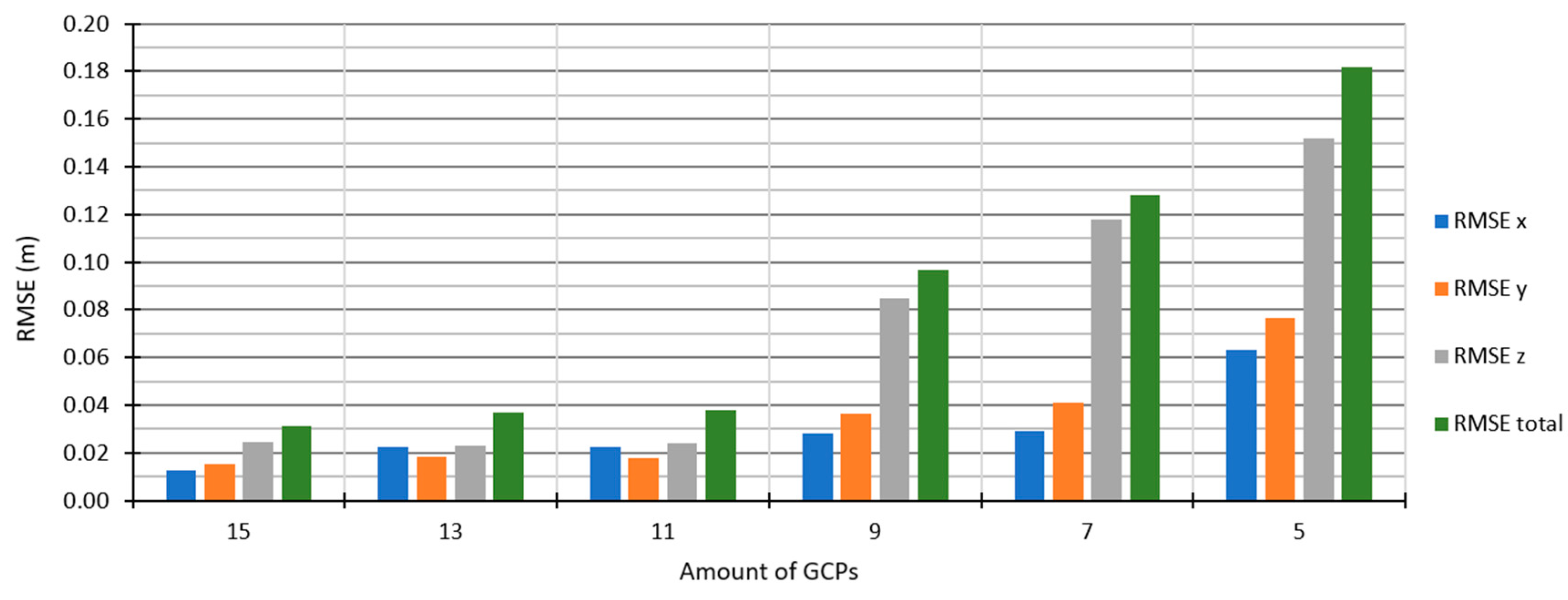
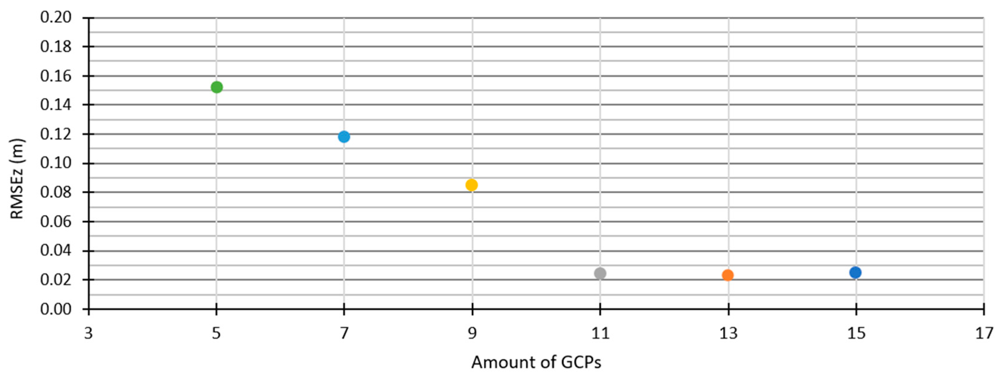
3.2.2. Amount of Ground Control Points

Utilizing the same GCP configuration as variation I, an analysis was performed that reduced the amount of GCPs used in georeferencing to understand the effect it has on the overall accuracy. Figure 10 shows the six different configurations of the reduced number of GCPs, starting with variation I (15 GCPs) and decreasing by two each time until only 5 GCPs are used. The maps are labeled according to the number of GCPs used in georeferencing. Figure 10 presents the GCP configuration maps, and Figure 11 shows the corresponding RMSE values.
The errors for 11, 13, and 15 GCPs are very similar with all RMSEZs at or below 0.03 m. When using 9 or less GCPs, the RMSEZs increase significantly. Under investigation of the configuration maps, this is likely a result of an insufficient amount of GCPs in the cross-shore. Specifically, both GCP number 9 (near shoreline) and GCP number 11 (near dune) were not used in georeferencing when using 9 GCPs or less.

4. Discussion

Monitoring beach morphology along developed coasts is extremely important, yet many traditional methods are insufficient in terms of spatial resolution, efficiency, or accuracy. The demonstrates the relevance of using UAS-SfM for beach surveying, as it mitigates most of the problems associated with traditional methods. Since UAS-SfM is often heavily dependent on proper ground control, a rigorous study such as this one is warranted to ensure the reliability and accuracy of the results.
An evaluation of UAS flight altitudes showed that the highest flight altitude tested, 116 m, was the most efficient in terms of survey time, processing time, and map accuracy. The check points from the 116 m flight yielded an average RMSEZ and RMSEtotal of 2.3 cm and 3.7 cm, respectively. For the lowest 67 m flight altitude, the RMSEZ was comparable at 3.7 cm, but the RMSEtotal was exceedingly large at 17.8 cm. These findings are consistent with recommendations provided by DroneDeploy for creating successful maps; by flying higher, the camera lens can cover more surface area per image [17]. When covering the maximum amount of surface area per single image, there are more chances to capture common unique features in multiple images. This is expected to be even more important at sites where many of the images are homogeneous. Flying higher provides the potential for more tie points to be recognized per image and therefore helps with mapping homogenous imagery, such as sandy beaches. Specific to the study site in Deal, the beach is highly developed such that there are residential homes that line the upland section of beach, which serve as fixed 3D structures with unique features that allow tie points to be more easily recognized.
The results of the investigation of GCP configurations and amounts demonstrated the magnitude of influence that the GCPs have on the accuracy of DEMs, and therefore the importance of using proper ground control. One of the most significant findings of GCP configuration was the importance of placing GCPs on the high and low areas of elevation. Colini et al. studied the application of remote sensing techniques, concentrating on photogrammetry and DEM generation, and found that placing GCPs at the high and low elevation points helped avoid planimetric and elevation extrapolations within the DEM [26]. This finding is consistent with the present work and is an important concept to understand and apply when setting up a survey and placing GCPs. This influence of GCP elevation was highlighted in Figure 9, which showed two GCP configurations that were the same aside from one pair of GCPs, where one was located at the highest elevation on the site. When the highest GCP was used in georeferencing, the total RMSE was approximately 3 cm, but when it was used as a check point (not used in georeferencing), the total RMSE was approximately 10 cm. Thus, the need to extrapolate the surface elevation resulted in a substantial increase in error and surface misrepresentation.
For the amount accuracy analysis, the amount of GCPs used in georeferencing varied from 5 to 15. It appeared that after 11 GCPs, the RMSEZ hit a plateau; this is displayed in Figure 12, which presents the relationship between the amount of GCPs and RMSEZ values. These data can be found in Figure 11, but they are presented here in a different/simpler way to better illustrate the relationship of interest.
There is a clear downward trend in RMSEZ from 5 to 9 GCPs, but a relatively unchanging RMSEZ for 11, 13, and 15 GCPs. Under further investigation of the configurations associated with the amount of GCPs, it is apparent that configurations with 11 or more GCPs provided sufficient cross-shore and alongshore coverage. Thus, it can be inferred that as long as there are GCPs in the four corners of the study site, in the highest and lowest elevations, and they have sufficient cross-shore coverage, the placement of GCPs is likely the predominant factor over the amount of GCPs. It is worth mentioning that advanced UAS with on-board RTK positioning receivers exist and can potentially reduce/eliminate the need for GCPs. However, it is possible that the optimal GCP configuration presented in this study could be applicable to surveys performed with RTK UAS. According to a report by Štroner et al., using a Global Navigation Satellite System (GNSS) RTK receiver in a UAS without external verification (such as GCPs) can be problematic, such that they can produce point clouds with relatively high systematic vertical errors [27]. This vertical shift in the entire point cloud is caused by caused by an incorrect identification of interior orientation parameters coupled with bundle adjustments. To rectify this problem, the authors recommended using a small amount of GCPs in the study area [27].

5. Conclusions

The study described in this paper was conducted to highlight and quantify the advantages of UAS to measure coastal morphology on a developed highly complex 3D beach, and specifically to find the optimal UAS and GCP parameters to produce the most accurate and efficient results. A section of the Deal, NJ coastline that contains a mix of old and newly modified structures that was the recipient of a recent beach nourishment was selected for this analysis. A sensitivity analysis was carried out to optimize UAS-SfM survey parameters including flight altitude, GCP configuration, and amount of GCPs. Three different flight altitudes were tested—67 m, 91 m, and 116 m. An altitude of 116 m was found to be the most efficient while also producing the most accurate results (nominally about 2 cm RMSE in the horizontal and vertical directions). Nine different GCP placement configurations were evaluated. The most accurate results, in terms of vertical and total RMSE (2.4 cm and 3.1 cm respectively), were found when GCPs were placed in (1) the four corners of the study area, (2) at the highest and lowest elevations, and (3) with sufficient cross-shore distribution. When the number of GCPs was varied within the optimal configuration, it was found that 15 GCPs produced the best results, but that as few as 11 GCPs could be used without any significant loss in accuracy. It was also observed that fewer (≈7–9) well-placed GCPs in the optimal configuration produced the same magnitude of error as using more (15) poorly placed GCPs. Based on the sensitivity analysis performed, the following recommendations are made for monitoring coastal morphology on highly complex 3D beaches:
  • The survey boundary should exceed the area of interest to ensure sufficient image overlap, guarantee GCPs are well-within survey area, and to account for potential influence of tidal range.
  • The highest flight altitude (116 m) resulted in the most accurate DEM (likely because each image covered the most surface area, allowing for more common features to be recognized in multiple images).
  • GCP configuration is critical, with optimal placement covering all four corners of the site, the highest and lowest elevations, and with sufficient cross-shore and alongshore coverage.
  • More GCPs do not always translate to better data; using less well-placed GCPs can yield more accurate results than using more poorly placed GCPs (likely related to spatial overfitting of the data) [25].
These recommendations reinforce the importance of project planning and survey setup as using fewer, strategically placed GCPs was more important and influential than using a greater amount of haphazardly placed GCPs. With that said, proper survey setup and ground control greatly influences the accuracy of the results; thus, it is crucial to consider the provided the guidelines when using UAS to measure coastal morphology.

Author Contributions

Conceptualization, J.M.; Data curation, K.J.; Formal analysis, T.Z.; Funding acquisition, J.M.; Investigation, T.Z. and K.J.; Methodology, K.J.; Project administration, J.M.; Resources, T.Z.; Software, T.Z.; Supervision, J.M.; Validation, T.Z.; Visualization, K.J and T.Z.; Writing—Original draft, T.Z.; Writing—Review and editing, J.M. All authors have read and agreed to the published version of the manuscript.

Funding

This research was funded by the New Jersey Department of Environmental Protection through the New Jersey Coastal Protection Technical Assistance Service under N.J.S.A 18A:64L-1.

Conflicts of Interest

The authors declare no conflict of interest. The funders had no role in the design of the study; in the collection, analyses, or interpretation of data; in the writing of the manuscript, or in the decision to publish the results.

References

  1. Theuerkauf, E.J.; Rodriguez, A.B. Impacts of Transect Location and Variations in Along-Beach Morphology on Measuring Volume Change. J. Coast. Res. 2012, 28, 707–718. [Google Scholar]
  2. Mason, D.; Gurney, C.; Kennett, M. Beach Topography Mapping—A Comparison of Techniques. J. Coast. Conserv. 2000, 6, 113–124. [Google Scholar] [CrossRef]
  3. Lee, J.M.; Park, J.Y.; Choi, J.Y. Evaluation of Sub-aerial Topographic Surveying Techniques Using Total Station and RTK-GPS for Applications in Macrotidal Sand Beach Environment. J. Coast. Res. 2013, 65, 535–540. [Google Scholar] [CrossRef]
  4. Terefenko, P.; Wziatek, D.Z.; Dalyot, S.; Boski, T.; Lima-Filho, F.P. A High-Precision LiDAR-Based Method for Surveying and Classifying Coastal Notches. ISPRS Int. J. Geo-Inf. 2018, 7, 295. [Google Scholar] [CrossRef] [Green Version]
  5. Spore, N.J.; Renaud, A.D.; Conery, I.W.; Brodie, K.L. Coastal Lidar and Radar Imaging System (CLARIS) Lidar Data Report: 2011–2017; ERDC/CHL SR-19-4; Engineer Research and Development Center Vicksburg Ms Vicksburg: Vicksburg, MS, USA, 2019; pp. 4–7. [Google Scholar]
  6. Papakonstantinou, A.; Topouzelis, K.; Pavlogeorgatos, G. Coastline Zone Identification and 3D Coastal Mapping Using UAV Spatial Data. ISPRS Int. J. Geo-Inf. 2016, 5, 75. [Google Scholar] [CrossRef] [Green Version]
  7. Jansen, M.K. Analysis of Photogrammetric Mapping Using Low-Cost Unmanned Aerial Vehicles in Coastal Areas. Master’ Thesis, Stevens Institute of Technology, Hoboken, NJ, USA, 2 May 2018. [Google Scholar]
  8. Spore, N.J.; Brodie, K.L. Collection, Processing, and Accuracy of Mobile Terrestrial Lidar Survey Data in the Coastal Environment; ERDC/CHLH TR-17-5; Field Research Facility, US Army Engineer Research and Development Center: Kitty Hawk, NC, USA, 2018; pp. 1–29. [Google Scholar]
  9. Basco, D.R.; Pope, J. Groin Functional Design Guidance from the Coastal Engineering Manual. J. Coast. Res. 2004, 33, 121–130. [Google Scholar]
  10. FACT SHEET—Sea Bright to Manasquan, NJ Coastal Storm Risk Management and Erosion Control Project. Available online: https://www.nan.usace.army.mil/Media/Fact-Sheets/Fact-Sheet-Article-View/Article/487661/sea-bright-to-manasquan-nj-beach/ (accessed on 5 March 2020).
  11. Sandy Hook to Barnegat Inlet, NJ. Available online: https://www.nan.usace.army.mil/Missions/Civil-Works/Projects-in-New-Jersey/Sandy-Hook-to-Barnegat-Inlet/ (accessed on 5 July 2020).
  12. Phantom 4 Specs. Available online: https://www.dji.com/phantom-4 (accessed on 5 March 2020).
  13. Commercial Operations Branch Part 107 UAS Operations. Available online: https://www.faa.gov/about/office_org/headquarters_offices/avs/offices/afx/afs/afs800/afs820/part107_oper/ (accessed on 5 March 2020).
  14. Structure from Motion Introductory Guide. Available online: https://www.unavco.org/education/resources/modules-and-activities/field-geodesy/module-materials/sfm-intro-guide.pdf (accessed on 1 March 2020).
  15. James, M.; Robson, S.; Smith, M. 3-D uncertainty-based topographic change detection with structure-from-motion photogrammetry: Precision maps for ground control and directly georeferenced surveys. Earth Surf. Process. Landf. 2017, 42, 1769–1788. [Google Scholar] [CrossRef]
  16. Georeferencing. Available online: https://serc.carleton.edu/research_education/geopad/georeferencing.html (accessed on 29 April 2020).
  17. Ground Control Points. Available online: https://support.dronedeploy.com/docs/working-gcp-step-by-step (accessed on 29 April 2020).
  18. Agisoft Metashape User Manual. Available online: https://www.agisoft.com/pdf/metashape-pro_1_5_en.pdf (accessed on 25 April 2020).
  19. Tahar, K.N. An Evaluation on Different Number of Ground Control Points in Unmanned Aerial Vehicle Photogrammetric Block. Int. Arch. Photogramm. Remote Sens. Spat. Inf. Sci. 2013, XL-2/W2, 93–98. [Google Scholar] [CrossRef] [Green Version]
  20. Brunier, G.; Fleury, J.; Anthony, E.J.; Gardel, A.; Dussouillez, P. Close-range airborne Structure-from-Motion Photogrammetry for high-resolution beach morphometric surveys: Examples from an embayed rotating beach. Geomorphology 2016, 261, 76–88. [Google Scholar] [CrossRef]
  21. Seifert, E.; Seifert, S.; Vogt, H.; Drew, D.; Aardt, J.; Kunneke, A.; Seifert, T. Influence of Drone Altitude, Image Overlap, and Optical Sensor Resolution on Multi-View Reconstruction of Forest Images. Remote Sens. 2019, 11, 1252. [Google Scholar] [CrossRef] [Green Version]
  22. Pix4D Documentation Ground Sampling Distance. Available online: https://support.pix4d.com/hc/en-us/articles/202559809-Ground-sampling-distance-GSD (accessed on 5 March 2020).
  23. Pix4D Documentation Difference between a Ground Control Point and a Check Point. Available online: https://support.pix4d.com/hc/en-us/articles/115000140963-Difference-between-a-ground-control-point-and-a-checkpoint (accessed on 5 March 2020).
  24. Jayaratne, M.P.; Rahman, M.; Shibayama, T. A Cross-Shore Beach Profile Evaluation Model. Coast. Eng. J. 2015, 56, 40. [Google Scholar]
  25. Rizeei, H.M.; Pradhan, B. Urban Mapping Accuracy Enhancement in High-Rise Built-Up Areas Deployed by 3D-Orthorectification Correction from WorldView-3 and LiDAR Imageries. Remote Sens. 2019, 11, 692. [Google Scholar] [CrossRef] [Green Version]
  26. Colini, L.; Doumaz, F.; Buongiorno, M.F.; Neri, M.; Mazzarini, F. Generation of high resolution Digital Elevation Models using Remote Sensing optical stereo data: Application to Mount Etna test site, Italy. In Geophysical Research Abstracts, Proceedings of the European Geosciences Union, Vienna, Austria, 2–7 April 2006; European Geosciences Union: Munich, Germany, 2006; Volume 8, p. 07583. [Google Scholar]
  27. Štroner, M.; Urban, R.; Reindl, T.; Seidl, J.; Brouček, J. Evaluation of the Georeferencing Accuracy of a Photogrammetric Model Using a Quadrocopter with Onboard GNSS RTK. Sensors 2020, 20, 2318. [Google Scholar] [CrossRef] [PubMed] [Green Version]
Figure 1. Surveyor equipped with a real-time kinematic global positioning system (RTK GPS) backpack taking measurements up a sloped beach.
Remotesensing 12 02305 g001
Figure 2. Site Location Map—Deal, New Jersey, USA.
Remotesensing 12 02305 g002
Figure 3. Unmanned Aerial Systems (UAS) aerial images of: (a) Notched groin at Deal beach with a box depicting the notch area or the section of groin removed; (b) Typical traditional groin at Deal beach.
Remotesensing 12 02305 g003
Figure 4. Example flight planning input in DroneDeploy Software.
Remotesensing 12 02305 g004
Figure 5. Examples of ground control points (a) Surveying the ground control point (GCP) position using an RTK GPS spot measurement system; (b) A typical view of a GCP from an UAS aerial image.
Remotesensing 12 02305 g005
Figure 6. Check point RMSEs for various UAS flight altitudes.
Remotesensing 12 02305 g006
Figure 7. Variations of GCP configurations (GCPs (+) and check points (▲)).
Remotesensing 12 02305 g007
Figure 8. Check point RMSEs of the variations of GCP configurations.
Remotesensing 12 02305 g008
Figure 9. GCP Configurations for variation H and variation I (GCPs (+) and check points (▲)).
Remotesensing 12 02305 g009
Figure 10. Configurations of the different amounts of GCPs tested on variation I (GCPs (+) and check points (▲)).
Remotesensing 12 02305 g010
Figure 11. Check point RMSEs of the different amounts of GCPs tested on variation I.
Remotesensing 12 02305 g011
Figure 12. Relationship between the amount of GCPs and RMSEz.
Remotesensing 12 02305 g012
Table 1. Comparison of Surveying Systems and Associated Characteristics [3,7,8]. LiDAR: light detection and ranging.
Data Collection SystemCostTime of SurveyPoint Density (points/m3)Accuracy (meters)
Quadcopter UAS$1000Low≃50–100≃0.03
RTK GPS Backpack$15,000High≃1–2≃0.05
RTK GPS Spot Measurement$15,000Very high≃0.20–1≃0.02
Terrestrial LiDAR$50,000High≃100–1000≃0.012
Airborne LiDAR$100,000High≃1–10≃0.15
Table 2. UAS Survey Flight Altitude Parameters.
Flight Altitude (m)Flight Duration (hh:mm:ss)Batteries UsedTotal Number of ImagesGround Sampling Distance (GSD) (cm)Agisoft Photoscan Processing Time (hh:mm:ss)
6700:54:0038711.678:40:01
9100:38:0024862.274:47:07
11600:28:0013172.893:00:23
Table 3. UAS survey flight altitude accuracy assessment with RTK GPS walker data. RMSE: root mean square error.
Flight Altitude (m)Amount of GCPsBias (m)Standard Deviation (m)RMSEZ (m)
6721−0.1290.05490.140
15−0.1240.05760.137
9121−0.1300.05120.139
15−0.1270.05490.139
11621−0.1380.04970.147
15−0.1340.05090.143

