Abstract
The Karakoram has had an overall slight positive glacier mass balance since the end of 20th century, which is anomalous given that most other regions in High Mountain Asia have had negative changes. A large number of advancing, retreating, and surging glaciers are heterogeneously mixed in the Karakoram increasing the difficulties and inaccuracies to identify glacier surges. We found two adjacent glaciers in the eastern Karakoram behaving differently from 1995 to 2019: one was surging and the other was advancing. In order to figure out the differences existing between them and the potential controls on surges in this region, we collected satellite images from Landsat series, ASTER, and Google Earth, along with two sets of digital elevation model. Utilizing visual interpretation, feature tracking of optical images, and differencing between digital elevation models, three major differences were observed: (1) the evolution profiles of the terminus positions occupied different change patterns; (2) the surging glacier experienced a dramatic fluctuation in the surface velocities during and after the event, while the advancing glacier flowed in a stable mode; and (3) surface elevation of the surging glacier decreased in the reservoir and increased in the receiving zone. However, the advancing glacier only had an obvious elevation increase over its terminus part. These differences can be regarded as standards for surge identification in mountain ranges. After combining the differences with regional meteorological conditions, we suggested that changes of thermal and hydrological conditions could play a role in the surge occurrence, in addition, geomorphological characteristics and increasing warming climate might also be part of it. This research strongly contributes to the literatures of glacial motion and glacier mass change in the eastern Karakoram through remote sensing.
1. Introduction
As a key indicator of climate variability, changes in mountain glaciers contribute to sea-level rise and sometimes induce flood hazards to local and downstream residences [1,2,3,4]. Although only a small number, less than 1%, of these mountain glaciers are surge-type glaciers [5], they play an important role in the research of flow instabilities and modern glacier processes [6,7]. Most surge-type glaciers undergo active phases and quiescent phases occurring in a way of quasiperiodic oscillation [8,9]. During the active phases, the flow velocities increase dramatically by 10–100 times over a span of months to years, accompanied by terminus advancing in most cases [6,10]. Meanwhile, a large volume of ice is discharged from the reservoir zones in the upstream to the receiving zones in the downstream [9,11]. During the quiescent phases lasting years to decades, new ice is recharged in the reservoirs and the discharged ice in the receiving zones recedes progressively [9,11]. Some glacier surges could also lead to debris flows and glacial lake outburst floods. Therefore, a rising number of literatures have been published focusing on their evolution and distribution [7,12,13,14].
Rather than external forcing, it is generally recognized that surges are generated by the alteration of internal conditions within and beneath ice mass [8,15,16]. Among various models interpreting surging mechanisms, the models of hydrologically controlled surges and thermally controlled surges are two well-accepted ones, which are also, respectively, referred to the “Alaska” type and the “Svalbard” type [17,18,19,20]. Hydrologically controlled surges are usually initiated by the changes in hydrological system and pore water pressure [18,21]. They are suggested to initiate in winter when the drainage system is inefficient and terminate in summer when melting water reduces inner water pressure [10]. The initiation and termination phases of hydrologically controlled surges are very short, lasting days to weeks [20,22,23]. In this model, the surge front locates the boundary between the inefficient cavitized drainage system in the downstream and the efficient tunnel drainage system in the upstream [24]. Thermally controlled surges are caused by the increasing basal temperature resulting in sediment deformation and increase in pore water pressure [17,25]. These surges have no obvious seasonal control on their initiations and terminations, but are characterized by relatively long durations (several years) before and after the peak of surges [25]. The surge fronts represent the transition zones between warm-based ice mass in the up-glacier direction and the cold-based ice mass in the down-glacier direction [26]. Besides, some reports in the Karakoram and the Pamir considered that distinctive glacial morphology could have a relationship with the formation of surge fronts [22,27].
The earliest scientific reports about glacier surges were from researches in the Alaska and the Svalbard [9,28]. Since then, this endmember of glacier flow has been documented all around the world, especially in polar regions and North America [29,30,31]. It is until the recent decade that an increasing attention has been paid to glacier surges in the Karakoram [15,22,32,33,34,35]. Karakoram is not only being regarded as an optimal surge zone [7] but is also anomalous for its positive glacier mass budget since the end of 20th century during which time glaciers in other regions on Earth have been continuously losing ice [36,37,38]. Although debate still exists on whether climate warming has a favorable contribution to occurrences of glacier surges in the Karakoram, there are indications suggesting that surge frequency might have increased since 1990 [15,34,39,40]. As ice mass gain can contribute to speed up of glacier flow, and thus lead to terminus advance, large number of advancing glaciers and surge-type glaciers are heterogeneously mixed in this region [34,41]. It raises difficulty and reduces accuracy for surge identification in the Karakoram. Although previous research suggested that surges in the Karakoram are triggered by a blend of hydrological and thermal processes [22], the mechanism of surge initiation and clustering in the Karakoram and surrounding regions, such as the Pamir and the Kunlun Shan, is far from completely known [27,34,36,42,43].
Due to the harsh environment and remoteness of glaciers in the Karakoram, in-situ glaciological studies are time consuming and hard to carry out [15,35]. Development of remote-sensing technology makes it possible to exhaustively evaluate temporal and spatial changes of glaciers [44,45]. Utilizing abundant satellite images in the existing global archive, researchers are able to extract glacial boundaries and glacial surface displacements between different years [46,47,48]. In addition to this, a growing number of digital elevation models (DEMs) covering glacierized area are released each year [49]. By coregistering DEMs acquired at separate time, glacier thickness change during certain period can be quantified, which has a close connection with regional glacier mass balance [50].
We found two adjacent glaciers in the eastern Karakoram behaving differently since 1990s: a surging one and an advancing one. The objective of this paper is to compare the differences between these two glaciers in horizontal and vertical directions through remote sensing. In doing this, we provide a remote-sensing standard for surge identification in this region. Supported by analysis of glacial hypsometry and records from surrounding meteorological stations, we give our reasons on the glacial flow heterogeneity and discuss possible controls on surge mechanism in the Karakoram.
2. Study Area
The eastern Karakoram is part of High Mountain Asia and mostly lies in the southwest of Xinjiang, China (Figure 1). The eastern Karakoram has a glacierized area of 5988 km2, which contributes 11.6% to the total glacier area in China [51]. These glaciers share termini elevations of 4200–4700 m a.s.l. and equilibrium line altitudes of 5100–5400 m a.s.l. [52,53]. The glacial melt water feeds directly to the Yarkand and the Indus rivers and thus plays a vital role in supporting agriculture and livestock for nearly 130 million people in the downstream [54,55]. Shaksgam River flows through the valley in the eastern Karakoram (Figure 1). Mount Chhogori, also known as the name of “K2”, and Gasherbrum I stand to the south of the valley, and to the north side is the Aghil Mountains [56]. Our two studied glaciers are located in the Aghil Mountains stretching in a northwest to southeast direction. The surging glacier is given symbol “S” and the advancing one is given symbol “A” (Figure 1). They occupy almost the same aspects (Table 1) and are both recorded in the Randolph Glacier Inventory (RGI) [29]. Compared to some heavily debris-covered glaciers with long glacier tongues in the Karakoram, the tongues of these two glaciers have relatively cleaner surfaces.
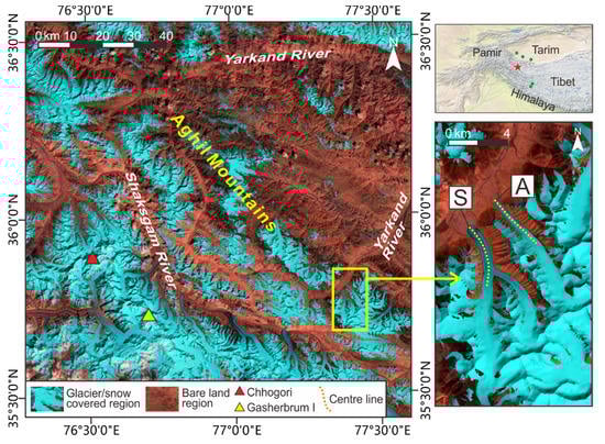
Figure 1.
Landsat 8 OLI image (band combination of 6, 5, and 4) of the study area on 8 September 2016. The red star in the topographic map locates the studied glaciers and the green spots represent the locations of meteorological stations in Figure 7.

Table 1.
Attributes of the two studied glaciers. Glacier areas are detected based on the images of 17 August 1999 and 3 October 2019. Longitude and latitude represent the central position of the glaciers. Zmed represents median elevation and SLA represents snowline altitude in 2019.
Climate in the eastern Karakoram is impacted by both Asian monsoon and high-altitude westerly circulation [39]. During summer, the precipitation is predominantly caused by Asian monsoon, while the winter precipitation is contributed mostly by westerly circulation, especially in the high-altitude regions [39]. The average precipitation reported in the Karakoram can reach 1174 mm a−1 at 6000 m a.s.l. [57]. An increasing trend in precipitation leads to a positive water equivalent (w.e.) mass balance of 0.10 ± 0.16 m w.e. a−1 during the period of 1999–2010 [39,58,59].
3. Data
3.1. Satellite Imagery
We totally utilized 6 Landsat 5 Thematic Mapper (TM), 14 Landsat 7 Enhanced Thematic Mapper Plus (ETM+), 8 Landsat 8 Operational Land Imager (OLI), and 2 ASTER L1T images with minimal snow and cloud cover from 1995 to 2019 (Supplementary Table S1). Most images were used to detect the sequential evolution of glacial terminus. By feature tracking, we conducted Landsat 5 and Landsat 7 images before 2003 and Landsat 8 images after 2013 to extract glacial surface displacements. Considering the failure on the Landsat 7 hardware in May 2003, we tried to use ASTER and Landsat 5 images to do feature-tracking work between 2003 and 2013 and fortunately generated two good cross-correlation results (2006–2008 and 2008–2011) (Table S1). Most images used for displacement extraction have a spatial resolution of 15 m (i.e., panchromatic bands of Landsat 7 and Landsat 8 and band 3N of ASTER), except for band 4 of Landsat 5 with 30 m spatial resolution leading to relatively coarser results. We selected each image pair containing two images from the same sensor. Therefore, no further radiometric and geometric corrections are needed before feature tracking [27]. All these images were acquired from the USGS Earth Resources Observation and Science Center (EROS) (http://glovis.usgs.gov, last access: 30 April 2020). We also used a high-spatial-resolution image from Google Earth (data provided by Maxar Technologies) to interpret distinct surface features.
3.2. DEM
We used two different sets of DEM in this study. One is Shuttle Radar Topography Mission (SRTM) DEM. This near-global dataset was generated from data of a C-band radar during the period of 11–22 February 2000. We downloaded nonvoid-filled SRTM DEM (version 1.0) and void-filled SRTM DEM (version 3.0) covering the region of 35–36° N and 077–078° E from USGS EarthExplorer (https://earthexplorer.usgs.gov, last access: 30 April 2020). The void-filled SRTM DEM has a better resolution of 1 arc-second than the nonvoid-filled SRTM DEM with a 3 arc-second resolution. The void-filled SRTM also has a better accuracy of less than 10 m in horizontal and vertical directions [60]. However, elevation data used for filling voids does not have an extract time, which could increase uncertainty in calculating glacier mass changes. Luckily, we found that the voids in the unfilled SRTM DEM mainly affect some steep mountain slopes nearby and both of our studied glaciers are covered entirely by the nonvoid-filled SRTM DEM. Therefore, we chose the void-filled tile as the reference elevation data during DEM coregistration, because it represents the true condition of the glacier surface in February 2000 with a higher spatial resolution. The other one is High Mountain Asia 8-meter DEM (HMA DEM) released by NASA National Snow and Ice Data Center in 2017 [49]. The tile we used in this study was generated from an along-track stereoscopic image pair acquired ~60 s apart on 10 November 2015 by DigitalGlobe satellites (Table S1). It was downloaded from NASA Earthdata (https://earthdata.nasa.gov, last access: 30 April 2020). Before coregistration with each other, both DEMs were resampled to 30 m spatial resolution and projected to the same coordinate system. The DEMs were used to calculate ice volume change, along with topographic and hypsometric analysis in support of surge mechanism discussion.
3.3. Glacier Inventory and Meteorological Data
We chose RGI version 6.0 as baseline for glacier delineation and manually modified boundaries for two studied glaciers in years 1999 and 2019. RGI data was acquired from Global Land Ice Measurements from Space (GLIMS) (https://glims.org, last access: 30 April 2020). It was mainly used for glacier delineation and glacierized region deduction from the DEMs during the process of coregistration.
We identified the locations of surrounding meteorological stations and acquired their temperature records from the Global Historical Climatology Network-monthly (GHCNm) version 4. GHCNm is a dataset of monthly climate records from weather stations around the world [61]. It was downloaded from National Oceanic and Atmospheric Administration (NOAA) (http://ncdc.noaa.gov, last access: 30 April 2020).
4. Methods
4.1. Glacier Delineation
With the help of RGI and high-spatial-resolution images from Google Earth, we manually delineated outlines for the two glaciers in 1999 and 2019 based on features in Landsat images (Table S1). We also digitized glacial terminus changes along their center lines from 1995 to 2019. Manual delineation of glacier termini and outlines would nevertheless not get consistent results [62]. Applying the method suggested by previous study, we repeatedly delineated two studied glaciers in the same image for five times (at least two hours apart for each time) and chose their standard deviations as the accuracies of manual delineation [63]. The final accuracy of glacial area measurement is 1.97%, and the accuracy of glacial terminus measurement is 6.49 m.
4.2. Detection of Glacial Motion
We extracted displacements on glacier surface by conducting coregistration and correlation to optical images using a feature-tracking software called Co-registration of Optically Sensed Images and Correlation (COSI-Corr) [64]. Research has proved that this software package is effective in quantifying glacier surface displacement from optical imagery [27]. Image pairs were firstly coregistered in the same reference system. By using a sliding window pixel by pixel across the image with a frequential subpixel correlator, horizontal displacements then could be measured along the north-south and east-west directions separately. We changed the sliding window size from 32 32 to 8 8, following the recommendation of previous study [27]. Total displacements were obtained after combining displacements in north-south and east-west directions. Glacier velocity () can be calculated through Equation (1).
where D represents the measured displacement in meters, is given the number of 365 presenting days in a year, and is the interval period (days) between the acquisition time of the images. Thus, the unit of is meters per year (m a−1). To compare the interannual changes for the studied glaciers, velocity profiles in different years were extracted along their center lines and put together.
Decorrelation is unavoidable during glacial motion detection in mountain regions, due to the limitation of clear surface feature in optical satellite images. To reduce such impact, we smoothed the displacement map using a Gaussian low-path filter with a kernel size of 3 3. We also manually removed blunders, which differed by >20 m a−1 comparing to neighboring areas (within 5 pixels).
Considering off-glacier areas should scarcely experience any horizontal changes under natural conditions, we suggested that the residual value in stable (off-glacier) terrain could reflect the error of displacement extraction. As the velocity results were generated from images with two different spatial resolutions, the errors from Landsat 5 TM and other sensors were calculated separately. Statistically, the uncertainty was 3.74 m a−1 for Landsat 5 results and 0.96 m a−1 for the other sources. It shows that the feature-tracking result is precise enough to present glacial motion changes in this region.
4.3. Calculation of Glacier Mass Change
In areas of ice and snow, penetration of C-band radar signal, which is used to generate SRTM DEM, can be problematic [65]. Therefore, SRTM DEM should be modified before coregistration with HMA DEM. One Landsat 7 image around the acquisition time of SRTM (February 2000) was classified to identify different ice and snow facies. We applied a threshold of 2.2 to TM3/TM5 band ratio of Landsat 7 to extract ice- and snow-covered regions. Snow-covered region was separated from clean ice by applying a threshold of 200 after stretching (TM4 × TM2)/TM5 to the range of 0 to 255 [66]. Following the results of previous study in the Karakoram, we conducted a correction of +5.5 m to snow-covered region and +1.1 m over clean ice [66]. Some part of Glacier S was covered by debris (Figure 1) and it could be seen in the Landsat 7 image in February 2000 clearly. The radar signal could hardly penetrate rock surface, and we thus retained the SRTM elevation data over debris-covered area unchanged.
Because of sensor instabilities and different post-processing procedures, inconsistent biases might exist between SRTM DEM and HMA DEM [50]. Before calculating glacier mass changes, we coregistered the HMA DEM to the SRTM DEM based on a three-step coregistration process proposed by Nuth and Kääb [50]. At first, mismatches were identified and removed through turning and shifting the HMA DEM on the basis of slope and aspect differences between the DEMs. Then, a linear relationship between elevations and differences was applied to adjust elevation-dependent biases. Thirdly, higher-order biases resulting from satellite geometry were checked and corrected.
After coregistering HMA DEM and SRTM DEM, we found that there were still registration errors existing in the map of elevation differences. Given that vertical elevations should not change obviously over stable terrain from 2000 to 2015, we discarded changes greater than 3 standard deviations over off-glacier region [67]. The mean difference over off-glacier area is 0.89 m and the standard deviation () is 8.03 m, which is an essential element for error assessment in the following section. We also discovered some outliers locating at high-elevation zones and steep slopes as a possible result of poor feature matching during photogrammetric generation of HMA DEM. To deal with these outliers, we adjusted a threshold of ±48 m to areas above glacial median elevation. After visual interpretation, no clear ice avalanche was detected on both glaciers during study period. Thus, we assumed the elevation changes in this part could not continuously exceed 3 m a−1 from 2000 to 2015.
In order to calculate glacier-wide mass balance, we filled the data gaps over the studied glaciers. For gaps less than 5 5 grid cells, the filling values were taken from the mean changes of surrounding pixels. For other large gaps, we filled them using the mean differences at the corresponding elevation level by cutting the difference map into several 100 m elevation bands [67]. This was achieved in the software of ArcGIS 10.6. After filling all gaps, ice volume change of each glacier () was summed by volume change in every pixel (Equation (2)).
where represents the elevation change of every pixel and represents the pixel area in the DEM, which is 900 m2 in our study. Total glacier mass change () is calculated through Equation (3).
where is the glacier density for converting ice mass to water equivalent mass. In this study, is given the value of 850 kg m−3 with an uncertainty () of 60 kg m−3 [68]. A is the area of each glacier and is the number of years between the SRTM DEM and the HMA DEM. The unit of is m w.e. a−1.
4.4. Error Assessment of Glacier Mass Change
The uncertainty in glacier mass change is mainly resulted from the elevation change error, the area measurement uncertainty, and the density conversion uncertainty [69]. Assuming seasonal change over one decade in our study area to be negligible, we applied no seasonal correction to the final mass change uncertainty.
As two studied glaciers both have large enough areas, errors in elevation changes () were defined through Equation (4) suggested by previous research [70].
where is the standard deviation of elevation change over off-glacier terrain, is the area of each glacier, and is the spatially correlated area which is calculated by Equation (5).
We gave a value of 400 m to the decorrelation length () between HMA DEM and SRTM DEM [71]. It should be noted that would not be the same for other DEMs with different original spatial resolutions.
The final error of the annual mass change () was estimated by Equation (6.)
where is the factor of density conversion given 0.85 and its uncertainty () is given 0.06. The area measurement uncertainty () discussed in Section 4.1 is 1.97% for both glaciers. As data voids may have an impact on the error assessment, available data-cover rate () is also taken into the final consideration [72].
5. Results
The surging glacier (Glacier S) has two major tributaries in its upstream with a broader glacier tongue than the advancing glacier (Glacier A) (Figure 1). They both have an aspect facing north direction and have advanced in the same direction since the 21st century. The slope of Glacier S is slightly lower than that of Glacier A. In 2019, the area proportions above SLA for Glacier S and Glacier A are 72.6% and 90.9%, respectively. From 1999 to 2019, the increased area of Glacier S was 0.95 km2 which is larger than the 0.18 km2 of Glacier A (Table 1). However, compared to the individual areas in 1999, Glacier S increased an area of 3% and Glacier A increased 1%. The area change ratios are not significantly different to tell apart surging and advancing processes.
5.1. Visual Interpretation
Evolution of Glacier S and Glacier A is shown in Figure 2. Glacier A had a clean and smooth glacier tongue, whereas deformed debris-cover feature and heavy surface crevassing could clearly be seen on Glacier S from Google Earth image in 2010. The terminus shape of Glacier A remained almost the same from 1996 to 2019. Judging from Landsat images, Glacier S was in a shrinkage stage in 1996. In 2000, the tongue of Glacier S was already broadened by the surge. After 2000, the debris cover on Glacier S deformed obviously along with an advance of its terminus. Till 2019, its terminus shape had changed and moved to the downstream valley. Remnant of looped moraine still existed on the terminus part of Glacier S in 2019.
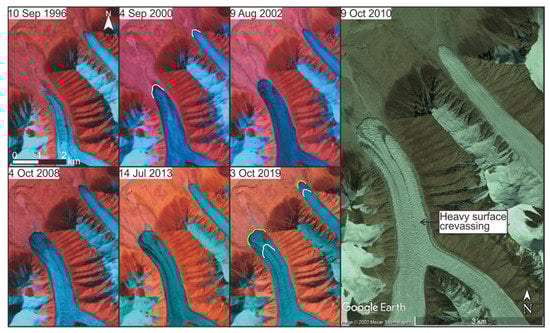
Figure 2.
Satellite images of the two studied glaciers at different time. Six images on the left are false-color combination of Landsat series and the big image on the right is from Google Earth. The white and yellow lines, respectively, indicate the terminus positions in 2000 and 2019.
We manually measured the changes of glacier terminus positions and plotted them together (Figure 3). From 1995 to 2019, the terminus of Glacier A advanced 444.25 m and of Glacier S advanced 971.36 m, nearly twice of Glacier A. The differences lay not only in the value of final distances but also in the shape of terminus evolution curves. Glacier A had a linear terminus evolution curve with a slope of ~20 m a−1 during the studied period. It showed no sign of deceleration suggesting that Glacier A might keep advancing in the next few years in the same velocity. For the terminus of Glacier S, an abrupt change occurred in 1999 and this rapid advance did not slow down until 2001. Not until 2017 did its terminus stabilize. Judging by previous studies on glacier surges in the eastern Pamir, we suggested that the terminus of Glacier S would not move forward in the near future, but experience a retreat instead [27].
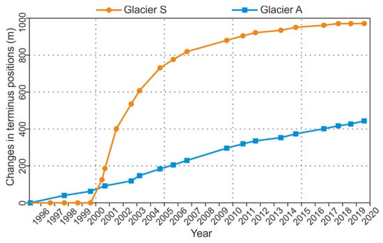
Figure 3.
Evolution of glacier terminus positions from 1995 to 2019.
5.2. Glacier Velocity Change
In order to figure out more details in glacial surface discrepancy between a surge event and a normal advance, annual surface velocity profiles of Glacier S and Glacier A were extracted separately (Figure 4). The most obvious difference is the magnitude order velocity variation on Glacier S, while Glacier A was consistent within a narrow range.
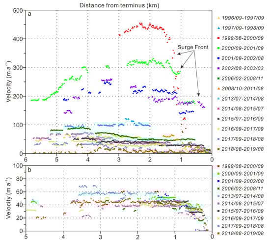
Figure 4.
Centre line annual-velocity profiles for the studied glaciers: (a) Glacier S and (b) Glacier A. Note that velocity profiles extracted from Landsat 5 images are presented using small triangles in (a). Zero point on x-axis is terminus at maximum extent.
Telling from Figure 4a, Glacier S was in its quiescent phase in 1996 and flowed in a velocity of 40–50 m a−1. Its surface velocity started accelerating from 1997 when the active phase of the surge began. Two years later, in 1999, its surface velocity achieved the peak (450 m a−1), which was almost 9–10 times of its velocity before the surge. Not keeping pace with the acceleration of terminus advance, the acceleration of surface velocity stopped in 1999. After 1999, the surface velocity slowed down gradually. Between 1999 and 2003, a clear surge front in the velocity variation propagated to the downstream. The profile of 2006–2008 showed that Glacier S had already returned to a flow velocity of 60–90 m a−1. Such normal and uniform velocity along the entire glacier tongue lasted for several years. It was in 2017 that the surface velocity dropped to its minimum and some parts were even stagnant afterward, which coincided with the time when the advance of terminus stopped. Although the terminus of Glacier S started advancing from 1999, the surge actually initiated in 1997 and terminated in 2016 having an active phase of 10 years. Due to the limitation of available satellite images, we cannot estimate the exact duration of its quiescent phase. According to previous studies, the quiescent phase of surge-type glaciers in the Karakoram could last for several decades [22].
Profiles of Glacier A in Figure 4b clustered together with a mean velocity of ~50 m a−1 from 1999 to 2018. For most parts along Glacier A, the velocities varied from 30 to 60 m a−1 showing no detectable trend of acceleration or deceleration during studied period. The profiles were all in smooth shapes indicating the glacier tongue did not undergo severe changes. Therefore, we suggested Glacier A would flow in the same velocity in the near future, in the meantime, Glacier S would keep stagnant.
5.3. Surface Elevation Change
Differences between the two glaciers are also evident in their elevation change conditions between February 2000 and November 2015 (Figure 5). For Glacier S, the surface elevation in the upstream of both branches declined, while the surface in the downstream increased. This indicated a large amount of ice transferred from the reservoir to the receiving zone as a result of the surge. The higher part of its reservoir was not influenced by the surge to a detectable scale, suggesting that a hydrologic driven cause might play a part in initiating this surge. For Glacier A, the evident rise is due mainly to advance of the terminus. The terminus part stretched the middle part of the glacier tongue resulting in a slight decrease or near balance of this area. The surface of the upper glacier tongue remained stable.
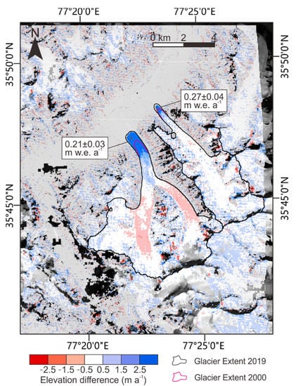
Figure 5.
Map of annual elevation change over studied area with indication of glacier mass balance. The background is a Landsat 8 panchromatic image.
A wide range of rising surface in the higher parts of two studied glaciers and other neighboring glacierized regions supported findings of mass gain in the Karakoram [36]. Due to the poor coregistration quality between HMA DEM and SRTM DEM, biases in elevation change map of off-glacier region were the major source of glacier mass change uncertainty (Figure 5). After calculating the mass changes for the two glaciers, we found that Glacier S had a mass change of 0.21 ± 0.03 m w.e. a−1, which was almost the same as Glacier A with a value of 0.27 ± 0.04 m w.e. a−1. We drew the conclusion that even though the surge broke down glacier tongue and resulted in heavy surface crevassing, it did not clearly impact the glacier mass change rate in a decadal scale.
6. Discussion
6.1. Differences between Surging and Advancing
As shown in the results, remote sensing technology can conveniently and effectively tell apart the differences between Glacier S and Glacier A in both horizontal and vertical directions. In addition, we conducted detailed topographic analysis using data from SRTM DEM (Figure 6). Although the slope of Glacier A was slightly steeper than that of Glacier S, the two glaciers both had very gentle slopes along their glacier tongues (Figure 6a). The hypsometry profiles showed that Glacier S had larger glacierized area in its lower and middle part (Figure 6b). Given that Glacier S had two tributaries converging together in the middle of its glacier tongue, it had the most ice volume in its middle part. However, this difference should be treated cautiously. Surge-type glaciers in mountain ranges did not always develop more than one tributary, such as statistical analyses of Lv et al. [27]. Therefore, this difference might not be a generic characteristic to other surge-type individuals. Judging from the surface elevation change curves, both curves had the same shape of change in the lower part, descending in the middle part, and gentle increase in the upper part (Figure 6c). What distinguished them was that the change and descending magnitude of Glacier S was bigger compared to that of Glacier A. We suggest that the shape of surface elevation change profiles for other surging and advancing glaciers would not differ significantly from those of Glacier S and Glacier A (Figure 6c). The only difference would be the zero-point position of the x axis (surface lowering) depending on regional mass balance conditions. If a glacier had a more positive mass change, the zero point of the x axis in Figure 6c would shift to the left. Otherwise, it would shift to the right.
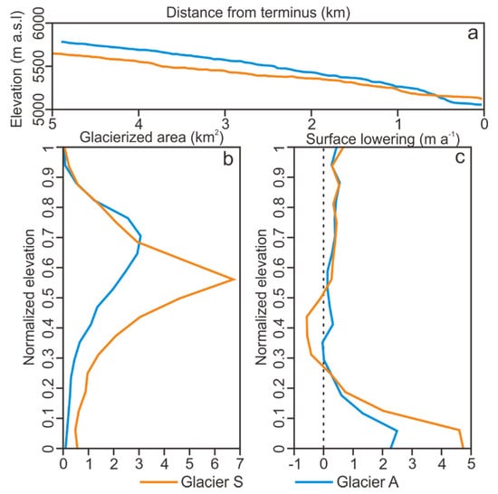
Figure 6.
Topographic and hypsometry profiles of the studied glaciers: (a) surface elevation profiles in real slope ratio measured in 2000, (b) glacier hypsometry curves measured in 2000, and (c) surface elevation change curves between 2000 and 2015.
As a surge-type glacier, Glacier S had a similar motion evolution with other surging glaciers in High Mountain Asia [15,33]. We found that the stable motion pattern of Glacier A was intriguingly different from that of advancing ones in the eastern Pamir [27]. Comparing to the period of 1999–2002, the advancing glaciers in the eastern Pamir experienced an obvious acceleration in their surface velocities in the period of 2013–2016. As a transition zone from the Karakoram positive mass balance to the western Pamir negative mass balance, the eastern Pamir had also undergone a net mass gain since the 21st century which led to the acceleration of glacial velocity [73]. The stable motion pattern of Glacier A might suggest that the mass-gain condition in the eastern Karakoram had not strengthened or weakened since the new century. In addition to this, mass changes of Glacier S and Glacier A were nearly the same mass balance value suggesting that the existence of surge-type glaciers would not influence the calculation of regional mass balance.
Combining with the results and discussion above, three differences between surging and advancing were observed. (1) The advancing distance of a nonsurging glacier terminus has a linear relationship with time, and the change rate of a surge-type glacier terminus position varies during the surge. (2) This is mainly due to another major difference, i.e., a dramatic variation in the surface velocities of the surge-type glacier. Meanwhile, the surface velocity of the advancing glacier would not go through significant rapid change. (3) The last major difference lies in the pattern of surface elevation changes. The surge results in a decrease of surface elevation in the reservoir and an increase of surface elevation in the receiving zone, whereas the advancing glacier only has an apparent elevation increase near the terminus part. If the surge happened before the acquisition time of coregistered DEMs, the receiving zone would drop down and the reservoir would rise. This is because the ice surging to the downstream begins a stage of rapid ablation, on the contrary, the reservoir starts to accumulate and store new formed ice to prepare for the next surge event. These differences were also described in previous studies around the world e.g., [22,74,75].
The differences discussed above are the remote-sensing standards for surge identification in the mountain ranges. We recommend a robust procedure for this. At first, telling from the elevation change maps, glaciers with opposite changes along their glacier tongues are selected as potential surge-type ones. Second, historical images are visually interpreted to find further evidences of rapid terminus advance and other surface feature changes, such as looped moraine and heavy crevassing [7,34]. Finally, for the glaciers with no clear sign of surging from satellite images, annual surface velocity profiles are extracted in order to detect abnormal changes at different time [27]. The increase of glacier surface velocity is taken as the sign of surge initiation, rather than the glacier terminus advance. We suggest this identification procedure could be applied to other regions in High Mountain Asia.
6.2. Controls on the Surge of Glacier S
There were researches discussing about the controls on surge mechanism in western China [22,27]. Not fitting into well-cited thermal and hydrological classifications, the controlling process in western China changed for individuals depending on their distinct thermal conditions, hydrological conditions, and geomorphological characteristics [22].
Glacier S surged for 10 years with a 2-year initiation period and an 8-year termination period. The long active phase distinguished it from hydrologically controlled surges in Alaska [18]. Although its short initiation period also differed it from the traditional thermally controlled surges, the long duration of the active phase resembled the surges in Svalbard [19]. Limited by available satellite images around 1997, apparent seasonal variations could not be detected. Due to the harsh environment of Glacier S, we could not investigate the in situ ice and bedrock temperature before and after the surge front to provide evidence of thermal condition changes inside the glacier. Hydrologically controlled surges would experience a reduction in the water discharge, as the cavity development held the meltwater within the glaciers [18,27]. The surge of Glacier S resulted in frequent variations of outflow streams from the terminus (i.e., image of August 2002 in Figure 2), which was a result of alternations in water delivery system during the surge. Although we could not observe such changes before the surge, its reservoir zone mainly locates in the valley implicating a hydrologic process during the surge initiation phase. Previous research also suggested that surges in the Karakoram are triggered by a blend of thermal and hydrological controls [22].
Glacier S and Glacier A had nearly the same aspects meaning the flow directions might not be the potential controls on surge events. It was previously demonstrated to be the case by research in the Yukon territory [74]. Although long glaciers have a greater probability to surge than short glaciers [74], the lengths of Glacier S (10.37 km) and Glacier A (9.83 km) did not differ too much (Table 1). The slope of Glacier S is slightly lower than Glacier A (Table 1 and Figure 6a). In the Yukon territory and the Novaya Zemlya, surge-type glaciers also tend to have lower slopes than nonsurging glaciers [74,75,76]. Another morphological feature of Glacier S is that it has two tributaries converging into one glacier tongue. This feature provides an advantage of gaining ice mass in the upstream and also suggests thicker ice in the main tongue. The ability of storing large amount of ice in the reservoir is essential for a surge-type glacier [11]. Glaciers in the Kingata Mountains with multiple tributaries and larger receiving zones, such as Glacier E1, E11, and E13, were also more liable to surge [27]. Thus, we suggest morphology could have a control on the formation of the surge of Glacier S.
Therefore, we suggest that both thermal and hydrological condition changes could play a role in the surge process of Glacier S. Its unique geomorphological characteristics may also control the surge to some extent.
Further, we investigated historical temperature records from 1961 to 2010 of five surrounding meteorological stations from GHCNm (Figure 7). As shown in Figure 1, Pishan, Hotan, and Shache are located in the Tarim Basin and Shiquanhe-1 and Shiquanhe-2 are located in the Tibet Plateau. These five stations are the nearest ones to our studied area. An increasing trend in mean monthly temperature could be detected from each diagram. The Tarim Basin and the Tibet Plateau were both suffering from the global warming (temperature increased by 1.4–1.9 °C from 1961 to 2010), and the Karakoram between them would very likely to be in the same situation. Even though previous studies had an agreement on that mountain glaciers in western China are more sensitive to precipitation changes than temperature changes [77,78,79], the warming in regional climate could have an impact on the thermal conditions within and beneath the glacier resulting in changes of thermal regime. Considering the discussion above, we suggest the regional warming trend has the potential to increase the instability of Glacier S and possibility of surge occurrence in this region.
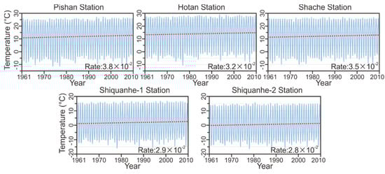
Figure 7.
Mean monthly temperature records from GHCNm of five surrounding meteorological stations from 1961 to 2010. Their tendencies are shown in red dashed lines. The unit of change rate is °C a−1.
7. Conclusions
Through a detailed investigation using remote sensing, we studied the temporal and spatial changes for a surging glacier and an advancing glacier in the eastern Karakoram from 1995 to 2019. Three major differences between them were observed: (1) the profiles of their terminus position evolution had different change patterns; (2) the surging glacier experienced a dramatic fluctuation in the surface velocities during and after the event; and (3) surface elevation of the surging glacier decreased in the reservoir and increased in the receiving zone, while the advancing glacier only had an obvious elevation increase over its terminus part. These differences can be regarded as standards for surge identification in mountain ranges. Combining with meteorological data, we discussed possible controls on the surge occurrence. Both thermal and hydrological condition variations could play a role in the surge, in addition, geomorphological characteristics and increasing warming trend could also contribute to some extent. Distinguishing glaciers between surging and advancing exactly would be a vital premise to study how climate change impact on the glacial motion variations and the regional mass changes in High Mountain Asia in the future.
Supplementary Materials
The supplementary table is available online at https://www.mdpi.com/2072-4292/12/14/2297/s1, Table S1: summary of remote sensing data used in this study.
Author Contributions
H.G., X.L., G.L., and M.L. designed this study. M.L. and K.W. conducted all data processing and visualization. J.Y. and Z.R. helped in investigation, data interpretation, and validation. M.L. and S.Y. wrote this paper. All authors played a role in review and editing this paper. All authors have read and agreed to the published version of the manuscript.
Funding
This research was funded by the Key Research Program of Frontier Sciences, Chinese Academy of Sciences [QYZDY-SSW-DQC026], the Strategic Priority Research Program of the Chinese Academy of Sciences [XDA19070202], and the National Natural Science Foundation of China [41590853].
Acknowledgments
We greatly thank all the organizations and departments for providing data used in this study. All satellite images were provided by the USGS EROS (http://glovis.usgs.gov) and Google Earth. SRTM DEM and HMA DEM were, respectively, achieved from USGS EarthExplorer (https://earthexplorer.usgs.gov) and NASA Earthdata (https://earthdata.nasa.gov). RGI version 6.0 data was downloaded from GLIMS (https://glims.org). GHCNm version 4 data was acquired from NOAA (http://ncdc.noaa.gov). We also thank three anonymous reviewers for their constructive comments on this paper.
Conflicts of Interest
The authors declare no conflict of interest.
References
- Gardner, A.S.; Moholdt, G.; Cogley, J.G.; Wouters, B.; Arendt, A.A.; Wahr, J.; Berthier, E.; Hock, R.; Pfeffer, W.T.; Kaser, G.; et al. A reconciled estimate of glacier contributions to sea level rise: 2003 to 2009. Science 2013, 340, 852. [Google Scholar] [CrossRef] [PubMed]
- Meier, M.F.; Dyurgerov, M.B.; Rick, U.K.; O’Neel, S.; Pfeffer, W.T.; Anderson, R.S.; Anderson, S.P.; Glazovsky, A.F. Glaciers dominate eustatic sea-level rise in the 21st century. Science 2007, 317, 1064. [Google Scholar] [CrossRef]
- Oerlemans, J. Quantifying global warming from the retreat of glaciers. Science 1994, 264, 243. [Google Scholar] [CrossRef]
- Haemmig, C.; Huss, M.; Keusen, H.; Hess, J.; Wegmüller, U.; Ao, Z.; Kulubayi, W. Hazard assessment of glacial lake outburst floods from Kyagar glacier, Karakoram mountains, China. Ann. Glaciol. 2014, 55, 34–44. [Google Scholar] [CrossRef]
- Jiskoot, H.; Murray, T.; Boyle, P. Controls on the distribution of surge-type glaciers in Svalbard. J. Glaciol. 2000, 46, 412–422. [Google Scholar] [CrossRef]
- Clarke, G.K.C. Fast glacier flow: Ice streams, surging, and tidewater glaciers. J. Geophys. Res. Solid Earth 1987, 92, 8835–8841. [Google Scholar] [CrossRef]
- Sevestre, H.; Benn, D.I. Climatic and geometric controls on the global distribution of surge-type glaciers: Implications for a unifying model of surging. J. Glaciol. 2015, 61, 646–662. [Google Scholar] [CrossRef]
- Meier, M.F.; Post, A. What are glacier surges? Can. J. Earth Sci. 1969, 6, 807–817. [Google Scholar] [CrossRef]
- Singh, V.P.; Singh, P.; Bishop, M.P.; Björnsson, H.; Haritashya, U.K.; Haeberli, W.; Oerlemans, J.; Shroder, J.F.; Tranter, M. Encyclopedia of Snow, Ice and Glaciers, 1st ed.; Springer: Dordrecht, The Netherlands, 2011; pp. 415–428. [Google Scholar]
- Raymond, C.F. How do glaciers surge? A review. J. Geophys. Res. Solid Earth 1987, 92, 9121–9134. [Google Scholar] [CrossRef]
- Harrison, W.D.; Post, A.S. How much do we really know about glacier surging? Ann. Glaciol. 2003, 36, 1–6. [Google Scholar] [CrossRef]
- Kargel, J.S.; Abrams, M.J.; Bishop, M.P.; Bush, A.; Hamilton, G.; Jiskoot, H.; Kääb, A.; Kieffer, H.H.; Lee, E.M.; Paul, F.; et al. Multispectral imaging contributions to global land ice measurements from space. Remote Sens. Environ. 2005, 99, 187–219. [Google Scholar] [CrossRef]
- Dunse, T.; Schellenberger, T.; Hagen, J.O.; Kääb, A.; Schuler, T.V.; Reijmer, C.H. Glacier-surge mechanisms promoted by a hydro-thermodynamic feedback to summer melt. Cryosphere 2015, 9, 197–215. [Google Scholar] [CrossRef]
- Gladstone, R.; Schäfer, M.; Zwinger, T.; Gong, Y.; Strozzi, T.; Mottram, R.; Boberg, F.; Moore, J.C. Importance of basal processes in simulations of a surging Svalbard outlet glacier. Cryosphere 2014, 8, 1393–1405. [Google Scholar] [CrossRef]
- Bhambri, R.; Hewitt, K.; Kawishwar, P.; Pratap, B. Surge-type and surge-modified glaciers in the Karakoram. Sci. Rep. 2017, 7, 15391. [Google Scholar] [CrossRef] [PubMed]
- Frappé, T.P.; Clarke, G.K.C. Slow surge of Trapridge Glacier, Yukon Territory, Canada. J. Geophys. Res. Earth Surf. 2007, 112. [Google Scholar] [CrossRef]
- Clarke, G.K.C.; Collins, S.G.; Thompson, D.E. Flow, thermal structure, and subglacial conditions of a surge-type glacier. Can. J. Earth Sci. 1984, 21, 232–240. [Google Scholar] [CrossRef]
- Kamb, B.; Raymond, C.F.; Harrison, W.D.; Engelhardt, H.; Echelmeyer, K.A.; Humphrey, N.; Brugman, M.M.; Pfeffer, T. Glacier surge mechanism: 1982–1983 surge of variegated glacier, Alaska. Science 1985, 227, 469. [Google Scholar] [CrossRef]
- Fowler, A.C.; Murray, T.; Ng, F.S.L. Thermally controlled glacier surging. J. Glaciol. 2001, 47, 527–538. [Google Scholar] [CrossRef]
- Burgess, E.W.; Forster, R.R.; Larsen, C.F.; Braun, M. Surge dynamics on Bering Glacier, Alaska, in 2008–2011. Cryosphere 2012, 6, 1251–1262. [Google Scholar] [CrossRef]
- Björnsson, H. Hydrological characteristics of the drainage system beneath a surging glacier. Nature 1998, 395, 771–774. [Google Scholar] [CrossRef]
- Quincey, D.J.; Glasser, N.F.; Cook, S.J.; Luckman, A. Heterogeneity in Karakoram glacier surges. J. Geophys. Res. Earth Surf. 2015, 120, 1288–1300. [Google Scholar] [CrossRef]
- Lingle, C.S.; Fatland, D.R. Does englacial water storage drive temperate glacier surges? Ann. Glaciol. 2003, 36, 14–20. [Google Scholar] [CrossRef]
- Turrin, J.; Forster, R.R.; Larsen, C.; Sauber, J. The propagation of a surge front on Bering Glacier, Alaska, 2001–2011. Ann. Glaciol. 2013, 54, 221–228. [Google Scholar] [CrossRef]
- Murray, T.; Stuart, G.W.; Miller, P.J.; Woodward, J.; Smith, A.M.; Porter, P.R.; Jiskoot, H. Glacier surge propagation by thermal evolution at the bed. J. Geophys. Res. Solid Earth 2000, 105, 13491–13507. [Google Scholar] [CrossRef]
- Clarke, G.K.C. Thermal Regulation of Glacier Surging. J. Glaciol. 1976, 16, 231–250. [Google Scholar] [CrossRef]
- Lv, M.; Guo, H.; Lu, X.; Liu, G.; Yan, S.; Ruan, Z.; Ding, Y.; Quincey, D.J. Characterizing the behaviour of surge- and non-surge-type glaciers in the Kingata Mountains, eastern Pamir, from 1999 to 2016. Cryosphere 2019, 13, 219–236. [Google Scholar] [CrossRef]
- Tarr, R.S.; Martin, L. Alaskan glacier studies of the National Geographic Society in the Yakutat Bay. In Prince William Sound and Lower Copper River Regions; National Geographic Society: Washington, DC, USA, 1914; p. 498. [Google Scholar]
- Post, A. Distribution of surging glaciers in western North America. J. Glaciol. 1969, 8, 229–240. [Google Scholar] [CrossRef]
- Hamilton, G.S.; Dowdeswell, J.A. Controls on glacier surging in Svalbard. J. Glaciol. 1996, 42, 157–168. [Google Scholar] [CrossRef]
- Jiskoot, H.; Boyle, P.; Murray, T. The incidence of glacier surging in Svalbard: Evidence from multivariate statistics. Comput. Geosci. 1998, 24, 387–399. [Google Scholar] [CrossRef]
- Barrand, N.E.; Murray, T. Multivariate controls on the incidence of glacier surging in the Karakoram Himalaya. Arc. Antarct. Alp. Res. 2006, 38, 489–498. [Google Scholar] [CrossRef]
- Quincey, D.J.; Braun, M.; Glasser, N.F.; Bishop, M.P.; Hewitt, K.; Luckman, A. Karakoram glacier surge dynamics. Geophys. Res. Lett. 2011, 38. [Google Scholar] [CrossRef]
- Copland, L.; Sylvestre, T.; Bishop, M.P.; Shroder, J.F.; Seong, Y.B.; Owen, L.A.; Bush, A.; Kamp, U. Expanded and Recently Increased Glacier Surging in the Karakoram. Arc. Antarct. Alp. Res. 2011, 43, 503–516. [Google Scholar] [CrossRef]
- Hewitt, K. Glacier surges in the Karakoram Himalaya (Central Asia). Can. J. Earth Sci. 1969, 6, 1009–1018. [Google Scholar] [CrossRef]
- Farinotti, D.; Immerzeel, W.W.; de Kok, R.J.; Quincey, D.J.; Dehecq, A. Manifestations and mechanisms of the Karakoram glacier Anomaly. Nat. Geosci. 2020, 13, 8–16. [Google Scholar] [CrossRef] [PubMed]
- Zemp, M.; Huss, M.; Thibert, E.; Eckert, N.; McNabb, R.; Huber, J.; Barandun, M.; Machguth, H.; Nussbaumer, S.U.; Gärtner-Roer, I.; et al. Global glacier mass changes and their contributions to sea-level rise from 1961 to 2016. Nature 2019. [Google Scholar] [CrossRef] [PubMed]
- Rankl, M.; Kienholz, C.; Braun, M. Glacier changes in the Karakoram region mapped by multimission satellite imagery. Cryosphere 2014, 8, 977–989. [Google Scholar] [CrossRef]
- Bolch, T.; Kulkarni, A.; Kääb, A.; Huggel, C.; Paul, F.; Cogley, J.G.; Frey, H.; Kargel, J.S.; Fujita, K.; Scheel, M.; et al. The State and Fate of Himalayan Glaciers. Science 2012, 336, 310. [Google Scholar] [CrossRef] [PubMed]
- Cogley, G. No ice lost in the Karakoram. Nat. Geosci. 2012, 5, 305–306. [Google Scholar] [CrossRef]
- Dehecq, A.; Gourmelen, N.; Gardner, A.S.; Brun, F.; Goldberg, D.; Nienow, P.W.; Berthier, E.; Vincent, C.; Wagnon, P.; Trouvé, E. Twenty-first century glacier slowdown driven by mass loss in High Mountain Asia. Nat. Geosci. 2019, 12, 22–27. [Google Scholar] [CrossRef]
- Rashid, I.; Abdullah, T.; Glasser, N.F.; Naz, H.; Romshoo, S.A. Surge of Hispar Glacier, Pakistan, between 2013 and 2017 detected from remote sensing observations. Geomorphology 2017, 303, 410–416. [Google Scholar] [CrossRef]
- Yasuda, T.; Furuya, M. Dynamics of surge-type glaciers in West Kunlun Shan, Northwestern Tibet. J. Geophys. Res. Earth Surf. 2015, 120, 2393–2405. [Google Scholar] [CrossRef]
- Yan, J.; Lv, M.; Ruan, Z.; Yan, S.; Liu, G. Evolution of surge-type glaciers in the Yangtze River headwater using multi-source remote sensing data. Remote Sens. 2019, 11. [Google Scholar] [CrossRef]
- Liu, G.; Guo, H.; Yan, S.; Song, R.; Ruan, Z.; Lv, M. Revealing the surge behaviour of the Yangtze River headwater glacier during 1989–2015 with TanDEM-X and Landsat images. J. Glaciol. 2017, 63, 382–386. [Google Scholar] [CrossRef][Green Version]
- Luckman, A.; Quincey, D.; Bevan, S. The potential of satellite radar interferometry and feature tracking for monitoring flow rates of Himalayan glaciers. Remote Sens. Environ. 2007, 111, 172–181. [Google Scholar] [CrossRef]
- Scherler, D.; Leprince, S.; Strecker, M.R. Glacier-surface velocities in alpine terrain from optical satellite imagery—Accuracy improvement and quality assessment. Remote Sens. Environ. 2008, 112, 3806–3819. [Google Scholar] [CrossRef]
- Pfeffer, W.T.; Arendt, A.A.; Bliss, A.; Bolch, T.; Cogley, J.G.; Gardner, A.S.; Hagen, J.; Hock, R.; Kaser, G.; Kienholz, C.; et al. The Randolph Glacier Inventory: A globally complete inventory of glaciers. J. Glaciol. 2014, 60, 537–552. [Google Scholar] [CrossRef]
- Shean, D.E.; Alexandrov, O.; Moratto, Z.M.; Smith, B.E.; Joughin, I.R.; Porter, C.; Morin, P. An automated, open-source pipeline for mass production of digital elevation models (DEMs) from very-high-resolution commercial stereo satellite imagery. ISPRS J. Photogramm. Remote Sens. 2016, 116, 101–117. [Google Scholar] [CrossRef]
- Nuth, C.; Kääb, A. Co-registration and bias corrections of satellite elevation data sets for quantifying glacier thickness change. Cryosphere 2011, 5, 271–290. [Google Scholar] [CrossRef]
- Liu, S.; Yao, X.; Guo, W.; Xu, J.; Shangguan, D.; Wei, J.; Bao, W.; Wu, L. The contemporary glaciers in china based on the second Chinese glacier inventory. Acta Geogr. Sin. 2015, 70, 3–16. [Google Scholar] [CrossRef]
- Haireti, A.; Tateishi, R.; Alsaaideh, B.; Gharechelou, S. Multi-criteria technique for mapping of debris-covered and clean-ice glaciers in the Shaksgam valley using Landsat TM and ASTER GDEM. J. Mt. Sci. 2016, 13, 703–714. [Google Scholar] [CrossRef]
- Shi, Y.; Liu, C.; Kang, E. The glacier inventory of China. Ann. Glaciol. 2009, 50, 1–4. [Google Scholar] [CrossRef]
- Zhang, X. Investigation of glacier bursts of the Yarkant River in Xinjiang, China. Ann. Glaciol. 1992, 16, 135–139. [Google Scholar] [CrossRef]
- Sinha, R.; Ravindra, R. Earth System Processes and Disaster Management; Springer: Berlin/Heidelberg, German, 2013. [Google Scholar] [CrossRef]
- Mason, K. The Shaksgam valley and Aghil range. Geogr. J. 1927, 69, 289–323. [Google Scholar] [CrossRef]
- Immerzeel, W.W.; Pellicciotti, F.; Shrestha, A.B. Glaciers as a proxy to quantify the spatial distribution of precipitation in the Hunza Basin. Mt. Res. Dev. 2012, 32, 30–38. [Google Scholar] [CrossRef]
- Yao, T.; Thompson, L.; Yang, W.; Yu, W.; Gao, Y.; Guo, X.; Yang, X.; Duan, K.; Zhao, H.; Xu, B.; et al. Different glacier status with atmospheric circulations in Tibetan Plateau and surroundings. Nat. Clim. Chang. 2012, 2, 663. [Google Scholar] [CrossRef]
- Gardelle, J.; Berthier, E.; Amaud, Y.; Kääb, A. Region-wide glacier mass balances over the Pamir-Karakoram-Himalaya during 1999–2011. Cryosphere 2013, 7, 1263–1286. [Google Scholar] [CrossRef]
- Farr, T.G.; Rosen, P.A.; Caro, E.; Crippen, R.; Duren, R.; Hensley, S.; Kobrick, M.; Paller, M.; Rodriguez, E.; Roth, L.; et al. The shuttle radar topography mission. Rev. Geophys. 2007, 45. [Google Scholar] [CrossRef]
- Menne, M.J.; Williams, C.N.; Gleason, B.E.; Rennie, J.J.; Lawrimore, J.H. The global historical climatology network monthly temperature dataset, version 4. J. Clim. 2018, 31, 9835–9854. [Google Scholar] [CrossRef]
- Hall, D.K.; Bayr, K.J.; Schöner, W.; Bindschadler, R.A.; Chien, J.Y.L. Consideration of the errors inherent in mapping historical glacier positions in Austria from the ground and space (1893–2001). Remote Sens. Environ. 2003, 86, 566–577. [Google Scholar] [CrossRef]
- Paul, F.; Barrand, N.E.; Baumann, S.; Berthier, E.; Bolch, T.; Casey, K.; Fre, H.; Joshi, S.P.; Konovalov, V.; le Bris, R.; et al. On the accuracy of glacier outlines derived from remote-sensing data. Ann. Glaciol. 2013, 54, 171–182. [Google Scholar] [CrossRef]
- Leprince, S.; Barbot, S.; Ayoub, F.; Avouac, J. Automatic and precise orthorectification, coregistration, and subpixel correlation of satellite images, application to ground deformation measurements. IEEE Trans. Geosci. Remote Sens. 2007, 45, 1529–1558. [Google Scholar] [CrossRef]
- Rignot, E.; Echelmeyer, K.; Krabill, W. Penetration depth of interferometric synthetic-aperture radar signals in snow and ice. Geophys. Res. Lett. 2001, 28, 3501–3504. [Google Scholar] [CrossRef]
- Kääb, A.; Berthier, E.; Nuth, C.; Gardelle, J.; Arnaud, Y. Contrasting patterns of early twenty-first-century glacier mass change in the Himalayas. Nature 2012, 488, 495. [Google Scholar] [CrossRef]
- Ragettli, S.; Bolch, T.; Pellicciotti, F. Heterogeneous glacier thinning patterns over the last 40 years in Langtang Himal, Nepal. Cryosphere 2016, 10, 2075–2097. [Google Scholar] [CrossRef]
- Huss, M. Density assumptions for converting geodetic glacier volume change to mass change. Cryosphere 2013, 7, 877–887. [Google Scholar] [CrossRef]
- Fischer, M.; Huss, M.; Hoelzle, M. Surface elevation and mass changes of all Swiss glaciers 1980–2010. Cryosphere 2015, 9, 525–540. [Google Scholar] [CrossRef]
- Rolstad, C.; Haug, T.; Denby, B. Spatially integrated geodetic glacier mass balance and its uncertainty based on geostatistical analysis: Application to the western Svartisen ice cap, Norway. J. Glaciol. 2009, 55, 666–680. [Google Scholar] [CrossRef]
- Bolch, T.; Pieczonka, T.; Benn, D.I. Multi-decadal mass loss of glaciers in the Everest area (Nepal Himalaya) derived from stereo imagery. Cryosphere 2011, 5, 349–358. [Google Scholar] [CrossRef]
- Zhou, Y.; Hu, J.; Li, Z.; Li, J.; Zhao, R.; Ding, X. Quantifying glacier mass change and its contribution to lake growths in central Kunlun during 2000–2015 from multi-source remote sensing data. J. Hydrol. 2019, 570, 38–50. [Google Scholar] [CrossRef]
- Brun, F.; Berthier, E.; Wagnon, P.; Kääb, A.; Treichler, D. A spatially resolved estimate of High Mountain Asia glacier mass balances from 2000 to 2016. Nat. Geosci. 2017, 10, 668. [Google Scholar] [CrossRef]
- Clarke, G.K.C.; Schmok, J.P.; Ommanney, C.S.L.; Collins, S.G. Characteristics of surge-type glaciers. J. Geophys. Res. Solid Earth 1986, 91, 7165–7180. [Google Scholar] [CrossRef]
- Grant, K.L.; Stokes, C.R.; Evans, I.S. Identification and characteristics of surge-type glaciers on Novaya Zemlya, Russian Arctic. J. Glaciol. 2009, 55, 960–972. [Google Scholar] [CrossRef]
- Clarke, G.K.C. Length, width and slope influences on glacier surging. J. Glaciol. 1991, 37, 236–246. [Google Scholar] [CrossRef][Green Version]
- Shi, Y. Characteristics of late Quaternary monsoonal glaciation on the Tibetan Plateau and in East Asia. Quat. Int. 2002, 97–98, 79–91. [Google Scholar] [CrossRef]
- Seong, Y.B.; Owen, L.A.; Yi, C.; Finkel, R.C.; Schoenbohm, L. Geomorphology of anomalously high glaciated mountains at the northwestern end of Tibet: Muztag Ata and Kongur Shan. Geomorphology 2009, 103, 227–250. [Google Scholar] [CrossRef]
- Holzer, N.; Vijay, S.; Yao, T.; Xu, B.; Buchroithner, M.; Bolch, T. Four decades of glacier variations at Muztagh Ata (eastern Pamir): A multi-sensor study including Hexagon KH-9 and Pléiades data. Cryosphere 2015, 9, 2071–2088. [Google Scholar] [CrossRef]
© 2020 by the authors. Licensee MDPI, Basel, Switzerland. This article is an open access article distributed under the terms and conditions of the Creative Commons Attribution (CC BY) license (http://creativecommons.org/licenses/by/4.0/).