Abstract
Many software packages are designed to process 3D geometric data, although very few are designed to deal with 3D thermal models of buildings over time. The software 3D Temporal Thermal Analysis (3D-TTA) has been created in order to visualize, explore and analyze these 3D thermal models. 3D-TTA is composed of three modules. In the first module, the temperature of any part of the building can be explored in a 3D visual framework. The user can also conduct separate analyses of structural elements, such as walls, ceilings and floors. The second module evaluates the thermal evolution of the building over time. A multi-temporal 3D thermal model, composed of a set of thermal models taken at different times, is handled here. The third module incorporates several assessment tools, such as the identification of representative thermal regions on structural elements and the comparison between real and simulated (i.e., obtained from energy simulation tools) thermal models. The potential scope of this software and its applications within the field of energy efficiency are presented in various case studies at the end of the paper.
1. Introduction
Nowadays, the 3D digitization of indoors/outdoors building is extensively used in the fields of Architecture, Engineering and Construction (AEC). This has led to the development of multiple robotic platforms for the digitization of buildings in recent years [1]. Nevertheless, the point cloud models that are generated are almost exclusively used to evaluate the geometric features of a building [2,3,4,5]. Although the geometric data is of great importance to the assessment of the state of the building and its conservation, other sorts of data and evaluations regarding buildings are also required. Among other applications, this information can be used to detect the thermal features of the building, with which its energy efficiency and zones with special thermal features (e.g., thermal bridges and energy losses) can be assessed [6].
Currently, thermal imaging cameras can be used to perform a thermal assessment of a building, by recording the temperatures of a limited area within their field of view. Thermal imaging camera manufacturers market their own tools for the analysis of these images [7,8,9]. Likewise, 3D laser scanner manufacturers—such as [10,11,12]—also offer their own software tools for point-cloud visualization and evaluation. There are also applications that are not strictly focused on the assessment of buildings (e.g., [13,14]), which are also supplied with a wide range of tools. However, these applications may be of little use to AEC professionals because their functionalities are neither adapted to architectural nor to civil engineering applications. Recently, new tools for the analysis of point clouds in an AEC context have been placed on the market ([15,16,17]), and some of the common software tools used by architects and civil engineers now include new functionalities that handle thermal information [18,19,20].
Due to the interest in obtaining and analyzing the thermal information of buildings in a 3D context, different methods ([21,22,23]), systems ([24,25,26]) and even autonomous thermal scanning robots ([27,28]), which obtain 3D thermal models of buildings, have been developed in the last years.
As discussed above, several tools that are marketed in the field of AEC explore 2D thermal images and process point clouds, but there are no specific tools that deal with 3D thermal models of buildings. The user can import point-cloud coordinates with certain tools, such as [14,15], together with associated values. These values are not the real temperature, but relative measures of the temperature, which are visualized according to a specific color palette.
Recently, new developments have come online that address the evaluation of thermal information inserted in 3D data. Nüchter et al. developed a tool called The 3D Toolkit [29] that provides various 3D thermal point-cloud functionalities. The visualizer can show the reflectance, color or temperature of the point cloud. Thus, the user can choose among different point cloud representations and localize energy leaks. Moghadam et al. presented Spectra [30], which contains a set of tools for multispectral fusion and visualization. Both the thermal and visual spectrum can be simultaneously modeled on a 3D mesh with this software. However, rather than buildings, Spectra is designed for smaller-scale scenarios, such as air-conditioning and compressor units. The visualization options of the tool can highlight regions with extreme temperatures, among other options. In [31], the authors presented a software for the ex situ inspection of building interiors using 3D data, previously acquired with the IMAS (Indoor Multi-sensor Acquisition System) digitalization platform. The scene can be inspected by carrying out an immersive virtual navigation, in which the user can see: the point cloud and the RGB (Red, Green, Blue) images, the thermal images, the luminance, the temperature and the humidity while navigating within IMAS. Natephra et al. [32] proposed a system for the eventual evaluation of the thermal comfort conditions at different locations within the building. The authors used commercial tools (i.e., Rhinoceros [33], together with the plug-in Grasshopper [34]) to visualize the evolution of thermal information over time, in the context of Building Information Modeling (BIM). In [35], a method was presented for the automatic analysis and visualization of the deviations between the energy status of a building and the expected 3D spatial-thermal simulated model. The energetic model of the building was obtained by using a set of thermal images, and the simulated model was calculated by means of a Computation Fluid Dynamics (CFD) analysis. Finally, a 3D virtual environment was used to superimpose both models, highlighting the areas identified as potentially problematic. Table 1 shows a comparison of the aforementioned software tools. The columns of this table refer to: the data sources, dealing with temporal thermal data, 3D thermal data processing algorithms, functionalities in a thermal context, the kind of software (commercial/research) and applications in the AEC thermal context.

Table 1.
Software technologies for 3D point clouds and 3D thermal data. (Abbreviations. 3D-T = 3D thermal data, 2D-T = 2D thermal data, C = Commercial, R = Research).
In this article, we present 3D-TTA, a tool for the visualization and exploration of 3D thermal models of buildings, which offers a set of functionalities designed to facilitate the assessment of these models. Compared with the above-mentioned tools, we can highlight several major contributions:
- 3D-TTA deals with temporal thermal models in 3D environments, which is totally novel in the state of the art. To date, variable time has neither been introduced into 3D thermal models, nor has it been considered in the analysis phase.
- 3D-TTA includes original 3D thermal data processing algorithms—some based on temporal thermal data—that can efficiently identify and delimit zones with different thermal behaviors over time.
- 3D-TTA can compare real and simulated thermal models of buildings, providing a useful calibration tool for architects and engineers.
2. 3D-TTA Software
The main objective of the 3D-TTA tool is to monitor 3D thermal models of building interiors. It provides Architecture, Engineering and Construction professionals with the possibility of visualizing and exploring thermal behavior at different times. It could therefore be a valuable tool with which to detect regions that have special thermal features with a high degree of precision, such as moisture and thermal bridges, and to position them in a 3D model of the building.
The 3D-TTA inputs are 3D thermal point clouds, which are collected by a 3D thermal acquisition system. Figure 1a shows the 3D thermal acquisition system used for this study, comprising a 3D laser scanner Riegl Vz-400, a Nikon D90 RGB camera and a FLIR Ax5 thermal camera [24]. A view of the 3D thermal model of a building obtained from this system is shown in Figure 1b.
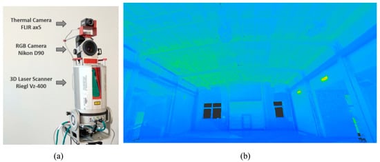
Figure 1.
(a) 3D thermal acquisition system composed of a 3D scanner, an RGB camera and a thermal camera. (b) Example of thermal point cloud of a building.
3D-TTA is divided into three different modules. The first module deals with the visualization and exploration of the 3D building thermal model, which can later be segmented into the structural elements (SEs) that constitute the building. The outputs of this module are the inputs for the remaining modules. With the second module, the user can analyze the thermal evolution of the building over time, and the third module is used to implement new thermal-data processing algorithms.
Modules 1 and 2 were developed in C++, based on the Qt framework [36], using the PCL [37] and OpenCV [38] libraries, and Module 3 was implemented using Matlab and subsequently integrated into the whole tool. The diagram in Figure 2 illustrates the connection between the three modules. The following sections will provide a more in-depth explanation of each module.
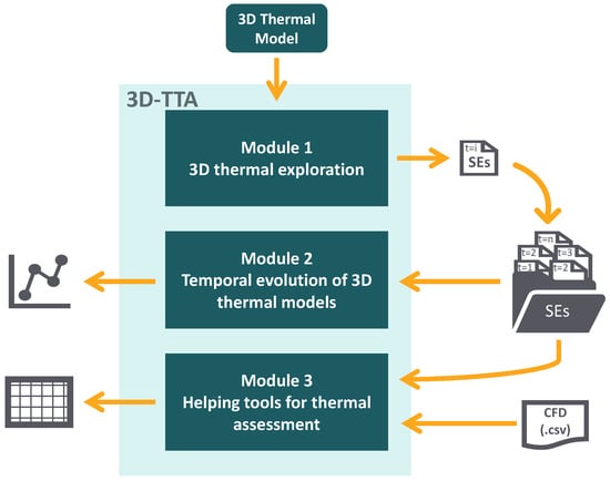
Figure 2.
Main modules of 3D-TTA.
2.1. Module 1: 3D Thermal Exploration
Module 1 comprises several tools with which to explore 3D thermal models of buildings at any one particular time. The exploration ranges from the generation of the building blueprint to the extraction of thermal orthoimages of structural elements. Figure 3 shows a diagram with the different tools and functionalities of Module 1. A brief step-by-step description of the module is presented below.
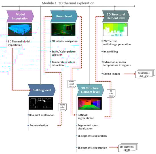
Figure 3.
Diagram of the tools and functionalities of Module 1.
2.1.1. 3D Exploration: Building Level
3D-TTA imports coarse unorganized 3D thermal data, i.e., point clouds containing 3D coordinates and temperatures. This is a raw text file organized into four columns that is selected at the beginning of the session.
After opening the data file, the total thermal point cloud of the building can be seen as a large unorganized point cloud. Nevertheless, this software has been created to explore different parts of the building in greater detail, which have been organized into rooms and, afterwards, into Structural Elements.
The original 3D point cloud is therefore first processed with the objective of generating a 2D building blueprint. The process consists of extracting, from the initial point cloud, the points contained within a horizontal 40-cm wide slice, positioned midway between the maximum and the minimum Z values. These points are then projected onto the XY plane, thus creating the 2D blueprint of the building. This representation quickly displays a sharply defined overview of the building structure, with no need for the use of building layouts. The user can then move around the blueprint and select the room that is to be explored.
2.1.2. 3D Exploration: Room Level
Virtual navigation is implemented in this part of the module. The observer can move and orientate the camera in order to view the thermal point cloud from all possible perspectives and positions. The user can also orbit the whole scene around a fixed point and zoom into specific regions. The temperature scale and the color palette can be customized in the visualizer. Apart from the visual exploration and qualitative analysis via the use of a color code, the tool also shows the temperature of the regions that are selected by the user, providing mean, maximum and minimum temperatures.
2.1.3. 3D Exploration: Structural Element Level
The point cloud of any one room that is selected can subsequently be segmented into its structural elements (i.e., walls, ceiling and floor). This is an iterative process, in which plane regions are detected by applying the RANSAC algorithm [39]. An array of parameters, such as the distance threshold, the stopping threshold and the number of iterations, can be pre-set. The user can first check the results and then modify the parameters in order to obtain a precise segmentation, as each visualization depends to a great extent on the parameter values. Figure 4 shows a flowchart of the whole process.
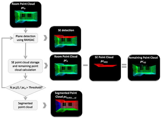
Figure 4.
Steps of the 3D segmentation process. A point cloud of the room is split into different point clouds, each representing a structural element.
Once the room has been segmented, the visualizer can show (or hide), in different colors, the resulting segments of the room. In this way, potential errors can be detected, and, if needed, the user can modify the input parameters and, once again, repeat the segmentation process. The temperature of the structural elements can likewise be separately explored, by using the same local functionalities that are found in Module 1.
2.1.4. 2D Exploration: Structural Element Level
Thermal inspections of buildings are usually carried out with a thermal camera. Since the field of view of these cameras is limited, the operator must take a large number of photos in order to cover the complete scene. The off-site evaluation, registration and segmentation of these large data volumes is a tedious process. Apart from that, it is difficult to know precisely the position of the image within the 3D model of the building. As a solution to this problem, 3D-TTA offers the possibility of extracting a single thermal image (i.e., thermal orthoimage) per each structural element of the building, by taking advantage of the aforementioned segmentation tool.
The generation of the thermal orthoimage of a structural element is illustrated in Figure 5. The first step consists in obtaining a coarse image from the point cloud corresponding to the structural element. Let SE(i) be the i-th structural element of a certain room. The segment of points P3D(i) is first projected onto the plane calculated by RANSAC, in order to generate the corresponding thermal orthoimage, I(i), thus obtaining the set P2D(i). P2D(i) is then discretized in a grid with a resolution of 1cm/pixel, thereby generating the thermal orthoimage, I0(i).
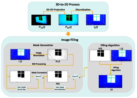
Figure 5.
Flowchart showing the generation of the thermal orthoimages of the structural elements. (Up) Generating the coarse orthoimage I0(i); (Down) Image filling algorithm.
Owing to the limited resolution of the scanner and the potential occlusion on the plane of the structural element (SE), I0(i) might contain gaps and regions without data. It is therefore necessary to implement a hole-filling algorithm that restores I0(i). This is the second step of the process.
As mentioned above, the gaps within the orthoimage can be produced by different factors, such as occlusions, an absence of data, openings on the wall and irregularities in the structural element geometry [40]. In view of the wide diversity of sizes and shapes of these holes, the user selects some filling-process parameters from a menu and then checks the results. The procedure is as follows.
We first generate an initial binary mask, M0(i), of the same size as I0(i), in which a pixel is set to 1 when it contains data and is otherwise 0. M0(i) is modified by applying morphological operations with a kernel whose size is set by the user. This process is repeated until the white pixels of the new versions of M0(i) roughly cover the area of the SE, excluding openings. The user can then manually refine the new version of the mask M0(i) in order to obtain the final mask, M(i).
The initial thermal orthoimage, I0(i), and the mask, M(i), are used in order to generate the filled thermal orthoimage, I(i), by applying the Navier–Stokes algorithm [41].
2.2. Module 2. Temporal Evolution of 3D Thermal Models
The second module focuses on analyzing the thermal evolution of the building over time. The input of this module is the set of thermal orthoimages corresponding to each structural element at different times. Note that the interval of time between orthoimages could either be minutes, hours or days. Figure 6 shows a diagram with different tools and functionalities of Module 2 divided into three blocks: SE Temporal Exploration, Thermal Characterization by regions and Graphic Analysis.
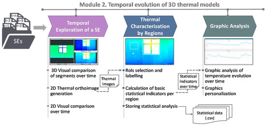
Figure 6.
Diagram of tools and functionalities of Module 2. Note: (RoI=Region of Interest).
2.2.1. Temporal Exploration of a Structural Element (SE)
Once the segmented models have been uploaded in the tool, the user can conduct an exploration and visual comparison of the thermal evolution over time. This evaluation is carried out by using both the point cloud segments and the SE thermal orthoimages at different times. For each structural element, a list of the different times at which the models were acquired is displayed. The user can then select several points in time from the list, and the corresponding orthoimages will be shown in a multi-window environment. Moreover, a different visualization option is offered to the users, which shows a temporal animation of any specific SE and its thermal variations. An operation that is performed by clicking a slider bar allows the user to visualize a sequence of thermal images at different times.
2.2.2. Thermal Characterization by Regions
In this block, the user can select different regions of a structural element that may be of interest by clicking and dragging on the corresponding orthoimage. The thermal evolution over time is then calculated for each labeled region, evaluating a set of basic statistical indicators, such as the mean, minimum and maximum temperatures. The results of this analysis can be exported to a .csv file. In this way, the evaluation results can be easily compared with local data collected with other sensors or with data that are estimated with energy simulation software.
2.2.3. Graphic Analysis
The previously calculated statistical indicators can be graphically visualized in the third block of this module. It provides thermal comparisons between regions composed of different materials or between different areas belonging to the same SE.
2.3. Module 3. Useful Tools for Thermal Assessment
The third 3D-TTA module comprises two sub-modules that implement innovative research methods for the automatic extraction of useful information from 3D thermal models: Real vs. Simulated Thermal Data, and Automatic Region Segmentation. A diagram illustrating both sub-modules is presented in Figure 7, together with the different inputs and outputs.
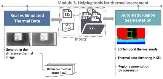
Figure 7.
Diagram of the tools and functionalities of Module 3.
2.3.1. Comparing Real and Simulated Thermal Models
The first sub-module addresses the issue of comparing real thermal data (obtained from the first module) and simulated thermal data (usually obtained from Computational Fluid Dynamics tools (CFD)). The comparison is implemented by means of a difference thermal image, which yields a quantitative evaluation of the differences between both datasets.
This sub-module has two inputs. The first input is a thermal orthoimage at any one time, t, of an SE of the building. The second input is obtained from the energy analysis software DesignBuilder. Among its other functionalities, this software conducts energy simulations of buildings by using Energy Plus as a calculation engine. A CFD simulation of the geometric model of the building at the same time, t, generates the second input of the sub-module, eventually obtaining a simulated thermal map of the SE that is selected. The thermal map is a non-uniform grid composed of a set of different sized zones, which is then exported to a .csv file. In the last stage, after a scaling algorithm procedure, the sub-module carries out a comparison between both thermal images.
2.3.2. Segmenting SEs into Smaller Regions through a Temporal Analysis of Thermal Maps
The second sub-module is focused on the automatic segmentation of structural elements into representative regions from a thermal-evolution point of view. The input to this sub-module is the set of thermal orthoimages of a structural element at different times.
The process is divided into two stages. In the first stage, the set of temporal thermal orthoimages is segmented into regions after using three different clustering methods: k-means, Gaussian Mixture Distribution and Hierarchical Clustering algorithms. The structural element is defined as a three-dimensional thermal data structure D (w × h × t) in order to perform the temporal segmentation, where w × h are references to the size of the orthoimage and t is the time. Each algorithm yields a set of segments, each characterized by a temporal temperature-prototype-vector. A consensus algorithm is then conducted. To do so, two distance metrics have been defined between the earlier methods, which evaluate, on one hand, d1, which is the overlap between the segments in the image and, on the other hand, d2, which is the Euclidean distance between the respective prototype thermal vectors. For a specific region, its associated prototype thermal vector stores the average temperature of the region over time. After the consensus, several regions of the structural element are characterized by a consensus temperature-prototype-vector.
A flowchart illustrating the whole process is presented in Figure 8. More information on this algorithm can also be found in [42].
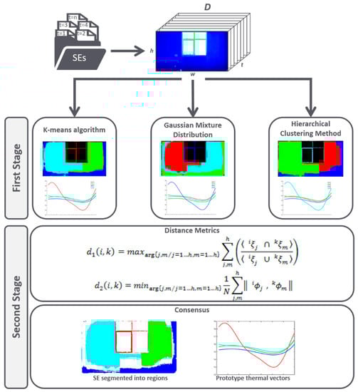
Figure 8.
Flowchart of the automatic region segmentation through a temporal analysis of the thermal maps.
3. Case Studies
In this section, representative case studies of the application of the 3D-TTA software are presented. Two 3D thermal models of two different scenarios are presented in this section. The first 3D thermal model is composed of 16 rooms and 122 million points. The model was obtained after digitizing a part of the Building Science Institute at the University of Castilla-La Mancha (UCLM) in Spain. Figure 9a shows the blueprint of the part of the building that is digitized and some pictures of different rooms. The second 3D thermal model corresponds to the 3D Visual Computing & Robotics Lab (UCLM), composed of one room and 2.5 million of points (see Figure 9b).
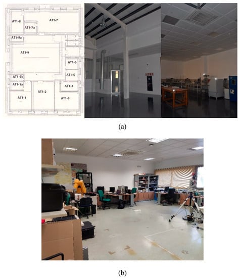
Figure 9.
(a) First scenario. Blueprint and pictures of some rooms. (b) Second scenario.
In order to analyze the thermal evolution over time of a particular wall, a scanning session was conducted in both scenarios. To do this, the scanner was placed in a fixed position, and the wall was digitalized over a period of 24 h, with a time-lapse of 30 min. Thus, a total of 48 3D thermal models of the wall was obtained.
3.1. Module 1. Results
After importing the 3D thermal model of the building in Module 1 of 3D-TTA, a coarse 2D blueprint of the building is generated, as illustrated in Figure 10a.
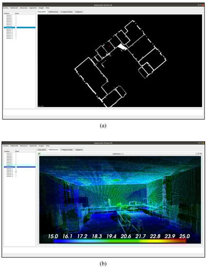
Figure 10.
3D-TTA Module 1. (a) 2D building blueprint of scenario 1. (b) Room exploration mode.
Figure 10b illustrates the “Room Exploration” mode. The viewer displays a 3D view of room #13 from scenario 1, previously selected from the blueprint. As can be seen, the warm and the cold areas are clearly distinguished in the thermal point cloud. Moreover, the options to customize the scale and the color palette make it easier to visualize thermal variations in the model.
Figure 11a shows the different colored segments that correspond to the structural elements of the room, whereas Figure 11b presents a view of the multi-window mode. In this visualization mode, each window contains the thermal point cloud of a selected structural element.
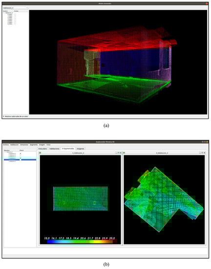
Figure 11.
3D-TTA Module 1: (a) Room segmented into structural elements in different colors. (b) Multi-window mode showing the 4-th SE of room #3 and 4-th SE of room #0 (Scenario 1).
Figure 12 presents two orthoimages corresponding to the point clouds shown in Figure 11b. Note that the orthoimage on the left has yet to be filled, whereas the orthoimage on the right was filled using the hole-filling algorithm, described in Section 2.1. It is clear that the visualization of the last image is greatly enhanced after applying the hole-filling algorithm. The user can then select different regions of the orthoimage and obtain the corresponding mean, maximum and minimum temperatures. As was mentioned in Section 2.2, these images can be exported to several formats (TXT, PNG, XML).
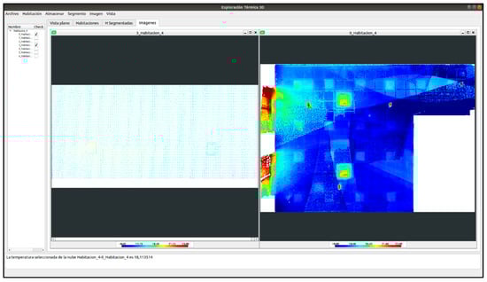
Figure 12.
3D-TTA Module 1: Visualization of two SE orthoimages of the 4-th SE of room #3 and 4-th SE of room #0 (Scenario 1). Note that the filling-hole process has not been applied to the first image.
3.2. Module 2. Results
The thermal evolution of a wall from Scenario 2 (see Figure 13a) is shown in this module. To do so, a set of 48 3D thermal models from Scenario 2 was obtained over a 24-hour time-period, with a time lapse of 30-minutes. With this dataset, the user can perform an analysis of the thermal evolution of the room over time. The data input for Module 2 is obtained by segmenting each of the 48 room models into their respective structural segments by using Module 1. Figure 13b shows a visual comparison in a multi-window environment of the temperature of the chosen wall at different times.
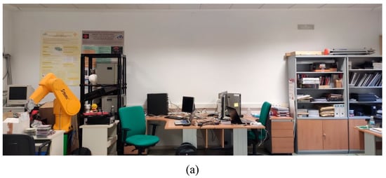
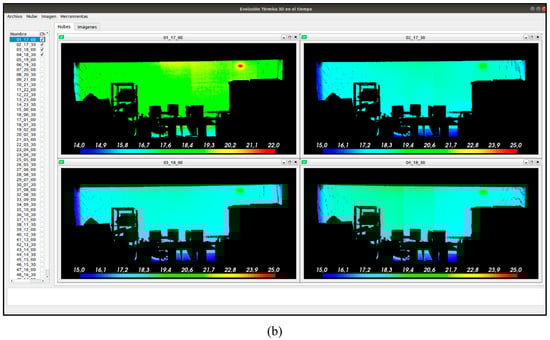
Figure 13.
(a) Wall used to illustrate the thermal evolution of the Module 2 results. (b) Thermal orthoimages for different times.
The thermal characterization per region is carried out by selecting several regions of interest (Figure 14a). For each Region of Interest (RoI), some basic statistical indicators (mean, maximum and minimum temperature) are then computed, which may also be graphically analyzed, as shown in Figure 14b.
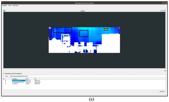
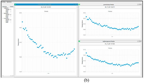
Figure 14.
3D-TTA Module 2: (a) Example of the selection and labeling of three regions. (b) Graphics of the temperature evolution over time and basic statistical indicators for each region.
3.3. Module 3.1. Results
A set of orthoimages of a wall from Scenario 1 was generated, to compare the real thermal model with the simulated thermal model. Both walls were digitized with our 3D thermal scanning system during 24 h, at 30-min intervals.
As explained in Section 2.3, the first sub-module (i.e., 3D-TTA Module 3_1) is employed to perform a comparison between the real data, obtained in our 3D thermal scanning system, and the simulated data, obtained from the energy simulation software DesignBuilder. Figure 15 shows a flowchart of this process.
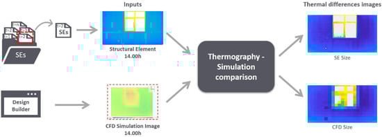
Figure 15.
Flowchart of the thermography-simulation comparison process.
In this case study, we chose the thermal orthoimage at 2 pm of a wall from Scenario 1. Figure 16b shows the user interface of this sub-module. The outputs of this comparison were two difference thermal-images of different resolutions (pixel/cm2). One of them was adapted to the original resolution of the thermal orthoimage (Figure 16b, left), and the other was adapted to the resolution of DesignBuilder (Figure 16b, right).
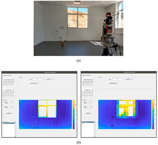
Figure 16.
3D-TTA Module 3_1: (a) Wall used to illustrate the results of Module 3.1. (b) User interface showing the difference thermal-images with different resolutions: original resolution of the thermal orthoimage (left) and resolution of DesignBuilder (right).
After observing the results, it can be stated that the differences are below 1 degree Celsius in the wall area (in blue). It can also be seen that the temperature difference is slightly greater around the lower part and sides of the wall than elsewhere. With regard to the window frame area (aluminum carpentry), the temperature differences were between 1.5 and 3 degrees Celsius, differences that increase whenever the point was closer to the center.
3.4. Module 3.2. Results
With regard to the second sub-module, we present the segmentation results for two structural elements of Scenario 2. We first obtained 48 thermal orthoimages of the walls at different times and intervals, and the algorithm then yielded the regions together with their temporal evolution over time. Figure 17 and Figure 18 show the results of this sub-module. In both scenes, the wall has been segmented into four regions. The test walls and the visualization of the segmented regions in different colors are presented in Figure 17a and Figure 18a. The black color signifies no data. Figure 17b and Figure 18b show the prototype vectors of the segmented regions.
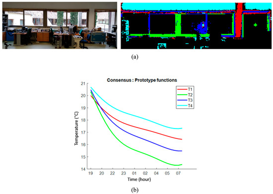
Figure 17.
3D-TTA Module 3.2: Segmentation into regions through a temporal analysis of thermal maps. (a) The test wall and the visualization of the segmented regions in different colors. (b) Corresponding prototype vectors are in the same colors.
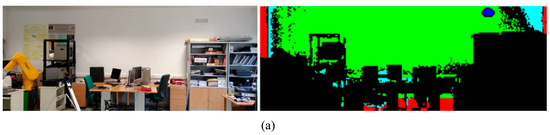
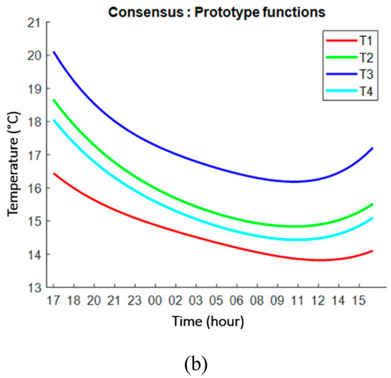
Figure 18.
3D-TTA Module 3.2: Segmentation into regions through a temporal analysis of thermal maps. (a) The test wall and visualization of the segmented regions in different colors. (b) Corresponding prototype vectors are in the same colors.
In the first case, the cyan segment is the warmest part of the wall, where the temperature decrease is slower than in the other regions. Curiously enough, the red region covers a vertical zone between the windows, which might suggest that part of the wall was constructed from a different material. The upper horizontal part in red corresponds to the roll-up blinds, which are raised. The blue and green regions are clearly located within the window frames. As expected, the temperature of the (aluminum) window follows, with a degree of thermal inertia, the outdoor temperature and decreases faster than the other segments. The difference between the blue and the red zones is probably explained by a higher or lower thermal loss, depending on whether the locking mechanisms are within the segment and on the enclosure of the window.
In the second case, a large (green) region covers most of the wall, which signifies a uniform temperature explained by the thermal inertia of the wall. The left, right and lower borderlines of the wall are clearly the coolest zones with the highest thermal inertia. Finally, the blue spot corresponds to an alarm light, the warmest segment point in the image.
4. Conclusions and Future Developments
Many of the 3D-data acquisition devices in use today are used to generate geometric models of buildings and facilities, which is very useful in the field of AEC. Additionally, a large number of related software tools, with a broad range of geometric functionalities, have been developed. Nevertheless, until now, there have been no specific applications focusing on the exploration of 3D thermal models of buildings and their analysis.
The effective export of new technologies and formats for the analysis of the thermal efficiency of buildings can be the next goal for this kind of software. The analysis can go from a study with local and static data in walls to a methodology based on the exploration and identification of problems in three-dimensional thermal models. Additionally, the data processing of 3D thermal models of entire buildings can have an appreciable impact on the world of engineering/architecture.
In this paper, the first steps have been taken in the exploitation of these technologies for the study of energy efficiency. 3D-TTA has been presented as a tool that visualizes, explores and processes 3D thermal models of buildings. Among its functionalities, 3D-TTA can be used for: the visual detection of regions with special thermal features (e.g., thermal bridges and moistures) in a 3D framework; the generation of thermal images of structural elements; the visualization of the evolution of the temperature on different structural elements and surfaces over time; and the automatic segmentation of structural elements by their thermal behavior. Moreover, the tool includes an additional module for comparisons between simulated and real thermal data.
3D-TTA is a first version that will be improved and extended to other functionalities in future versions. A great challenge consists in translating the 3D thermal model, as well as the results obtained from the different steps in the thermal analysis process, to the BIM world. This entails adapting the 3D-TTA outputs so as to introduce them into gbxml and IDF file formats. More effective algorithms that process 3D thermal point clouds must be introduced. For example, the automatic detection of thermal failures at higher levels than those used in the current 3D-TTA version (e.g., SE level) would be a very useful attribute in thermal imaging software, offering a global characterization of the building with the option of thermal evaluations of a single room, a set of rooms or a complete floor.
Author Contributions
Conceptualization, J.G., A.A., V.P. and F.J.C.; Data curation, J.G. and A.A.; Formal analysis, J.G.; Funding acquisition, A.A.; Investigation, A.A.; Methodology, J.G.; Project administration, A.A.; Resources, J.G., B.Q. and A.A.; Software, J.G.; Supervision, B.Q., V.P. and F.J.C.; Validation, J.G., A.A., V.P. and F.J.C.; Visualization, J.G., B.Q. and A.A.; Writing—original draft, B.Q.; Writing—review & editing, J.G., B.Q., A.A., V.P. and F.J.C. All authors have read and agreed to the published version of the manuscript.
Funding
This work has been financed by the European Regional Development Fund [SBPLY/19/180501/000094 project] and the Ministry of Science and Innovation [PID2019-108271RB-C31].
Acknowledgments
Thanks to the European Regional Development Fund [SBPLY/19/180501/000094 project] and to the Ministry of Science and Innovation [PID2019-108271RB-C31].
Conflicts of Interest
The authors declare no conflict of interest.
References
- Adán, A.; Quintana, B.; Prieto, S.A. Autonomous mobile scanning systems for the digitization of buildings: A review. Remote Sens. 2019, 11, 306. [Google Scholar] [CrossRef]
- Valero, E.; Adan, A.; Huber, D.; Cerrada, C. Detection, Modeling, and Classification of Moldings for Automated Reverse Engineering of Buildings from 3D Data. In Proceedings of the 28th International Symposium on Automation and Robotics in Construction (ISARC), Seoul, Korea, 29 June–2 July 2011. [Google Scholar] [CrossRef]
- Quintana, B.; Prieto, S.A.; Adán, A.; Vázquez, A.S. Semantic Scan Planning for Indoor Structural Elements of Buildings. Adv. Eng. Inform. 2016, 30, 643–659. [Google Scholar] [CrossRef]
- Macher, H.; Landes, T.; Grussenmeyer, P. From point clouds to building information models: 3D semi-automatic reconstruction of indoors of existing buildings. Appl. Sci. 2017, 7, 1030. [Google Scholar] [CrossRef]
- Wang, Q.; Kim, M.K. Applications of 3D point cloud data in the construction industry: A fifteen-year review from 2004 to 2018. Adv. Eng. Inform. 2019, 39, 306–319. [Google Scholar] [CrossRef]
- Brooke, C. Thermal imaging for the archaeological investigation of historic buildings. Remote Sens. 2018, 10, 1401. [Google Scholar] [CrossRef]
- Fluke SmartView. Available online: https://www.fluke.com/es-es/producto/accesorios/software/fluke-smartview-ir-mobile (accessed on 8 April 2019).
- Thermal Analysis and Reporting (Desktop). FLIR Tools. Available online: https://www.flir.com/products/flir-tools/ (accessed on 8 April 2019).
- Advanced Thermal Analysis and Reporting Software. FLIR Tools+. Available online: https://www.flir.com/products/flir-tools-plus/ (accessed on 8 April 2019).
- RiSCAN PRO 2.0. Available online: http://www.riegl.com/products/software-packages/riscan-pro/ (accessed on 8 April 2019).
- FARO SCENE. Available online: https://www.faro.com/en-gb/products/construction-bim-cim/scene-webshare-cloud/software-for-the-faro-laser-scanner-focus-series/ (accessed on 8 April 2019).
- Leica Cyclone. Available online: https://leica-geosystems.com/products/laser-scanners/software/leica-cyclone (accessed on 8 April 2019).
- Cignoni, P.; Callieri, M.; Corsini, M.; Dellepiane, M.; Ganovelli, F.; Ranzuglia, G. MeshLab: An Open-Source Mesh Processing Tool. In Proceedings of the Eurographics Italian Chapter Conference; The Eurographics Association: Aire-la-Ville, Switzerland, 2008. [Google Scholar] [CrossRef]
- CloudCompare (version 2.X) [GPL software]. Available online: http://www.cloudcompare.org/ (accessed on 8 April 2019).
- ReCap Pro. Available online: https://www.autodesk.com/products/recap/overview (accessed on 8 April 2019).
- PointCab. Available online: https://www.pointcab-software.com/en/ (accessed on 8 April 2019).
- NUBIGON. Available online: https://www.nubigon.com/ (accessed on 8 April 2019).
- Revit. Available online: https://www.autodesk.co.uk/products/revit/overview (accessed on 8 April 2019).
- Autocad. Available online: https://www.autodesk.co.uk/products/autocad/overview (accessed on 8 April 2019).
- IFC Builder. Available online: http://ifc-builder.en.cype.com/ (accessed on 8 April 2019).
- Alba, M.I.; Barazzetti, L.; Scaioni, M.; Rosina, E.; Previtali, M. Mapping Infrared Data on Terrestrial Laser Scanning 3D Models of Buildings. Remote Sens. 2011, 3, 1847–1870. [Google Scholar] [CrossRef]
- López-Fernández, L.; Lagüela, S.; González-Aguilera, D.; Lorenzo, H. Thermographic and mobile indoor mapping for the computation of energy losses in buildings. Indoor Built Environ. 2017, 26, 771–784. [Google Scholar] [CrossRef]
- Lagüela, S.; Martínez, J.; Armesto, J.; Arias, P. Energy efficiency studies through 3D laser scanning and thermographic technologies. Energy Build. 2011, 43, 1216–1221. [Google Scholar] [CrossRef]
- Adan, A.; Prado, T.; Prieto, S.A.; Quintana, B. Fusion of thermal imagery and LiDAR data for generating TBIM models. In Proceedings of the 2017 IEEE Sensors, Glasgow, UK, 29 October–1 November 2017; pp. 1–3. [Google Scholar] [CrossRef]
- Lin, D.; Bannehr, L.; Ulrich, C.; Maas, H.G. Evaluating thermal attribute mapping strategies for oblique airborne photogrammetric system AOS-Tx8. Remote Sens. 2020, 12, 112. [Google Scholar] [CrossRef]
- Ham, Y.; Golparvar-Fard, M. An automated vision-based method for rapid 3D energy performance modeling of existing buildings using thermal and digital imagery. Adv. Eng. Inform. 2013, 27, 395–409. [Google Scholar] [CrossRef]
- Borrmann, D.; Nüchter, A.; Dakulović, M.; Maurović, I.; Petrović, I.; Osmanković, D.; Velagić, J. A mobile robot based system for fully automated thermal 3D mapping. Adv. Eng. Inform. 2014, 28, 425–440. [Google Scholar] [CrossRef]
- Adan, A.; Prieto, S.A.; Quintana, B.; Prado, T.; García, J. An autonomous thermal scanning system with which to obtain 3D thermal models of buildings. In Proceedings of the 35th CIB W78 2018 Conference: IT in Design, Construction, and Management, Chicago, IL, USA, 1–3 October 2018. [Google Scholar]
- Nuchter, A. 3DTK—The 3D Toolkit. 2011. Available online: http://slam6d.sourceforge.net/ (accessed on 8 April 2019).
- Moghadam, P.; Vidas, S.; Lam, O.; Systems, A. Spectra: 3D Multispectral Fusion and Visualization Toolkit. In Proceedings of the Australasian Conference on Robotics and Automation, Melbourne, Australia, 2–4 December 2014; pp. 2–4. [Google Scholar]
- Armesto, J.; Sánchez-Villanueva, C.; Patiño-Cambeiro, F.; Patiño-Barbeito, F. Indoor multi-sensor acquisition system for projects on energy renovation of buildings. Sensors 2016, 16, 785. [Google Scholar] [CrossRef] [PubMed]
- Natephra, W.; Motamedi, A.; Yabuki, N.; Fukuda, T. Integrating 4D thermal information with BIM for building envelope thermal performance analysis and thermal comfort evaluation in naturally ventilated environments. Build. Environ. 2017, 124, 194–208. [Google Scholar] [CrossRef]
- Rhinoceros. Available online: https://www.rhino3d.com/ (accessed on 8 April 2019).
- Grasshopper. Available online: https://www.grasshopper3d.com/ (accessed on 8 April 2019).
- Golparvar-Fard, M.; Ham, Y. Automated Diagnostics and Visualization of Potential Energy Performance Problems in Existing Buildings Using Energy Performance Augmented Reality Models. J. Comput. Civ. Eng. 2014, 28, 17–29. [Google Scholar] [CrossRef]
- Qt. Available online: https://www.qt.io/ (accessed on 8 April 2019).
- Rusu, R.B.; Cousins, S. 3D is here: Point Cloud Library (PCL). In Proceedings of the 2011 IEEE International Conference on Robotics and Automation, Shanghai, China, 9–13 May 2011. [Google Scholar] [CrossRef]
- Bradski, G. The OpenCV Library. Dr. Dobb’s J. Softw. Tools 2000, 120, 122–125. [Google Scholar]
- Fischler, M.A.; Bolles, R.C. Random sample consensus: A paradigm for model fitting with applications to image analysis and automated cartography. Commun. ACM 1981, 24, 381–395. [Google Scholar] [CrossRef]
- Pérez, E.; Salamanca, S.; Merchán, P.; Adán, A. A comparison of hole-filling methods in 3D. Int. J. Appl. Math. Comput. Sci. 2016, 26, 885–903. [Google Scholar] [CrossRef]
- Bertalmio, M.; Bertozzi, A.L.; Sapiro, G. Navier-stokes, fluid dynamics, and image and video inpainting. In Proceedings of the 2001 IEEE Computer Society Conference on Computer Vision and Pattern Recognition (CVPR 2001), Kauai, HI, USA, 8–14 December 2001; Volume 1. [Google Scholar] [CrossRef]
- Adán, A.; García, J.; Quintana, B.; Castilla, F.J.; Pérez, V. Temporal-Clustering Based Technique for Identifying Thermal Regions in Buildings. In International Conference on Advanced Concepts for Intelligent Vision Systems (ACIVS 2020); Lecture Notes in Computer Science; Springer: Cham, Switzerland, 2020; Volume 12002, pp. 290–301. [Google Scholar] [CrossRef]
© 2020 by the authors. Licensee MDPI, Basel, Switzerland. This article is an open access article distributed under the terms and conditions of the Creative Commons Attribution (CC BY) license (http://creativecommons.org/licenses/by/4.0/).