Detection, Classification and Boundary Regularization of Buildings in Satellite Imagery Using Faster Edge Region Convolutional Neural Networks

Abstract

With the development of effective deep learning algorithms, it became possible to achieve high accuracy when conducting remote sensing analyses on very high-resolution images (VHRS), especially in the context of building detection and classification. In this article, in order to improve the accuracy of building detection and classification, we propose a Faster Edge Region Convolutional Neural Networks (FER-CNN) algorithm. This proposed algorithm is trained and evaluated on different datasets. In addition, we propose a new method to improve the detection of the boundaries of detected buildings. The results of our algorithm are compared with those of other methods, such as classical Faster Region Convolution Neural Network (Faster R-CNN) with the original VGG16 and the Single-Shot Multibox Detector (SSD). The experimental results show that our methods make it possible to obtain an average detection accuracy of 97.5% with a false positive classification rate of 8.4%. An additional advantage of our method is better resistance to shadows, which is a very common issue for satellite images of urban areas. Future research will include designing and training the neural network to detect small buildings, as well as irregularly shaped buildings that are partially obscured by shadows or other occlusions.

1. Introduction

High-resolution remote sensing satellite imagery can provide the geometric features, spatial features and textures of many objects, including various types of buildings. For many years, automatic methods of object detection and classification using very high-resolution images (VHRS) have been an important research problem. The dynamic technological development of satellite systems has made it possible to acquire images with better spatial resolution, which has led to the possibility of extracting more details of objects contained in the images, i.e., easier and more effective detection of objects in the image. Furthermore, because of their range and temporal resolution, they provide large amounts of information in a short time, and thus, they are playing an increasingly important role in updating, controlling and analyzing the spatial development of many studied areas [1,2,3]. This opens up new possibilities for obtaining information on the land cover of urban areas at a very detailed level [4,5]. Owing to the large amount of data transferred by satellite images, it is necessary to extract only those data that are necessary in the analysis of, for example, buildings. This ability can be the basis of a system that aims to detect buildings that are illegally erected or used contrary to the local land-use plan. Knowing the functional purpose of the structures, it is also possible to perform a statistical analysis of the area. However, performing these analyses manually or by using frequently inaccurate classification methods is time-consuming and laborious. Therefore, research topics related to the development of new and intelligent methods of classification of land cover, especially in urban areas, are still valid. In addition, given the variability in the information content of satellite imagery, it is difficult to implement one effective classical classification method. Because of the benefits of detecting buildings in high-resolution satellite images, this topic has attracted many researchers. Methods of extracting object features can be distinguished according to whether they are based on data or based on a model [6]. The former relies on mathematical operations applied to a given image, without prior knowledge of what it may contain. Examples of these types of methods are various types of filtration or edge detection algorithms. Another way to detect objects is segmentation, a process in which the image is divided into specific regions that are homogeneous in terms of selected values. Neither of these methods provides an unambiguous answer about the location of buildings that are in the image, let alone their purpose.

Work on the detection of objects has significantly accelerated since the introduction of deep neural networks, which are very powerful models for more efficient classification of objects. Research efforts have developed even more dynamically since the second decade of the twenty-first century, when deep convolutional networks were introduced. These models greatly facilitate all work with images, which results in the detection of objects by means of semantic segmentation (Convolutional Network (FCN) [7], U-Net [8]), classification (AlexNet [9], Visual Geometry Group Network (VGG) [10], GoogleNet [11], Residual Network (ResNet) [12]), classification and location, and object detection using bounding boxes (Region Convolutional Neural Network (R-CNN) [13], Fast R-CNN [14], Faster R-CNN [15], Region Fully Convolutional Network (R-FCN) [16], You Only Look Once (YOLO) [16], Single-Shot Multibox Detector (SSD) [17]) or using masks (Mask R-CNN) [18]. These possibilities have inspired researchers to use them to solve contemporary problems. In recent years, a lot of research has been carried out on the subject of building extraction from different types of imagery using algorithms based on segmentation [19,20,21,22] or the detection of structures [23,24,25,26,27,28,29]. Convolutional Neural Networks allow for the extraction of image features at the semantic level, which makes the detection of objects with various shapes and colors possible. The work of M. Vakalopoulou’s team is an example of building detection based on an ImageNet framework [22], whereas Ghandour et al. presented a building detection method with shadow verification. Algorithms have been used to detect roof tile buildings, flat building detection has been used to detect non-tile flat buildings according to shape features, and results fusion has been used to fuse and aggregate results from previous blocks [30]. The Tong Bai team uses the improved algorithm Faster R-CNN (region-based Convolutional Neural Network), which adopts DRNet (Dense Residual Network) and RoI (Region of Interest) Align to utilize texture information and to solve the region mismatch problems [31]. Another example of a solution to this problem is the work of the Evangelos Maltezos team, which used LiDAR [Light Detection and Ranging] data to detect buildings [32]. Algorithms using semantic segmentation classify each pixel in one of two cases, namely, if a pixel belongs to a building or to its surroundings. Boonpook et al. [23] proposed another approach, and they reached over 90% accuracy of building detection in UAV images using semantic segmentation. Ji, S. et al. presented a CNN-based two-part structure used for a change detection framework for locating changed building instances as well as changed building pixels from very high-resolution (VHR) aerial images [33]. Li W. et al. propose a U-Net-based semantic segmentation method for the extraction of building footprints from high-resolution multispectral satellite images using the SpaceNet building dataset [34]. However, these methods do not solve the problem of detection and classification of buildings due to their purpose.

This article (1) presents how to use convolutional neural networks for the automatic detection and classification of buildings, (2) proposes a modification of the convolutional network known as Faster R-CNN, i.e., Faster Edge Region Convolution Neural Network (FER-CNN), (3) verifies the impact of the selected optimization method on the detection and classification of buildings, (4) verifies the detection of a building’s shape based on Mask R-CNN, (5) determines a new method of correcting the shape of detected buildings while maintaining good results of building categorization by using the Ramer–Douglas–Peucker (RDP) algorithm and (6) proposes a new method of building boundary regularization.

This paper is structured as follows. In Section 2, the research method is explained. In Section 3, the test dataand results are presented. Section 4 presents thediscusion. Finally, Section 5 provides a brief summary of this work.

2. Methodology

The proposed research methodology took into account the use of convolutional neural networks for the detection and classification of buildings in satellite imagery of urban and suburban areas. A new method of boundary correction of the detected buildings is also presented. First, the performances of Faster Region Convolution Neural Network (Faster R-CNN), modified by the authors and called Faster Edge Region Convolution Neural Network (FER-CNN), and Single-Shot Multibox Detector (SSD) were compared in the detection and classification of structures; in this analysis, the focus was on the choice of network training parameters because they play a significant role in the successful and effective training of the network and, therefore, in the attainment of results with the best accuracy. For this purpose, a brief analysis of the impact of the optimization algorithm on the results was carried out. The aim of optimization is to find the extremum of the set objective function, i.e., the optimal solutions to the problems posed. These algorithms differ from classic optimization methods. They work on the principle of indirect optimization of the performance of the trained models by reducing the cost function, which will minimize the expected error, referred to as risk. The reason for using indirect optimization is that only a training database is available, which results in a lack of knowledge about the distribution of generated data.

Because there is a need to know the exact location of buildings within the imagery, the operation capabilities of Mask R-CNN were tested, and as a result, buildings were detected by means of polygons with shapes similar to those of the buildings. By means of additional processing of the obtained results, a correction of the building’s shape was performed using the RDP algorithm, and a new method of performing building boundary regularization was developed.

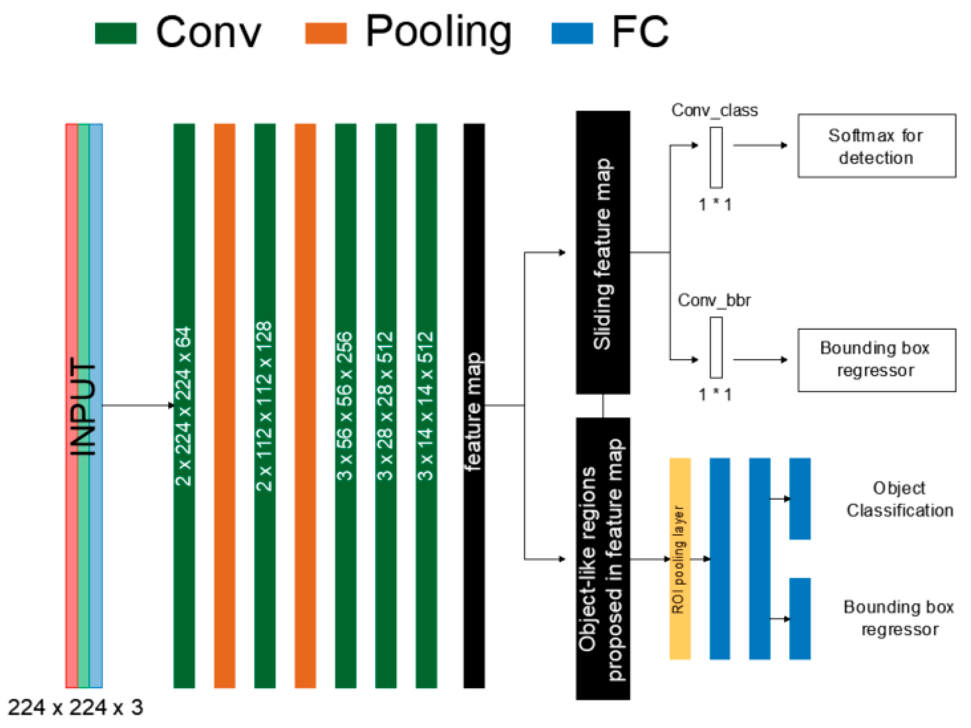
2.1. Faster R-CNN

The work of Faster R-CNN (Faster Region Convolution Neural Network) can be divided into two stages [15]. In the first stage, the input data are processed using the feature extractor and the VGG16 model [10]. The result of this process is a map of features that is used in the next stage. In this part, Faster R-CNN consists of two networks. The first is the Region Proposal Network (RPN), which is responsible for generating regions (called a region proposal), on the basis of which the second network performs structure detection. This is directed at those regions that most likely contain objects. As a result, the time needed to generate the proposed regions is reduced (Figure 1).

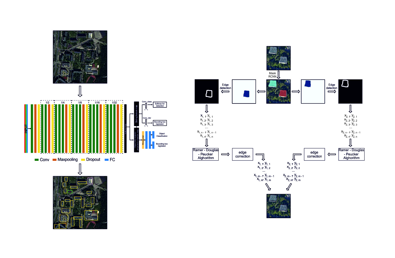
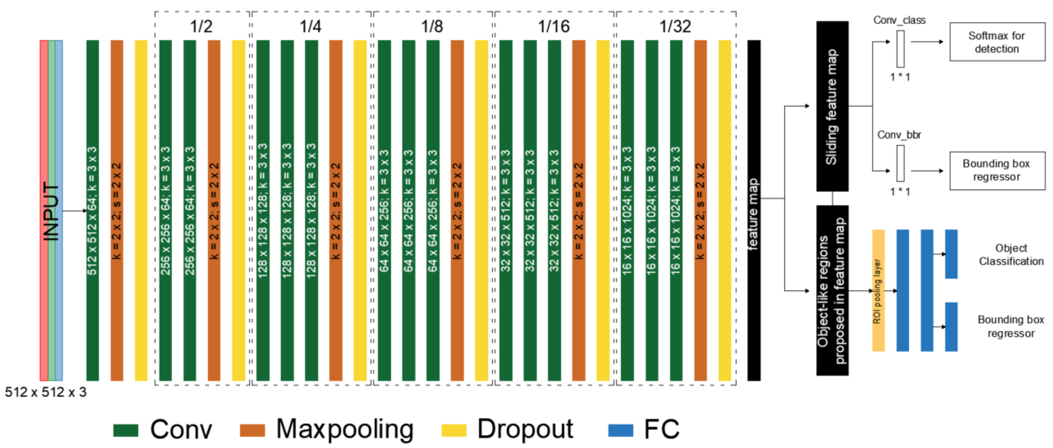
2.2. Our Method: Faster Edge Region CNN

FER-CNN (Figure 2) was used to train the network, in which our own convolutional network was used, generating a feature map. This network consists of six modules, followed by a Maxpooling and Dropout layer. In addition, the parametric PReLu [Parametric Rectified Linear Unit] activation function was used.

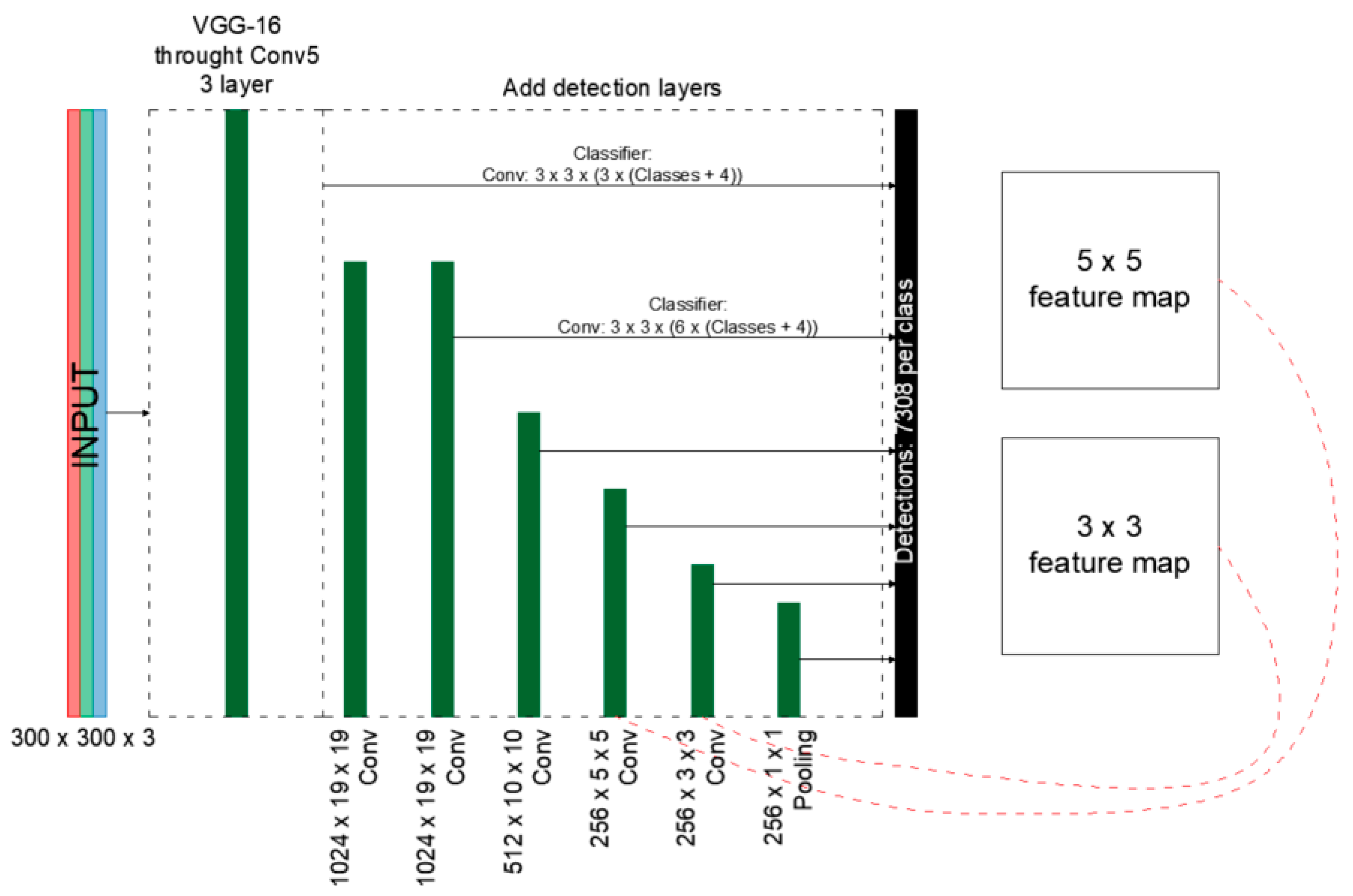
2.3. Single-Shot MultiBox Detector Network

The second stage of research on the impact of the optimization method on the detection and classification of structures was to train the model based on the Single-Shot MultiBox Detector (SSD) network [17]. This model was proposed by Christian Szegedy’s team in 2016 [11] to increase the efficiency and precision of structure detection. It is based on the VGG-16 architecture; however, the fully connected layers were replaced by additional convolution layers, enabling the detection of structures of different sizes and the gradual reduction of the output data size for subsequent layers (Figure 3).

2.4. Mask R-CNN

Mask R-CNN is a deep neural network designed for instance segmentation of a structure, which, unlike Faster R-CNN and SSD, not only provides information about the bounding box but also inlays a mask on the image similar in shape to the outline of the object [35]. This architecture differs significantly from the previously described methods, and it works in two stages: first, it generates suggestions for regions in which the structure may be located; next, it predicts the class of the object, corrects the coordinates of the bounding box and then creates a mask at the pixel level.

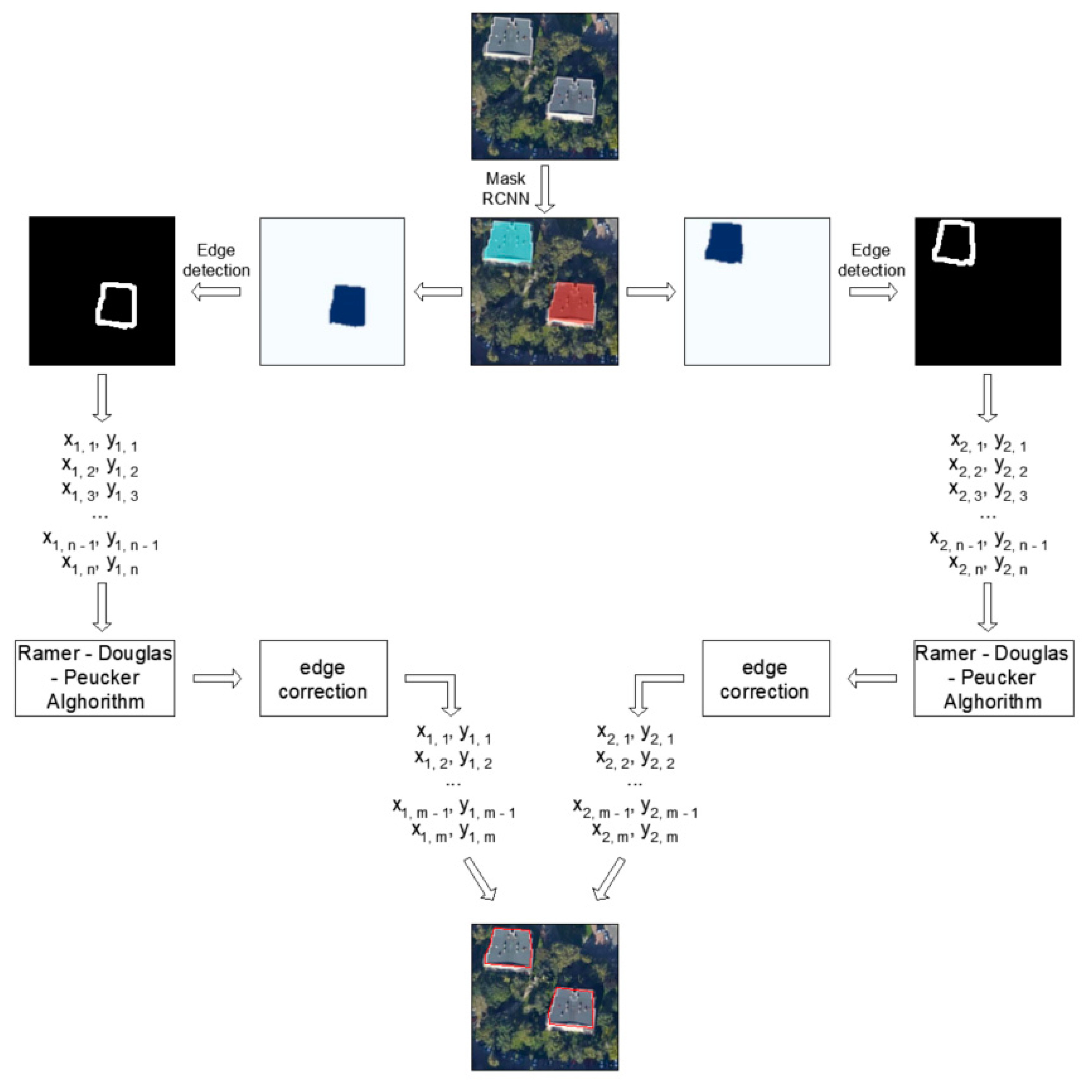
By using Mask R-CNN, it is possible to detect a structure in the image and obtain its approximate shape. The disadvantage of this action is that the building is represented with a mask, so the exact location of its edges and their coordinates are unknown. In order to solve this problem, we propose a method that makes it possible to detect buildings in a satellite image while maintaining its membership to one of the defined categories.

This algorithm displays structures belonging to one class in the image and then uses the Ramer–Douglas–Peucker algorithm [36] to minimize the number of points that create the building contour. This operation is performed for each of the seven classes, and the result of the algorithm is an image that shows the boundaries of buildings (while maintaining their classification) and a set of image coordinates of the structure. As a result, we obtain a building contour that consists of a smaller number of points (Figure 4).

2.5. Building Boundary Regularization Method

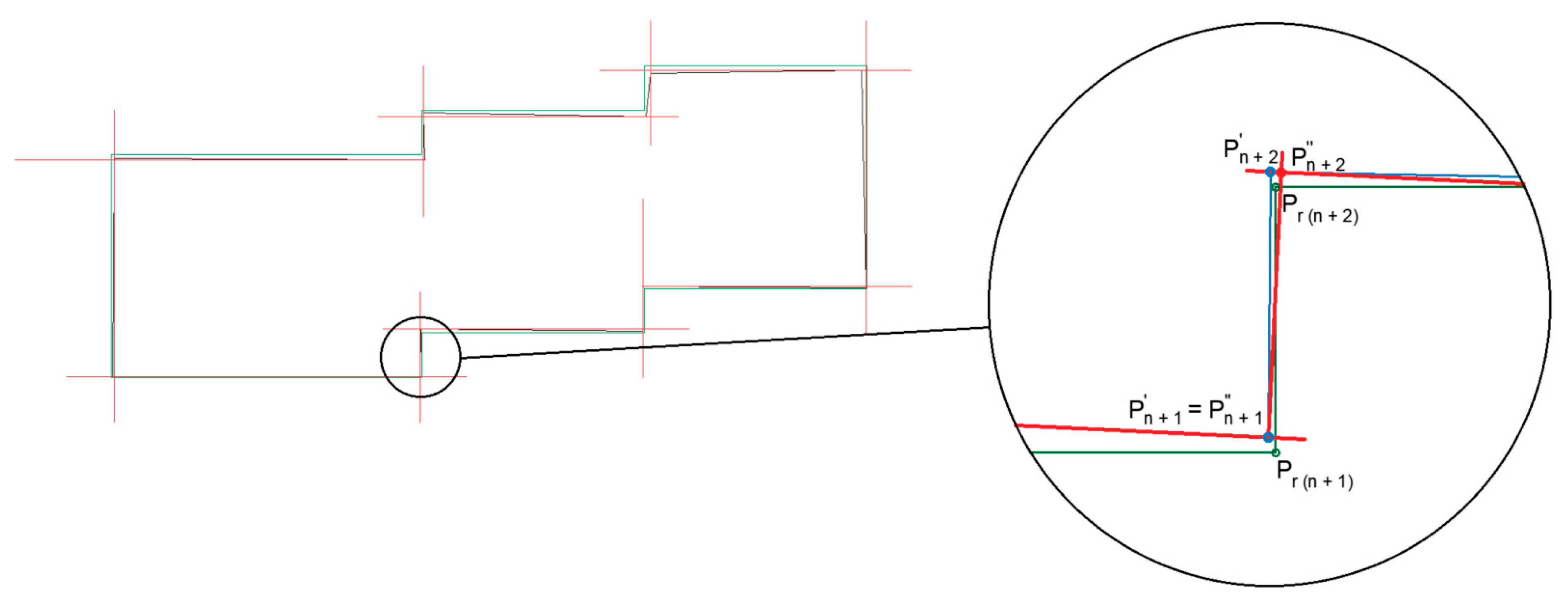
Given the nature of those structures, which are buildings, it can be seen that, in most cases, the adjacent walls of the building form a right angle with each other. On the basis of the above, we propose using the following algorithm to correct the detected edges while remembering that wall projections can also take other shapes (e.g., arches) (Figure 5).

The proposed method takes the first pair of points as the “base” edge P_nP_{n + 1} and then checks the angle that it creates with the next edge P_{n + 1}P_{n + 2}. If the sine value for this angle is in the range from 0.9925 to 1.0000, it is assumed that the angle error is less than 7° (condition I); it corrects this edge by leading a straight line perpendicular to the base edge that passes through the P_{n + 1} vertex, and then it projects the point P_{n + 2} onto this straight line to create point P’_{n + 2} (substitutes the coordinates of P_{n + 2} with P’_{n + 2}). As a result of this action, a new, corrected building edge is created with a beginning at P_{n + 1} and an end at P_{n + 2} (Figure 6).

Note that not all building edges intersect at right angles. Therefore, the condition in which the angle sine value is in the range from 0.1219 to 0.9925 (condition II) is considered. For this case, the length of the P_n+1P_n+2 segment is checked first, and if it is less than 5 pixels (in the case of a pixel size equal to 0.5 m, it is a length of less than 2.5 m), this indicates the “truncation” of a corner of the building. This phenomenon is very often found as a result of mask rounding on the corners. In such an instance, the program determines the corner of the building at the point of intersection of the lines that pass through the points P_n, P_n+1 and P_n+2, P_n+3 (it is first checked to determine whether these lines form an angle of 90° ± 7° with each other). If the length of the edge is longer than 5 pixels, the algorithm checks the next pair of edges; if it is less than five, it does not make corrections, but if it is at least 5, it approximates on the basis of these points (Equation (1)). This program also checks to determine whether there is a case in which all the angles of the figure will meet this condition. If so, then the program inscribes them in an ellipse (Equation (2)).

$$\phi \left(x\right)=a_0+a_{1}x+a_2{x}^2+\dots +a_m{x}^m={\displaystyle \sum }_{k=0}^m{a}_k{x}^k$$

(1)

$$\frac{x^2}{a^2}+\frac{y^2}{b^2}=1$$

(2)

Another condition that the program checks is the case in which the angle value is between 0.0000 and 0.1219 (condition III). If this condition is met, it checks the distance of the point P_n+1 from the line passing through the points P_n, P_n+2. If this distance is less than 5 pixels, the program removes the point P_n+1.

On the basis of the above-mentioned conditions, the algorithm checks all the edges of the figure, which is the first iteration (this algorithm performs three iterations because the differences in the shape of the building outline for a larger number is insignificant) (see Figure 7). In the case of a different spatial resolution, a correction of the distance between points and the straight line should be made.

3. Experiments and Results

This work explores the potential of convolution networks in the detection and classification of buildings in satellite images of urban and suburban areas.

All calculations included in this work were carried out using a PC with an Intel Core i5 CPU, NVIDIA 2070 RTX processor, 16 GB RAM memory and Ubuntu 16.04 operating system. In order to prepare images for network training, the Rasterio (v. 1.1.3), OpenCV (v. 4.1.0) and Numpy (v. 1.16.1) libraries were mainly used, while the Keras (v. 2.2.4) and TensorFlow (v. 1.13.1) libraries were used to implement neural network models.

First, a comparison was performed between Faster R-CNN, FER-CNN, and SSD in terms of their abilities to detect and classify structures, with a focus on the choice of network training hyperparameters because they play a very important role in successful and effective training and, therefore, also in the attainment of results with the best accuracy. The hyperparameters include the number of filters in the convolution layer and the activation function. The ReLU [Rectified Linear Unit] activation function was used in order to train Faster RCNN and SSD networks, while the parametric version of this function (PReLU) was used for Faster Edge Region CNN. Each model was trained for 200 epochs with a batch size of 2. For this purpose, a brief analysis of the impact of the optimization algorithm on the results was carried out. The aim of the optimization is to find the extremum of the set objective function, i.e., the optimal solutions to the problems posed. These algorithms differ from classic optimization methods. They work on the principle of indirect optimization of the performance of trained models by reducing the cost function, which will minimize the expected error, referred to as risk. The reason for using indirect optimization is that only a training database is available, which results in a lack of knowledge about the distribution of generated data. Overall, the optimizer’s task is to adjust the network with data from the loss function. The optimizer allows the best possible efficiency to be obtained for training data. Shortening the process of learning could be achieved by the appropriate choice of hyperparameter. Examples of such optimizers are Momentum, RMSProp and Adam.

Because there is a need to determine the exact location of buildings in the images, the Mask R-CNN performance was tested. With this mask, the buildings were detected by means of polygons with shapes similar to the buildings’ structures. By means of additional processing of the obtained results, the building’s shape was corrected using the RDP algorithm and the algorithm proposed in Section 2.4.

3.1. Experiment Data

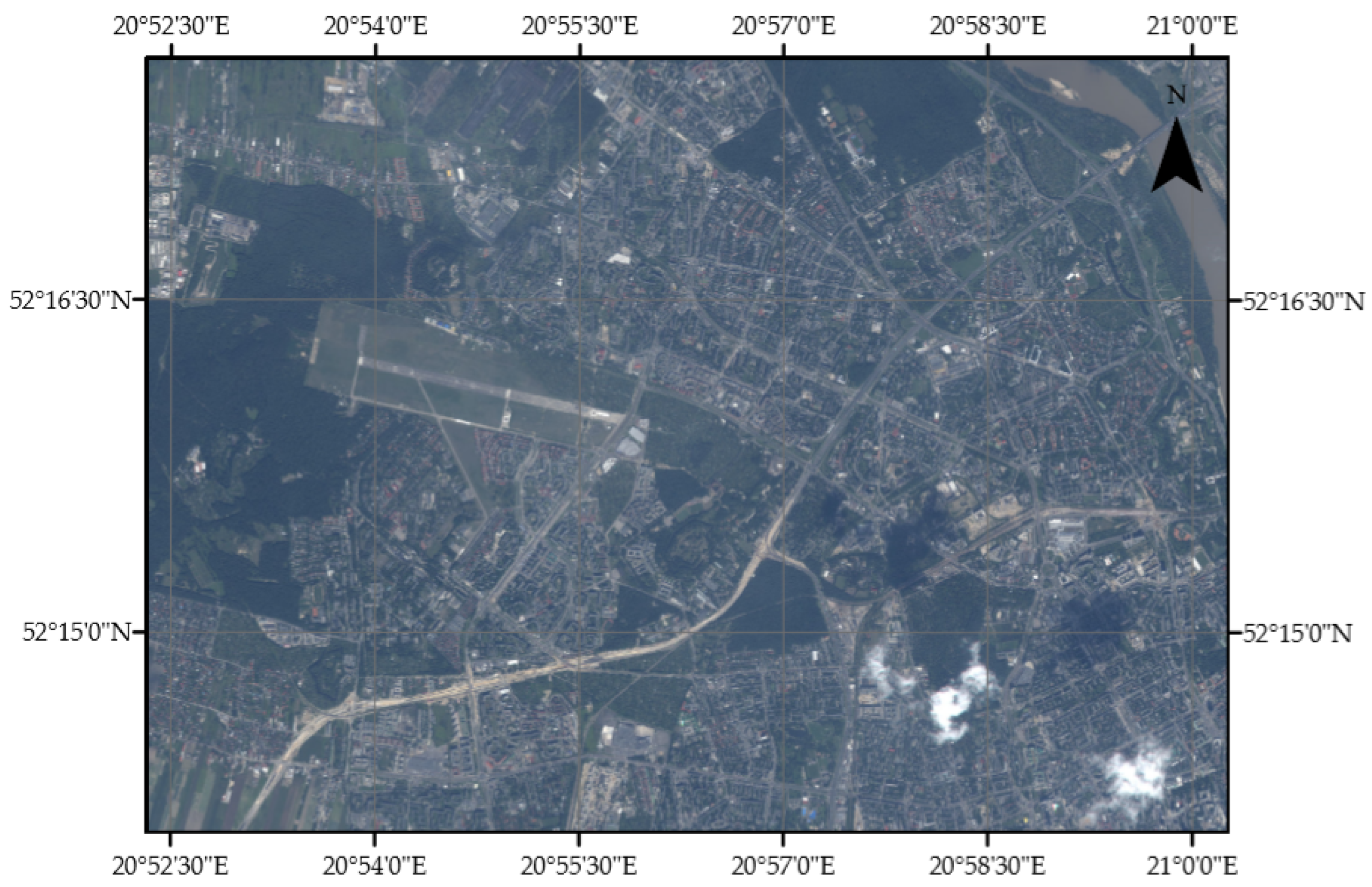
The database was created on the basis of satellite images that were obtained using WorldView-2 and Pléiades (see

Table 1. Technical characteristics of WorldView-2 and Pléiades satellites.

Satellite	Launch Date	Orbital Altitude [km]	Pan Resolution at Nadir [m]	MS Resolution at Nadir [m]	Swath Width [km]
WorldView-2	8 October 2009	770	0.46	1.8	16.5
Pléiades	2 December 2012	695	0.50	2.0	20

) satellites and show a fragment of the city of Warsaw and its periphery (Poland).

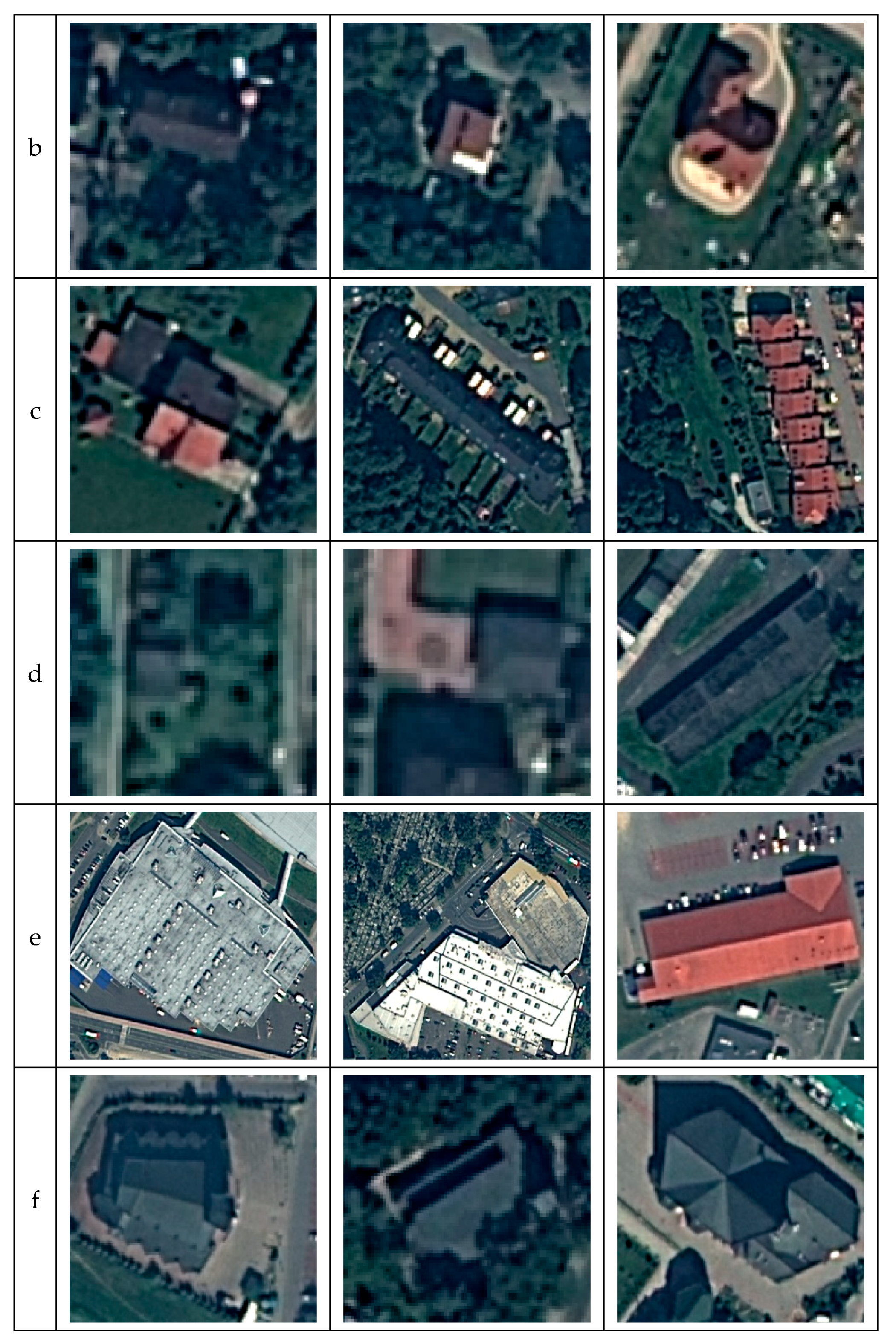
The studied area covers the western part of Warsaw and is located in a rectangle limited by the 20°52′19″ E, 21°00′07″ E meridians and the 52°14′05″ N, 52°17′58″ N latitudes (Figure 8) in the WGS-84 reference system in the UTM system. From this image, six areas with different urban characteristics are distinguished: (1) apartment blocks with garages, (2) a block of flats with small shops, (3) diversified cases with occlusion, (4) dense block buildings, (5) structures shaded by trees or images with low contrast between buildings and the surroundings and (6) dense single-family houses and terraced buildings.

Before performing operations on the image, in order to increase their resolution, pan sharpening was performed, which increased the resolution of the multispectral image to 0.5 m. These images were divided into smaller ones that measure 512 × 512. We used our own script for this, which divides the image into smaller parts with a vertical step of 250 and horizontal step of 350 pixels. As a result, a database was created consisting of 500 images with red, green, and blue channels and a spatial resolution of 0.5 m, which was divided into three sets of data: training (350 images), validation (75 images) and test (75 images).

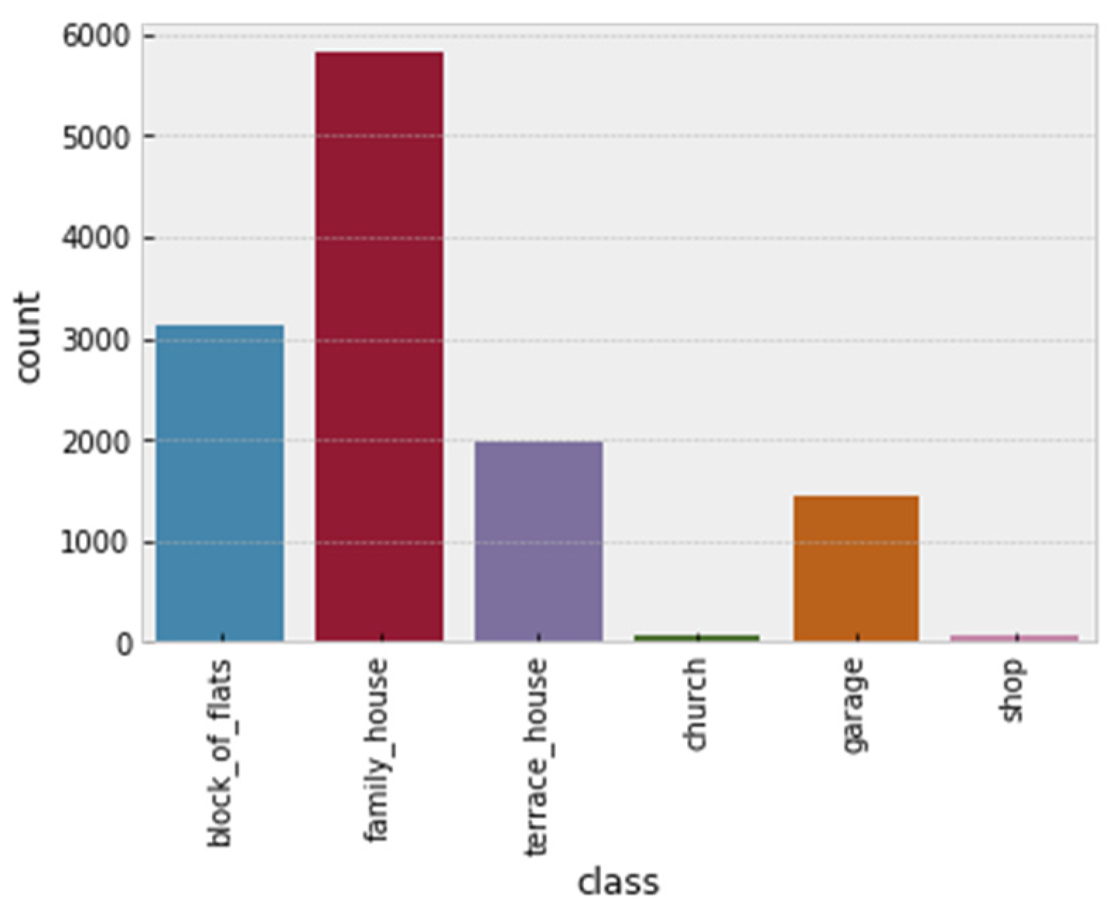
In the resulting database, about 12,500 buildings of various types were marked with LabelImg [37]. They were divided into six categories: shopping center, block of flats, church, terraced houses, single-family house and garage (see Figure 9).

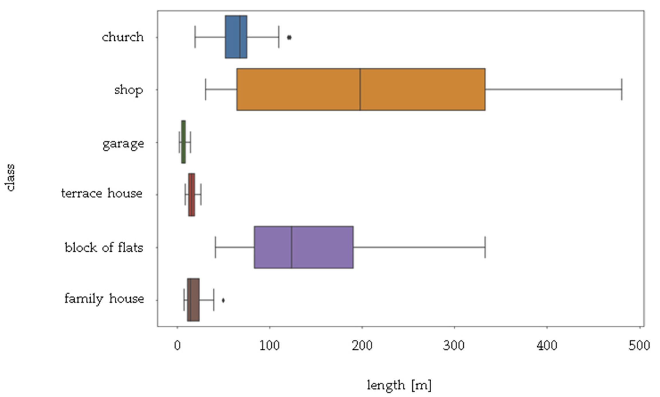
Selected types of objects differ from each other by many parameters, including size, height, shape and roof (along with the installations located on it). A crucial feature that allows buildings to be distinguished is their size, which is why Figure 10 shows the difference between the horizontal dimensions of sample buildings in each category. The largest building of the featured classes is the shopping center, while the smallest is the garage (see Figure 10).

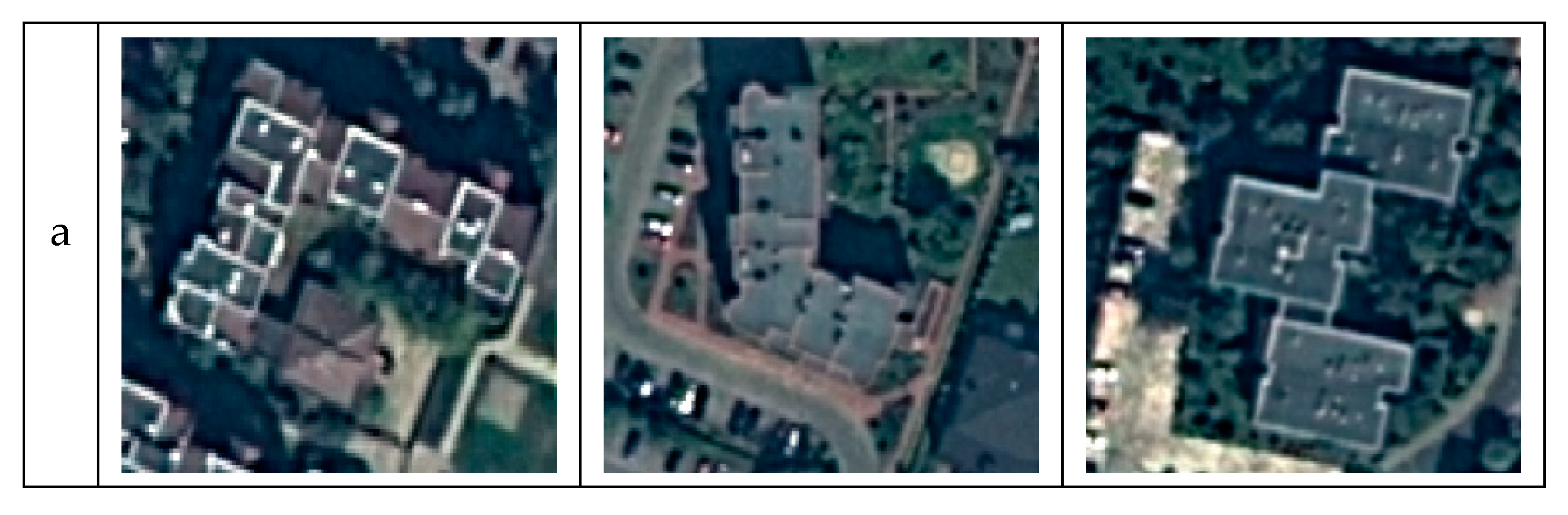
Architectural variability within specific classes is an additional difficulty in classification. This phenomenon is very clearly visible among single-family homes. These structures can have different dimensions, shape, number of floors, or even a different type of structure. In the case of terraced buildings (or garages), another difficulty is the occurrence of different values for the ratio of the length of the sides of the structure because it can consist of either three or ten segments (see Figure 11).

The number of image pixels also affects the classification of buildings. In the WorldView-2 images, a small single-family house with dimensions of 8 × 10 m is made up of about 320 pixels, which makes it possible to identify many elements on the surface of the roof (installations, chimneys) and to determine the type of roof. In the case of images with lower resolution, e.g., acquired using the Ikonos satellite (where the resolution of the images is 1 m), the same building will consist of about 80 pixels, which makes it impossible to identify the details of the roof, and so models trained on the basis of these data cannot cope with classification.

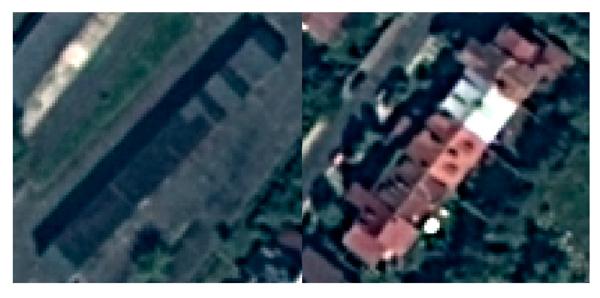
The similarity among classes is another problem. This phenomenon is visible in the case of terraced houses and garages. These buildings can be distinguished from each other by the details on their roofs. In the case of images with lower resolution (or quality), the differences between these categories are small, which is why their proper identification on the basis of their surroundings is possible (see Figure 12). Classical methods of building detection in satellite images are very time-consuming and do not allow for division by their destination. Although edge detection or segmentation techniques provide the possibility to detect buildings, they require particular parameter choices for each image. In our method, data preparation for the algorithm and training are the most time-consuming, and when using the network, achieving results depends on image import.

In addition, it should be noted that because of their diverse architecture, these types of structures are characterized highly variable shapes, and besides this, they are often accompanied by shadows, occlusion, noise, deformations, variable lighting or different resolutions (see

Table 2. Factors influencing the accuracy of building detection and classification.

Occlusion	Lighting
Background	Scale
Deformation	Type
Resolution variation	Shadows

). These factors have a significant impact on the algorithms’ performance, especially in urban areas, where building density is very high. In this case, an often-occurring phenomenon is the overlapping of building shadows on neighboring objects, or the “laying of buildings”, which can lead to the merging of many buildings into one.

When working with satellite imagery, these structures are identified only on the basis of roofs and the surroundings. In this case, one must pay attention to the heterogeneity of the roofs and the possibility of additional installations being present on them (which is possible, but not necessary).

3.2. Accuracy Assessment

To assess the accuracy of the detection and classification of structures, three parameters can be used: accuracy detection (AD) (Equation (3)), missing ratio (MR) (Equation (4)), and false-positive classification rate (FPCR) (Equation (5)).

$$AD=\frac{number of structures detected}{number of all structures}$$

(3)

$$MR=\frac{number of undetected structures}{number of all structures}$$

(4)

$$FPCR=\frac{number of incorrectly classified structures}{number of all classified structures detected}$$

(5)

3.3. Experimental Results

3.3.1. Results of Faster R-CNN

First, three Faster R-CNN networks were trained using three optimization methods: Adam, Momentum and RMSProp. The training process was carried out for a constant number of iterations.

The results of the optimization are presented in

Table 3. Detection of structures using the Faster R-CNN architecture.

Faster R-CNN
Adam	Momentum	RMSProp

. The table presents a record of structure detectability in images. This was used to check the correct operation of the models. The assessment was made using parameters that determine the quality of building detection and classification. Detailed assessment results are provided in the Appendix A.

Table A1. Summary of structure detection for Sets 1–6: Faster R-CNN architecture.

		Set 1			Set 2			Set 3			Set 4			Set 5			Set 6
		A	M	R	A	M	R	A	M	R	A	M	R	A	M	R	A	M	R
garage	W	4	4	6	1	0	0	0	0	0	0	0	0	1	0	0	0	0	0
	T	4	4	6	0	0	0	0	0	0	0	0	0	0	0	0	0	0	0
	F	0	0	0	1	0	0	0	0	0	0	0	0	1	0	0	0	0	0
	B	7	7	5	0	0	0	0	0	0	0	0	0	0	0	0	0	0	0
	S	11	11	11	0	0	0	0	0	0	0	0	0	0	0	0	0	0	0
terraced house	W	6	5	5	0	0	0	3	2	3	0	0	1	0	0	0	26	1	23
	T	5	3	3	0	0	0	2	2	2	0	0	0	0	0	0	25	1	22
	F	1	2	2	0	0	0	1	0	1	0	0	1	0	0	0	1	0	1
	B	5	7	7	0	0	0	1	1	1	0	0	0	0	0	0	11	35	14
	S	10	10	10	0	0	0	3	3	3	0	0	0	0	0	0	36	36	36
Single-family house	W	7	12	14	0	0	0	2	3	2	0	0	0	2	2	3	73	88	71
	T	4	6	6	0	0	0	1	1	1	0	0	0	0	0	0	60	59	59
	F	3	6	8	0	0	0	1	2	1	0	0	0	2	2	3	13	29	12
	B	3	2	2	0	0	0	0	0	0	0	0	0	0	0	0	4	5	5
	S	8	8	8	0	0	0	1	1	1	0	0	0	0	0	0	64	64	64
block of flats	W	21	24	23	19	19	21	7	4	7	36	33	34	16	15	16	0	0	0
	T	21	19	21	18	17	19	6	3	7	36	33	33	16	15	16	0	0	0
	F	0	5	2	1	2	2	1	1	0	0	0	1	0	0	0	0	0	0
	B	3	5	1	2	4	2	1	4	0	5	8	8	2	3	2	0	0	0
	S	24	24	24	21	21	21	7	7	7	41	41	41	18	18	18	0	0	0
church	W	0	0	0	0	0	0	1	1	1	0	0	0	0	0	0	0	0	0
	T	0	0	0	0	0	0	1	1	1	0	0	0	0	0	0	0	0	0
	F	0	0	0	0	0	0	0	0	0	0	0	0	0	0	0	0	0	0
	B	0	0	0	0	0	0	1	1	1	0	0	0	0	0	0	0	0	0
	S	0	0	0	0	0	0	2	2	2	0	0	0	0	0	0	0	0	0
Shopping center	W	0	0	0	1	1	1	1	1	1	1	0	0	1	2	1	0	0	0
	T	0	0	0	1	1	1	1	1	1	1	0	0	1	1	1	0	0	0
	F	0	0	0	0	0	0	0	0	0	0	0	0	0	0	0	0	0	0
	B	0	0	0	1	1	1	0	0	0	1	2	2	1	1	1	0	0	0
	S	0	0	0	2	2	2	1	1	1	2	2	2	2	2	2	0	0	0

W: detected objects; T: true objects; F: false objects; B: undetected objects; S: number of buildings on the image; A: Adam optimizer; M: Momentum; R: RMSProp optimizer.

,

Table A2. Summary of structure detection for Sets 1–6: FER-CNN architecture.

		Set 1			Set 2			Set 3			Set 4			Set 5			Set 6
		A	M	R	A	M	R	A	M	R	A	M	R	A	M	R	A	M	R
garage	W	5	7	8	1	0	0	0	0	0	0	0	0	2	0	0	0	0	0
	T	5	7	7	0	0	0	0	0	0	0	0	0	0	0	0	0	0	0
	F	0	0	0	1	0	0	0	0	0	0	0	0	0	0	0	0	0	0
	B	6	4	3	0	0	0	0	0	0	0	0	0	0	0	0	0	0	0
	S	11	11	11	0	0	0	0	0	0	0	0	0	0	0	0	0	0	0
terraced house	W	7	3	3	0	0	0	3	2	3	0	0	1	0	0	0	28	0	24
	T	6	2	3	0	0	0	2	2	2	0	0	0	0	0	0	27	0	23
	F	1	1	0	0	0	0	1	0	1	0	0	1	0	0	0	1	0	1
	B	0	0	0	0	0	0	1	1	1	0	0	0	0	0	0	9	36	13
	S	10	10	10	0	0	0	3	3	3	0	0	0	0	0	0	36	36	36
Single-family house	W	11	13	15	0	0	0	2	3	2	0	0	0	2	2	3	72	91	74
	T	5	6	7	0	0	0	1	1	1	0	0	0	0	0	0	62	63	63
	F	6	7	1	0	0	0	1	2	1	0	0	0	2	2	3	10	28	11
	B	1	0	0	0	0	0	0	0	0	0	0	0	0	0	0	2	1	1
	S	8	8	8	0	0	0	1	1	1	0	0	0	0	0	0	64	64	64
block of flats	W	23	24	24	22	18	21	7	4	7	38	36	35	16	15	16	0	0	0
	T	23	20	22	21	17	20	6	3	7	38	36	34	16	15	16	0	0	0
	F	0	4	2	1	1	1	1	1	0	0	0	1	0	0	0	0	0	0
	B	1	4	2	0	4	1	1	4	0	3	5	7	2	3	2	0	0	0
	S	24	24	24	21	21	21	7	7	7	41	41	41	18	18	18	0	0	0
church	W	0	0	0	0	0	0	1	1	1	0	0	0	0	0	0	0	0	0
	T	0	0	0	0	0	0	1	1	1	0	0	0	0	0	0	0	0	0
	F	0	0	0	0	0	0	0	0	0	0	0	0	0	0	0	0	0	0
	B	0	0	0	0	0	0	1	1	1	0	0	0	0	0	0	0	0	0
	S	0	0	0	0	0	0	2	2	2	0	0	0	0	0	0	0	0	0
Shopping center	W	0	0	0	1	1	1	1	1	1	1	0	0	1	2	1	0	0	0
	T	0	0	0	1	1	1	1	1	1	1	0	0	1	1	1	0	0	0
	F	0	0	0	0	0	0	0	0	0	0	0	0	0	0	0	0	0	0
	B	0	0	0	1	1	1	0	0	0	1	2	2	1	1	1	0	0	0
	S	0	0	0	2	2	2	1	1	1	2	2	2	2	2	2	0	0	0

W: detected objects; T: true objects; F: false objects; B: undetected objects; S: number of buildings on the image; A: Adam optimizer; M: Momentum; R: RMSProp optimizer.

and

Table A3. Summary of structure detection for sets 1-6: SSD architecture.

		Set 1			Set 2			Set 3			Set 4			Set 5			Set 6
		A	M	R	A	M	R	A	M	R	A	M	R	A	M	R	A	M	R
garage	W	1	0	0	0	0	0	0	0	0	0	0	0	0	0	0	0	0	0
	T	0	0	0	0	0	0	0	0	0	0	0	0	0	0	0	0	0	0
	F	1	0	0	0	0	0	0	0	0	0	0	0	0	0	0	0	0	0
	B	11	11	11	0	0	0	0	0	0	0	0	0	0	0	0	0	0	0
	S	11	11	11	0	0	0	0	0	0	0	0	0	0	0	0	0	0	0
terraced house	W	0	7	8	0	0	0	0	2	3	0	1	0	0	0	0	0	14	13
	T	0	6	6	0	0	0	0	1	2	0	0	0	0	0	0	0	10	13
	F	1	1	2	0	0	0	0	1	1	0	1	0	0	0	0	0	4	0
	B	10	4	4	0	0	0	3	2	1	0	0	0	0	0	0	36	26	23
	S	10	10	10	0	0	0	3	3	3	0	0	0	0	0	0	36	36	36
Single-family house	W	0	9	7	0	0	0	0	0	0	0	0	0	0	0	0	4	68	57
	T	0	5	4	0	0	0	0	0	0	0	0	0	0	0	0	0	53	49
	F	0	4	3	0	0	0	0	0	0	0	0	0	0	0	0	4	15	8
	B	8	3	4	0	0	0	1	1	1	0	0	0	0	0	0	64	11	15
	S	8	8	8	0	0	0	1	1	1	0	0	0	0	0	0	64	64	64
block of flats	W	4	22	21	4	18	21	2	7	7	2	29	32	1	11	13	0	0	0
	T	0	21	20	0	18	20	0	6	6	0	29	32	0	11	13	0	0	0
	F	4	1	1	4	0	1	0	1	1	2	0	0	0	0	0	0	0	0
	B	24	3	4	21	3	1	7	1	1	41	12	9	18	7	5	0	0	0
	S	24	24	24	21	21	21	7	7	7	41	41	41	18	18	18	0	0	0
church	W	0	0	0	0	0	0	0	1	1	0	0	0	0	0	0	0	0	0
	T	0	0	0	0	0	0	0	0	1	0	0	0	0	0	0	0	0	0
	F	0	0	0	0	0	0	0	0	0	0	0	0	0	0	0	0	0	0
	B	0	0	0	0	0	0	2	1	1	0	0	0	0	0	0	0	0	0
	S	0	0	0	0	0	0	2	2	2	0	0	0	0	0	0	0	0	0
Shopping center	W	0	0	0	0	3	0	1	1	1	0	0	0	1	1	1	0	1	0
	T	0	0	0	0	1	0	1	1	1	0	0	0	1	1	1	0	0	0
	F	0	0	0	0	2	0	0	0	0	0	0	0	0	0	0	0	1	0
	B	0	0	0	2	1	2	0	0	0	2	2	2	1	1	1	0	0	0
	S	0	0	0	2	2	2	1	1	1	2	2	2	2	2	2	0	0	0

W: detected objects; T: true objects; F: false objects; B: undetected objects; S: number of buildings on the image; A: Adam optimizer; M: Momentum; R: RMSProp optimizer.

(see Appendix A) compare five parameters that determine the correctness of the network operation: detected objects (W), true objects (T), false objects (F), undetected objects (B) and the number of buildings in the image (S). These parameters allow for an assessment of an algorithm’s results. The main parameters are detected objects, true objects and the number of buildings in the image. Their application shows that the Adam and RMSProp algorithms yield good results (see Table 3). The second of these methods achieves slightly better results for images 1 and 3, but the Adam algorithm is unrivaled compared with the others: in the case of visual analysis, it correctly determines the location of structures in the image.

The classification process of detected structures is also performed most accurately when using the Adam method. In addition, it can be seen that the most recognizable structures are the block of flats, while garages are the least recognizable.

FPCR: False-Positive Classification Rate

From the three parameters that define the accuracy of detection (

Table 4. Accuracy assessment of the model’s operation: Faster R-CNN.

		AD	MR	FPCR	Correctness of Class Detection
					G	T	F	B	CH	S
Set 1	A	0.72	0.34	0.12	0.36	0.60	0.63	0.88	-	-
	M	0.85	0.40	0.41	0.36	0.20	0.50	0.79	-	-
	R	0.91	0.28	0.33	0.55	0.30	0.50	0.88	-	-
Set 2	A	0.91	0.13	0.11	-	-	-	0.90	-	0.50
	M	0.87	0.22	0.11	-	-	-	0.90	-	0.50
	R	0.96	0.13	0.10	-	-	-	1.00	-	0.50
Set 3	A	0.88	0.19	0.27	-	0.67	1.00	0.86	0.50	1.00
	M	0.69	0.38	0.38	-	0.67	1.00	0.43	0.50	1.00
	R	0.88	0.13	0.17	-	0.67	1.00	1.00	0.50	1.00
Set 4	A	0.86	0.14	0.00	-	-	-	0.88	-	0.50
	M	0.77	0.23	0.00	-	-	-	0.80	-	1.00
	R	0.81	0.23	0.06	-	-	-	0.80	-	0.00
Set 5	A	1.00	0.15	0.18	-	-	-	0.89	-	0.50
	M	0.95	0.20	0.13	-	-	-	0.83	-	1.00
	R	1.00	0.15	0,18	-	-	-	0.89	-	0.50
Set 6	A	0.99	0.15	0.16	-	0.69	0.94	-	-	-
	M	0.89	0.40	0.48	-	0.03	0.92	-	-	-
	R	0.94	0.19	0.16	-	0.61	0.92	-	-	-

A: Adam optimizer; M: Momentum; R: RMSProp optimizer; AD: accuracy detection; MR: missing ratio; FPCR: false-positive classification rate; G: garage; T: terrace house; F: single-family house; B: block of flats; CH: church; S: shopping center.

), it can be seen that the Adam algorithm provides the best results in the second, fourth, fifth and sixth set, while RMSProp does better in other cases. In addition, the correctness of detecting individual building types was examined. The fewest errors in the classification of buildings occur when using the Adam algorithm. The exception is set 3, for which better results are obtained with the RMSProp algorithm.

3.3.2. Result of Our Method, FER-CNN

To be able to compare the results of these two networks, the same assumptions were made: the same image database and the same set of images for visual assessment were used, and the duration of both networks’ training was equal to 200,000 steps.

The results of the program operation, depending on the optimization used, are presented in the tables below (see

Table 5. Detection of structures using the Faster Edge Region Convolution Neural Network (FER-CNN) architecture.

FER-CNN
Adam	Momentum	RMSProp

and

Table 6. Accuracy assessment of the model’s operation: FER-CNN.

		AD	MR	FPCR	Correctness of Class Detection
					G	T	F	B	CH	S
Set 1	A	0.87	0.15	0.13	0.45	0.60	0.63	0.96	-	-
	M	0.89	0.15	0.23	0.64	0.20	0.75	0.83	-	-
	R	0.94	0.09	0.06	0.64	0.30	0.88	0.92	-	-
Set 2	A	1.04	0.04	0.09	-	-	-	1.00	-	0.50
	M	0.83	0.22	0.04	-	-	-	0.81	-	0.50
	R	0.96	0.09	0.04	-	-	-	0.95	-	0.50
Set 3	A	1.00	0.21	0.21	-	0.67	1.00	0.86	0.50	1.00
	M	0.79	0.43	0.21	-	0.67	1.00	0.43	0.50	1.00
	R	1.00	0.14	0.14	-	0.67	1.00	1.00	0.50	1.00
Set 4	A	0.91	0.09	0.00	-	-	-	0.93	-	0.50
	M	0.84	0.16	0.00	-	-	-	0.88	-	0.00
	R	0.84	0.21	0.05	-	-	-	0.83	-	0.00
Set 5	A	1.05	0.15	0.10	-	-	-	0.89	-	0.50
	M	0.95	0.20	0.15	-	-	-	0.83	-	0.50
	R	1.00	0.15	0.15	-	-	-	0.89	-	0.50
Set 6	A	1.00	0.11	0.11	-	0.75	0.97	-	-	-
	M	0.91	0.37	0.28	-	0.00	0.98	-	-	-
	R	0.98	0.14	0.12	-	0.64	0.98	-	-	-

A: Adam optimizer; M: Momentum; R: RMSProp optimizer; AD: accuracy detection; MR: missing ratio; FPCR: false-positive classification rate; G: garage; T: terrace house; F: single-family house; B: block of flats; CH: church; S: shopping center.

). Significant improvement is visible when fitting the structures into a bounding box, so they contain less shadowing of buildings (Table 5). In addition, as in the first case, the best results in the detection and classification of structures occur for the Adam and RMSProp optimizations.

FPCR: False-Positive Classification Rate

Owing to the modification of the VGG-16 network architecture, significant improvements in the results are noticeable. There is an increase in the accuracy detection parameter (more buildings were detected), and a significant reduction in classification error can be observed. The program operating in this network model classifies structures significantly better, especially those that are particularly vulnerable to errors due to the similarity between classes, e.g., the side-by-side character of the construction of garages (Set 1).

3.3.3. Result of Single-Shot MultiBox Detector (SSD)

In the case of SSD, much better results are achieved for the RMSProp and Momentum algorithms. After applying the accuracy rating parameters, it can be seen that the first one achieves better results. Image 1 is an exception, for which the Momentum model is characterized by a slightly higher detection of buildings (

Table 7. Detection of structures using the SSD architecture.

Single-Shot MultiBox Detector
Adam	Momentum	RMSProp

).

After using the SSD model, one can notice a much larger number of buildings that are not detected in the image than that in the case of Faster R-CNN, while the number of incorrectly classified structures decreases (

Table 8. Accuracy assessment of the model’s operation: SSD architecture.

		AD	MR	FPCR	Correctness of Class Detection
					G	T	F	B	CH	S
Set 1	A	0.09	1.00	0.11	0.00	0.00	0.00	0.00	-	-
	M	0.72	0.40	0.11	0.00	0.60	0.63	0.88	-	-
	R	0.68	0.43	0.11	0.00	0.60	0.50	0.83	-	-
Set 2	A	0.17	1.00	0.17	-	-	-	0.00	-	0.00
	M	0.91	0.17	0.09	-	-	-	0.86	-	0.50
	R	0.91	0.13	0.04	-	-	-	0.95	-	0.00
Set 3	A	0.21	0.93	0.00	-	0.00	0.00	0.00	0.00	1.00
	M	0.79	0.36	0.14	-	0.33	0.00	0.86	0.00	1.00
	R	0.86	0.29	0.14	-	0.67	0.00	0.86	0.50	1.00
Set 4	A	0.05	0.95	0.05	-	-	-	0.00	-	0.00
	M	0.70	0.28	0.02	-	-	-	0.71	-	0.00
	R	0.74	0.26	0.00	-	-	-	0.78	-	0.00
Set 5	A	0.10	0.95	0.00	-	-	-	0.00	-	0.50
	M	0.60	0.40	0.00	-	-	-	0.61	-	0.50
	R	0.65	0.25	0.00	-	-	-	0.72	-	0.00
Set 6	A	0.04	1.00	0.00	-	0.00	0.00	-	-	-
	M	0.83	0.37	0.20	-	0.28	0.83	-	-	-
	R	0.70	0.38	0.08	-	0.36	0.77	-	-	-

A: Adam optimizer; M: Momentum; R: RMSProp optimizer; AD: accuracy detection; MR: missing ratio; FPCR: false-positive classification rate; G: garage; T: terrace house; F: single-family house; B: block of flats; CH: church; S: shopping center.

). Thus, it can be concluded that the SSD model is more accurate in terms of classification, but less accurate for structure detection.

In the case of SSD architecture, the accuracy detection parameter significantly worsens (depending on the image; for the RMSProp algorithm, it ranges from 0.65 to 0.91), which is also true for the missing ratio (for the same optimization method, it ranges from 0.25 to 0.40). Because fewer buildings are detected, there is a slight improvement in the classification error parameter, whose maximum value is 0.20.

3.3.4. Google Earth Image Database

In order to check the correctness of our method, the additional database was prepared, which consist of photos fragments from Google Earth. These photos show cities of different size, density and type of buildings—among the selected cities are Koszalin, Żyrardów, Opole and Suwałki. A database consists of 500 images, of different resolutions (the smallest image has a resolution of 241 × 306 pixels, and the largest- 856 × 1144 pixels), which were divided into two sets of data: training (400 images) and test (100 images). These images mark over 2200 buildings, which, as in the previous database, were divided into six categories: shopping center, block of flats, church, terraced houses, single-family house and garage. As in previous part, the three networks were trained for each architecture (Faster R-CNN, FER-CNN, SSD), which are differ from each other by the optimization method. The results are presented in

Table 9. Detection of structures using the Faster R-CNN, FER-CNN, SSD architecture.

	Faster R-CNN	FER-CNN	SSD
Adam
Momentum
RMSProp
Adam
Momentum
RMSProp
Adam
Momentum
RMSProp

.

As in the previous case of the database, consisting of fragments of satellite photos from the WorldView-2 satellite, the most relevant results can be reached using the FER-CNN network-based algorithm with the Adam optimization method. This algorithm has a significantly higher object detection rate (AD = 92%), while maintaining over 95% of correctness of the buildings classification. Additionally, the FER-CNN network-based algorithm has much higher accuracy in the detection of small objects (e.g., garage), even when they are partly shaded. In case of the total shading of the object and a roof color only slightly contrasting with the surrounding area, this algorithm does not detect these objects, similar to SSD and Faster R-CNN network-based detectors.

3.3.5. Box Detection

When comparing the operation of the above methods for the detection and classification of buildings in satellite images, one can see a significant advantage of our proposed FER-CNN (

Table 10. Comparing the results for Faster R-CNN, FER-CNN and SSD.

		Faster R-CNN			Our FER-CNN			SSD
		AD	MR	FPCR	AD	MR	FPCR	AD	MR	FPCR
Set 1	A	0.72	0.34	0.12	0.87	0.15	0.13	0.09	1.00	0.11
	M	0.85	0.40	0.41	0.89	0.15	0.23	0.72	0.40	0.11
	R	0.91	0.28	0.33	0.94	0.09	0.06	0.68	0.43	0.11
Set 2	A	0.91	0.13	0.11	1.00	0.04	0.09	0.17	1.00	0.17
	M	0.87	0.22	0.11	0.83	0.22	0.04	0.91	0.17	0.09
	R	0.96	0.13	0.10	0.96	0.09	0.04	0.91	0.13	0.04
Set 3	A	0.88	0.19	0.27	1.00	0.21	0.21	0.21	0.93	0.00
	M	0.69	0.38	0.38	0.79	0.43	0.21	0.79	0.36	0.14
	R	0.88	0.13	0.17	1.00	0.14	0.14	0.86	0.29	0.14
Set 4	A	0.86	0.14	0.00	0.91	0.09	0.00	0.05	0.95	0.05
	M	0.77	0.23	0.00	0.84	0.16	0.00	0.70	0.28	0.02
	R	0.81	0.23	0.06	0.84	0.21	0.05	0.74	0.26	0.00
Set 5	A	1.00	0.15	0.18	1.00	0.15	0.10	0.10	0.95	0.00
	M	0.95	0.20	0.13	0.95	0.20	0.15	0.60	0.40	0.00
	R	1.00	0.15	0.18	1.00	0.15	0.15	0.65	0.25	0.00
Set 6	A	0.99	0.15	0.16	1.00	0.11	0.11	0.04	1.00	0.00
	M	0.89	0.40	0.48	0.91	0.37	0.28	0.83	0.37	0.20
	R	0.94	0.19	0.16	0.98	0.14	0.12	0.09	1.00	0.11

). An additional advantage of this network is better resistance to shadows, which is very common in satellite images of urban areas.

Analyzing the comparison in Table 9, it can be seen that, in many cases, the smallest classification error occurs in the case of SSD networks. On this basis, it can be concluded that algorithms working on the basis of this network detect fewer objects, but with a smaller classification error.

3.3.6. Results of Edge Detection Using Mask R-CNN and Ramer–Douglas–Peucker (RDP)

The algorithm based on Mask R-CNN allows for the detection and classification of a structure using only 200 images in the training base. In addition, in order to check the algorithm’s ability to detect garages and small halls in the pictures, a seventh category of buildings was added—halls. It works well with objects of various sizes and those with low visibility due to low contrast with the surroundings, as well as with objects that are obscured by shadows. Moreover, this algorithm works well when it detects small structures such as garages or garden sheds (assumed to be in the garage category), as well as slightly larger warehouses (shopping centers).

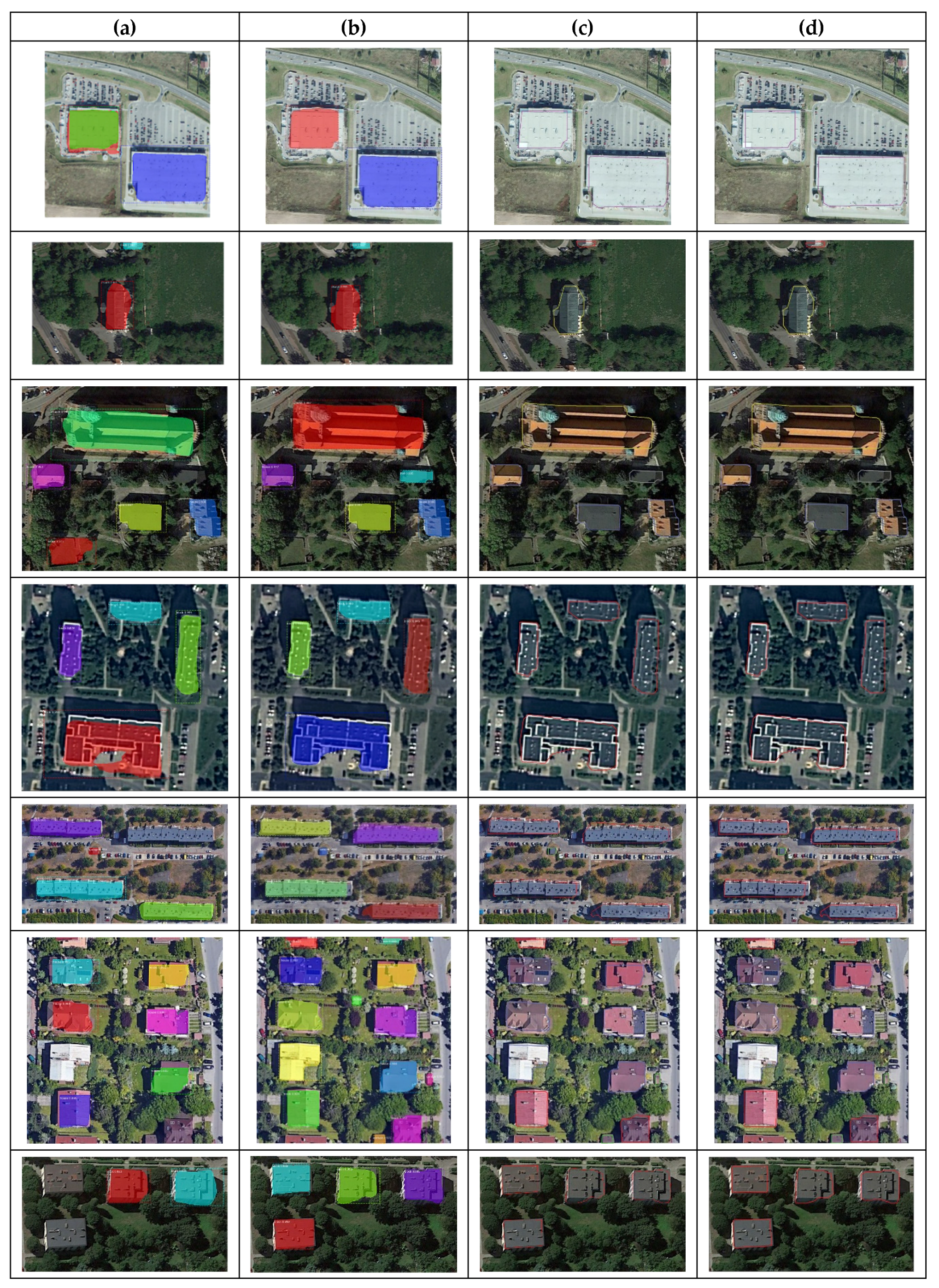
However, attention should be paid to the alignment of the mask generated by the algorithm with the actual contour of the building. For structures with simple shapes, this error is much smaller than it is for structures with complex shapes, e.g., churches and shopping centers (Figure 13a,b).

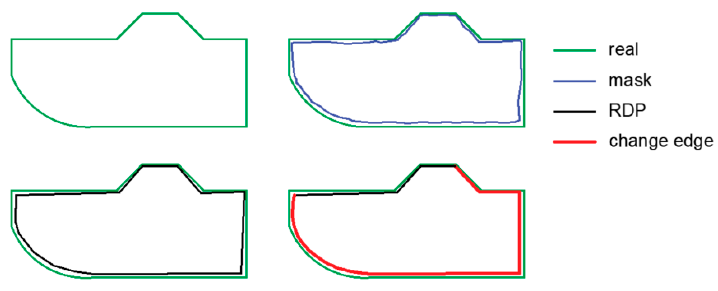
To obtain building outlines based on the generated masks, the RDP algorithm was used, followed by the proposed building boundary regularization method. Its application introduces a significant improvement in mapping the edges of buildings. In addition, as can be seen in Figure 13, distinguishing buildings with unusual architecture, such as churches or single-family terraced houses, is difficult, but our method can successfully recognize and locate them with faithful edge retention.

The algorithm we propose allows us to improve the edges generated by the RDP algorithm, but it depends on the quality of masks generated by Mask R-CNN. For Mask R-CNN, which was trained on the basis of a small database of 200 images, the method of building shape correction that we propose allows us to improve over 67% of angles on a right angle, as well as over 83% of edges. Due to these operations, the shape of the detected buildings is much closer to the real one. In the case of an increasing value of the parameter d_min (e.g., d_min = 10) and angle a₁ (e.g., a₁ = 12), we can increase the number of correctly made corrections to 89% for angles and to 93% for edges.

4. Discussion

This article presents the results of a comparative analysis of state-of-the-art CNN-based object detection method for determining and classifying buildings, along with a new method of improving building boundary regularization. All networks used in the study were trained on the basis of a dataset consisting of 500 images with red, green, and blue channels and a spatial resolution of 0.5 m. The best results were obtained with FER-CNN. The obtained test results prove the universality of the presented approach for high-resolution satellite imagery for the detection of buildings.

Comparing the results obtained by using Faster R-CNN, FER-CNN and SSD, it can be concluded that (1) models based on the Adam algorithm achieved good results only for Faster R-CNN, while they generated errors when used in SSD networks. (2) The modification of the VGG network resulted in the better detection of structures in the image, and it was more resistant to shadows. (3) The time required to train an SSD network was approximately three times longer than that for Faster R-CNN. (4) The SSD-based model did not detect buildings that had low contrast with the surroundings, but it generated fewer errors when classifying objects. (5) The size of the files needed to run Faster R-CNN was about five times larger than that for an SSD network.

On the basis of the comparative analyses performed, the effectiveness of our method was 97.5%; however, there is a significant difference between classes. In most cases, buildings that represent categories differ significantly, including in size and appearance (e.g., garages and shopping centers). In addition, it should be kept in mind that these networks mainly make mistakes when classifying the above objects. The proposed network is most often wrong in the classification of garages (especially those in terraced houses), where the detection accuracy error is 37% and the error of classification is only 6%. Therefore, before using the presented networks for utility purposes, it is necessary to improve their algorithms in this area.

Comparing our method with classic techniques that allow for the detection of buildings, the time needed to detect the defined categories of buildings is significantly reduced. In addition, this approach does not require the selection of individual parameters for each image.

In relation to other similar studies using the Faster R-CNN model based on the ResNet101 network, researchers obtained a classification accuracy of 99% with 2000 epochs, whereas building extraction using support vector machine achieved 88.3% [38]. WorldView-2 images were also part of our test material. Tests performed on these data also confirmed our conclusions that convolutional neural networks better extract features and detect structures in high-resolution images. The training time and prediction time of our algorithm is not much longer than Faster R-CNN, which is due to the higher value of the input resolution parameter (

Table 11. Comparing the training/prediction time for Faster R-CNN, FER-CNN and SSD.

	Input Resolution	Training Time	Prediction Time
Faster R-CNN	224 × 224	15 h	0.8 s
SSD	300 × 300	35 h	0.9 s
FER-CNN	512 × 512	19 h	1.0 s

). Other studies related to building detection have used the architecture of Res-U-N and Guided Filtering. An accuracy of 97% was achieved but without faithful reproduction of edges [21]. Other research results obtained by [39] showed that the use of an artificial neural network could produce an accuracy of 91.7%.

From our research results and the analysis of the data contained in Table 10, it can be seen that our method, compared with the others investigated, makes it possible to increase the number of detected and classified buildings in fragments of satellite images. In addition, the correctness of detecting buildings using bounding boxes significantly increases. However, we believe that these results can be improved by:

• Increasing the training base by adding images of other types of areas and buildings, paying particular attention to increasing the number of images of garages, shopping centers and churches;
• Increasing the number of iterations during network training;
• Further modifying Faster R-CNN.

In the second part of the research, buildings were detected using Mask R-CNN, and then the building boundary regularization process was performed. Our proposed method significantly improved the shape of the detected boundaries. However, a certain limitation of our method (as can be seen in Figure 13) is that the identified edges deviate slightly from the actual shape of the building. The reason for this phenomenon is the fact that completely covering a structure with a mask is a significant problem. The result of this may be too small a database or too few iterations made during network training. Apart from this disadvantage, the network detects and classifies structures very well, even those with a small surface area, although it must be taken into consideration that it sometimes fails to detect small structures, which do not have sufficient contrast with their surroundings.

5. Conclusions

In this work, the capabilities of neural networks in the detection and classification of buildings located in satellite images were examined. In the first stage of research, three network models were examined: Faster R–CNN, FER-CNN and SSD; additionally, the optimization method was taken into account. For the first of these architectures, the model using the Adam algorithm achieved the best results (it gave slightly better results than the Momentum algorithm). After performing the modification of the VGG network, a significant increase in the correctness of detecting buildings in images was noted, especially for the Adam algorithm, although the RMSProp algorithm also performed very well. In the case of the SSD-based model, the best results were obtained by using the RMSProp algorithm, while the worst performance was found in the Adam algorithm.

In the second stage of this work, the capabilities of the algorithm based on Mask R-CNN for the detection and classification of objects were investigated. Then, because of the irregular shape of the training polygons, a method was proposed that allowed us to obtain an image with the edges of classified buildings marked on it.

This algorithm coped well with the detection and classification of structures from satellite imagery; however, the generated edges were slightly different from the actual shape of the building, especially in the case of buildings with a complex structure, e.g., churches. The application of the method, which performs a correction of the edges of buildings, significantly improved the rendition of their actual shapes. However, attention should be paid to the size of the database on the basis of which the Mask R-CNN model was trained: in the first case, it contained 100 images, and in the second, it contained 200 images. This shows how great the possibilities are of the application of neural networks, even in the case of such a small amount of data.

From the above, it can also be stated that building extraction is still an important and current research topic and requires further experiments. In future work, we will focus on constructing a network for more reliable building classification, improving model performance for accurate edge extraction and developing a new model for using relationships between specific groups of buildings. In addition, we plan to design and train a neural network to detect small buildings and buildings with irregular shapes that are partially obscured by shadows or other occlusions. In addition, we plan to increase the efficiency of the proposed method and increase its automation.