Continuous Daily Evapotranspiration with Optical Spaceborne Observations at Sub-Kilometre Spatial Resolution

Abstract

Evapotranspiration (ET) is a key parameter in the description of the energy and water fluxes over land. Continuous and spatially detailed ET simulations are thus required for a number of scientific and management-related purposes. These conditions are determined by the modelling approach and the composition of the forcing dataset. This study aimed at simulating daily ET in a diversity of climate and land cover conditions at a spatial resolution of ∼1 km and higher. The modelling approach was based on the algorithm driving the ET product developed and set in operations in the framework of the Satellite Application Facility on Land Surface Analysis programme (LSA-SAF). The implemented algorithm allowed the ingestion of biophysical parameters derived from SPOT-V and PROBA-V observations developed by the Copernicus Global Land Programme, as well as other model parameters at a similar spatial resolution. The model was tested at an ∼1 km spatial resolution in over 40 sites located in different climate and land cover contexts. The implementation at ∼300 m was tested in the upper Biebrza basin, in Poland. The simulations correlated well with the validation dataset (r2 > 0.75 in 80% of sites) and exhibited root mean squared values lower than 1 mm/day in 80% of the cases. The results also pointed to the need for refining the accuracy of soil moisture data sources, especially in dry areas. The results showed the ability of the modelling approach and the SPOT-V/PROBA-V missions to support the generation of long ET time series. They also opened the gate to incorporate Sentinel-3 in ET continuous modelling.

1. Introduction

The timing and magnitude of energy and water fluxes at the Earth’s surface result from the interplay of a number of processes and conditions in the soil-plant-atmosphere continuum. The accurate description of those processes is a major concern towards understanding the mechanisms and drivers of terrestrial ecosystems.

The release of water vapour from the Earth’s surface into the atmosphere is called evapotranspiration (ET). ET comprises the volume of water evaporated from water bodies and reservoirs, the upper layers of the soil and intercepted water in different layers of the vegetation canopy, as well as the water transpired by photosynthetic organisms. Needless to say, the accurate and timely estimation of this component of the water balance is relevant in a large number of domains like agriculture monitoring and yield prediction [1], drought assessment [2,3,4], water catchments’ management [5,6], urban planning [7,8], etc.

ET plays a major role in the global climatic system as it is a key component of both the carbon and water cycle [9]. The heating effect of solar energy on Earth is tightly connected to ET as a substantial fraction of the solar radiation triggers the evaporative process (latent heat flux). The resulting ET rates also depend on local conditions (like water vapour demand, soil moisture, land cover, etc.).

The increasing interest in understanding and estimating ET at different spatial and temporal resolutions and in a continuous way has driven the development of algorithms and the search for optimal ways of exploiting available datasets to force those models. In this respect, a great deal of the developments and data exploration efforts are related to the use of spaceborne data in ET models [10] as the only means to visit every point on Earth on a regular basis virtually. These developments have been boosted in the last few years by the launch of satellite missions offering increased sampling frequency, spatial detail and timely availability in the generated datasets. More spatial detail in the observations implies better accounting for landscape heterogeneity, and a higher frequency of observations aids the construction of continuous time series of relevant land surface parameters.

This study aimed to generate continuous series of daily ET at an ∼1 km spatial resolution or higher in different ecosystems across the globe by combining remote sensing (RS) data, meteorological data and land cover-related parameters in a surface energy balance setting. Much attention was paid to the notion of continuity whereby: (a) daily ET series should cover several years and; (b) the number of missing values should be reduced to a minimum. These features rely on the availability of long and consistent time series of the model forcing variables and on algorithm-related characteristics coping with non-ideal conditions for RS observations; e.g., clouds.

As for continuity in RS data, the compatibility between the SPOT-Végétation (S-Vgt) and the PROBA-V mission offers interesting opportunities. The S-Vgt mission provided a wealth of spaceborne observations in the course of its operational life—between 1998 and 2014—at an ∼1 km spatial resolution. An important criterion in the design of the PROBA-V mission—operational since 2013—was the continuity of the S-Vgt observations and products. This aspect has been already explored and exploited in several studies [11,12,13]. In addition, the PROBA-V mission conducts observations with enhanced spatial detail (∼300 m and ∼100 m) while having equivalent radiometric characteristics across the three spatial resolutions.

The ET model in this study was based on the algorithm driving the operational ET product developed in the framework of the Land Surface Analysis Satellite Application Facility (LSA-SAF) [14,15,16]. The LSA-SAF ET algorithm has been in operation for about 10 years now and has proven its robustness in a number of applications [6,17,18,19,20] and the ability to operate in all-weather conditions [21].

This article presents an implementation of the principles at the basis of the LSA-SAF ET algorithm at an ∼1 km spatial resolution in various locations representing different ecosystems around the globe where in situ measured validation data were available. The study also includes ET simulations over a particular region in northern Poland where the spatial grid of PROBA-V 300 m products was the target spatial resolution. Finally, the study concludes with some considerations towards the opportunities given by Sentinel-3 to be ingested in the ET algorithm after the operational period of PROBA-V.

2. Materials and Methods

2.1. The ET Algorithm

The fundamentals of the algorithm can be expressed with the well known Equations (1) and (2) of the surface energy balance.

$$R_{net}=LE+H+G$$

(1)

$$R_{net}=(1-\alpha )S\downarrow +\epsilon (L\downarrow -\sigma T_{sk}^4)$$

(2)

where: $R_{net}$: net radiation; $LE$: latent heat flux; H: sensible heat flux; G ground heat flux; $\alpha$: albedo; $S\downarrow$ and $L\downarrow$: downwelling short and long wave solar radiation; $\epsilon$: emissivity; $\sigma$: the Stefan–Boltzmann constant; $T_{sk}$: skin temperature.

Various ET algorithms depart from these basic expressions, but differ in the approach followed to estimate the components, as well as in the forcing and the discretization of the temporal and spatial domains. The methods applied in this study followed greatly the algorithm powering the ET operational product designed in the framework of EUMETSAT’s programme Land Surface Analysis Satellite Application Facility (LSA-SAF) [14]. Thorough descriptions of this algorithm can be found in Ghilain et al. [15] and Ghilain et al. [16] and in the documentation of the LSA-SAF ET product (http://lsa-saf.eumetsat.int). The general lines of the procedure of ET estimation are described in the pseudocode presented in Figure 1.

The procedure indicated in Figure 1 was implemented at a time step of 30 min. The half-hourly estimates were then aggregated to obtain the target product: daily ET. The basic spatial unit was a cell c belonging to a gridded representation of the area of interest.

The procedure was fed by a series of variables and parameters containing information on incoming solar radiation and energy reflected by the surface ($S\downarrow$, $L\downarrow$, $\epsilon$, $\alpha$), vegetation type and dynamics (grouped as $veg$), soil moisture ($SM$), meteorological conditions (various variables grouped under $weather$) and the land cover classes ($lcover$) and their occupation fraction ($\zeta$) in each cell.

One cell may contain up to 4 tiles t, which corresponded to homogeneous land cover types. The computation of the energy balance was performed at the tile level. It occurred in an iterative way whereby the difference between $R_{net}$ and the aggregated energy fluxes was not allowed to exceed a threshold of 0.1; i.e., the energy balance closure was ensured. The occupation fraction of each tile $\zeta$ was then used to weigh the contribution of each tile to the ET cell value. The estimation of $LE$ and H was preceded by the computation of the response of vegetation to environmental determinants (canopy resistance) and the aerodynamic resistance. The former was driven by vegetation-related parameters ($veg$), soil moisture ($SM$) and the atmospheric water pressure deficit, which is related to the meteorological conditions ($weather$). The latter was determined by the atmosphere stability, derived from $weather$ and $lcover$. The soil heat flux (G) was computed as a function of $R_{net}$ and $veg$.

This algorithm was designed such that the temporal resolution of the forcing would account for the variability in major drivers of ET throughout the day; notably, solar radiation and meteorological conditions. It is noteworthy to point out that this algorithm computes the $T_{sk}$ term of Equation (2) in an iterative way. An alternative approach would be to retrieve land surface temperature (LST) from spaceborne data sources. Such an approach, however, would entail disadvantages related to the dependence of LST observations on cloudiness; it would then produce many gaps in the sub-daily ET estimates. The iterative estimation of $T_{sk}$ in an energy balance setting has proven effective to generate estimates equivalent to RS LST [21].

2.2. Study Sites

The set of study sites encompassed a large range of conditions in terms of climate and vegetation cover. The sites were selected such that in situ measured validation data were available; specifically, energy fluxes measured at eddy covariance (EC) towers. Most of the simulations were done on sites belonging to the FLUXNET network [22]. The FLUXNET data used in this study followed the guidelines of the CC-BY-4.0 data usage license (Attribution 4.0 International (CC BY 4.0); https://creativecommons.org/licenses/by/4.0/). The location of the study sites is shown in the map in Figure 2, which also shows the distribution of the Köppen–Geiger climatic classes as obtained by Beck et al. [23]. More details on these sites are shown in

Table 1. Acronym, name, simulated period, location and Köppen–Geiger climatic class of the FLUXNET sites where ET simulations were performed. The studied sites are grouped by plant functional type where CRO = cropland, DBF = deciduous broadleaf forest, EBF = evergreen broadleaf forest, ENF = evergreen needleleaf forest, GRA = grassland, MF = mixed forest, OSH = open shrubland, SAV = savanna, WET = wetland, WSA = woody savanna.

Site Acronym	Site Name	Country	Start Year	End Year	Longitude	Latitude	Climate Class
CRO
BE-Lon	Lonzee	Belgium	2004	2013	50.5516	4.7462	Cfb
DE-Kli	Klingenberg	Germany	2004	2013	50.8931	13.5224	Dfb
DE-RuS	Selhausen Juelich	Germany	2011	2013	50.8659	6.4471	Cfb
DE-Seh	Selhausen	Germany	2007	2010	50.8706	6.4496	Cfb
US-ARM	ARMSouthern Great Plains site-Lamont	United States	2003	2012	36.6058	−97.4888	Cfa
DBF
FR-Fon	Fontainebleau-Barbeau	France	2005	2013	48.47636	2.7801	Cfb
JP-MBF	Moshiri Birch Forest Site	Japan	2003	2005	44.3869	142.3186	Dfb
PA-SPn	Sardinilla Plantation	Panama	2007	2009	9.31814	−79.6346	Am
EBF
CN-Din	Dinghushan	China	2003	2005	23.1733	112.5361	Cwa
FR-Pue	Puechabon	France	2000	2013	43.7413	3.5957	Csa
GF-Guy	Guyaflux (French Guiana)	French Guyana	2004	2013	5.2788	−52.9249	Am
GH-Ank	Ankasa	Ghana	2011	2013	5.2685	−2.6942	Am
MY-PSO	Pasoh Forest Reserve (PSO)	Malaysia	2003	2009	2.9730	102.3062	Af
ENF
AR-Vir	Virasoro	Argentina	2009	2012	−28.2395	−56.1886	Cfa
CA-SF2	Saskatchewan	Canada	2001	2005	54.2539	−105.8775	Dfc
DE-Obe	Oberbärenburg	Germany	2008	2013	50.7867	13.7213	Dfb
DE-Tha	Tharandt	Germany	1999	2013	50.9626	13.5651	Dfb
FI-Hyy	Hyytiala	Finland	1999	2013	61.8474	24.2948	Dfc
FI-Let	Lettosuo	Finland	2009	2012	60.6418	23.9595	Dfc
NL-Loo	Loobos	The Netherlands	1996	2013	52.1666	5.7436	Cfb
RU-Fyo	Fyodorovskoye	Russia	1999	2013	56.4615	32.9221	Dfb
US-Me6	Metolius Young Pine Burn	United States	2010	2013	44.3233	−121.6078	Dsb
GRA
AU-DaP	Daly River Savanna	Australia	2007	2013	−14.0633	131.3181	Aw
AU-Stp	Sturt Plains	Australia	2008	2013	−17.1507	133.3502	BSh
US-SRG	Santa Rita Grassland	United States	2008	2013	31.7894	−110.8277	BSh
MF
BE-Bra	Brasschaat	Belgium	1999	2013	51.3076	4.5198	Cfb
BE-Vie	Vielsalm	Belgium	1999	2013	50.3049	5.9981	Dfb
CA-Gro	Ontario-Groundhog River, Boreal Mixed Wood Forest	Canada	2003	2013	48.2167	−82.1556	Dfb
CH-Lae	Laegern	Switzerland	2004	2013	47.4783	8.3644	Dfb
JP-SMF	Seto Mixed Forest Site	Japan	2002	2006	35.2617	137.0788	Cfa
US-SRC	Santa Rita Creosote	United States	2008	2013	31.9083	−110.8395	BSh
OSH
CA-NS6	UCI-1989 burn site	Canada	2001	2005	55.9167	−98.9644	Dfc
CA-SF3	Saskatchewan	Canada	2001	2006	54.0916	−106.0053	Dfc
US-Sta	Saratoga	United States	2005	2009	41.3966	−106.8024	BSk
SAV
AU-ASM	Alice Springs	Australia	2010	2013	−22.2830	133.2490	BWh
AU-DaS	Daly River Cleared	Australia	2008	2013	−14.1593	131.3881	Aw
AU-Dry	Dry River	Australia	2008	2013	−15.2588	132.3706	Aw
CG-Tch	Tchizalamou	Congo	2006	2009	−4.2892	11.6564	Aw
SD-Dem	Demokeya	Sweden	2005	2009	13.2829	30.4783	BWh
WET
DE-Spw	Spreewald	Germany	2010	2013	51.8922	14.0337	Dfb
RU-Che	Cherski	Russia	2002	2005	68.6130	161.3414	Dsc
WSA
AU-Ade	Adelaide River	Australia	2007	2009	−13.0769	131.1178	Aw
AU-How	Howard Springs	Australia	2001	2013	−12.4943	131.1523	Aw
US-SRM	Santa Rita Mesquite	United States	2004	2013	31.8214	−110.8661	BSh

.

The simulations on the sites listed in Table 1 were performed at a spatial resolution of 1 km (details on the forcing variables are given in further sections of this article). In addition to that, the algorithm was implemented at a 300 m resolution across the upper part of the Biebrza basin in Poland. The Biebrza basin is one of the largest and most valued protected areas in Europe. By virtue of its ecological value, it is listed in the Natura2000 network (https://ec.europa.eu/environment/nature/natura2000/) and belongs to RAMSAR convention for wetlands (https://www.ramsar.org).

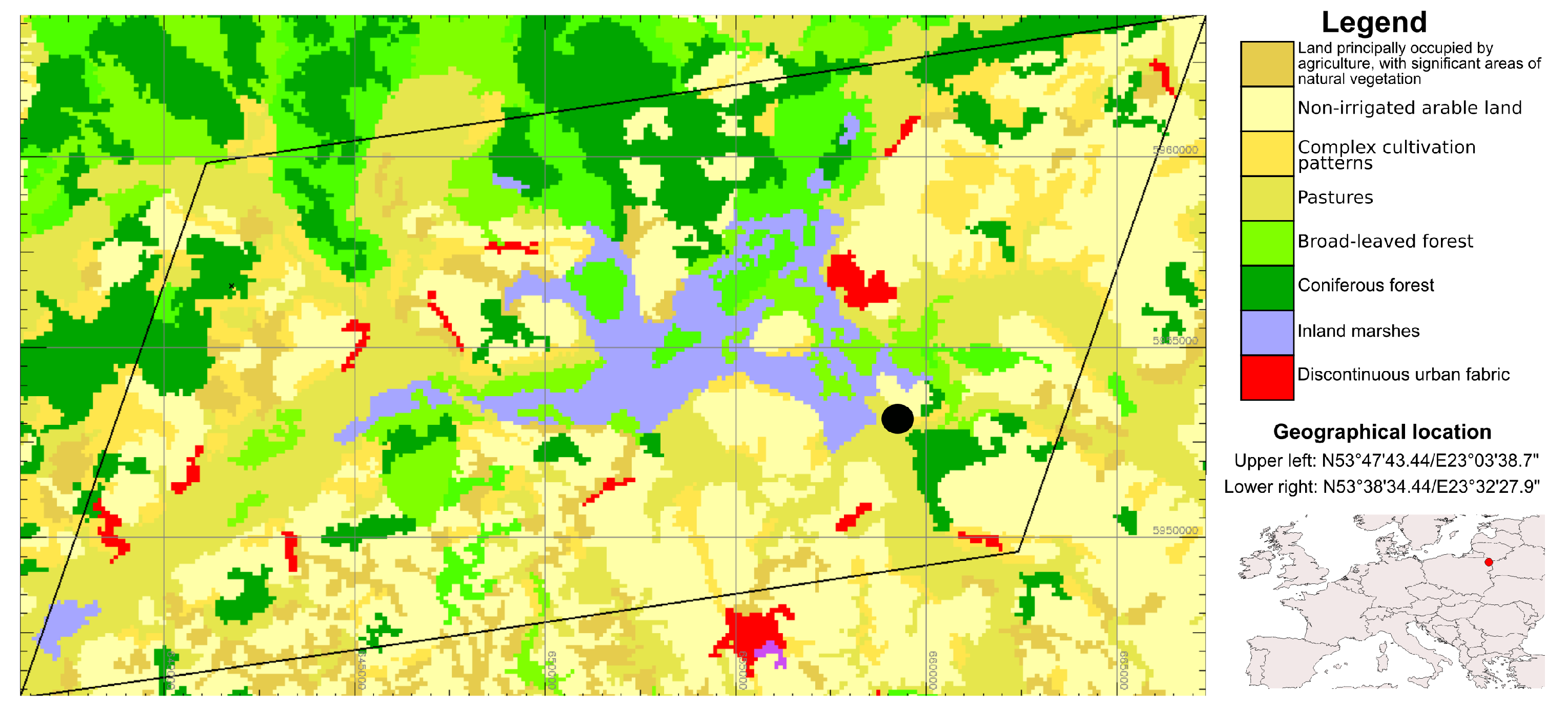
The study area in the Biebrza basin comprised over 35,000 hectares, indicated in the map of Figure 3. The map also shows the land cover classes in the study area according to the CORINE land cover map [24]. The simulations in this area were contrasted against in situ measurement conducted at a flux tower located in Rogozynek (53${}^{\circ }$42’8.19”, 23${}^{\circ }$24’46.9”).

2.3. Data Sources

2.3.1. Meteorological Variables

The meteorological forcing for the simulations on the sites listed in Table 1 was obtained from in situ measurements contained in the FLUXNET2015 dataset (https://fluxnet.fluxdata.org/data/fluxnet2015-dataset/) and ERA5, a dataset of reanalysed meteorological and atmospheric observation generated at the European Centre for Medium-Range Weather Forecasts (ECMWF) [25] (ERA stands for ECMWF Re-Analysis). Half-hourly data on incoming solar radiation ($S\downarrow$, $L\downarrow$) and wind speed were taken from FLUXNET2015. Other meteorological variables were taken from the hourly records of ERA5 as the in situ air temperature and relative humidity data series had gaps. The ERA5 meteorological data were then interpolated to match the half-hourly solar radiation time series. Data on soil moisture and soil temperature also were taken from ERA5 for 4 soil layers.

ERA5 was the main source of meteorological forcing for the simulation over the upper Biebrza basin as well. However, the radiation terms for the simulations over the Biebrza basin were taken from the LSA-SAF downwelling short and long solar radiation products [26,27]. These products are based on observations by the SEVIRI sensor onboard the geostationary Meteosat Second Generation Satellite (MSG) in the electromagnetic regions 0.3–4.0 μm and 4–100 μm, respectively. These products are generated with a 0.5 h temporal resolution.

2.3.2. Polar-Orbit Satellites

The amount of vegetation foliage in the canopy exerts a great impact on the composition of the ET flux. It determines, amongst other, the transpiration flux resulting from photosynthesis, the amount of rainfall water intercepted by the canopy, the soil water uptake, the resistance to wind currents, the fraction of $R_{net}$ stored in the upper soil layers, etc.

In order to account for vegetation dynamics and albedo, the ET model ingested estimates derived from observations by polar-orbit satellites. These products are able to capture the seasonal patterns of vegetation and are normally available at moderate/high spatial resolution. The model variables taken from polar-orbit satellites were leaf area index (LAI), albedo ($\alpha$) and fraction of vegetation cover. The LAI values were extracted from the dedicated product generated in the framework of the Copernicus Global Land Programme (CGLP) (https://land.copernicus.eu/) [28]. This product consists of a continuous archive of LAI estimates built on the basis of coupling the operation period of SPOT-V and PROBA-V [29]; which makes more than 20 years of global vegetation-related information. Albedo [30] and fraction of vegetation cover are part of the CGLP portfolio as well. The former was required in the computation of $R_{net}$, and the latter served as a basis for weighing the contribution of each tile within the cells.

The products used for the simulation over the sites in Table 1 had a spatial resolution of ∼1 km. The simulations over the upper part of the Biebrza basin were conducted over the grid of the PROBA-V imagery at an ∼300 m spatial resolution [31]. All needed RS products but albedo were available in the CGLP portfolio at an ∼300 m spatial resolution for the period starting in late 2013 (the start of operations of PROBA-V). The albedo values used at the ∼300 m resolution were obtained from the resampling of the albedo MODIS MCD43A2 product [32], which combines observations by the MODIS sensor onboard the TERRA and AQUA satellites.

2.3.3. Land Cover

A number of important model parameters (minimum stomatal resistance, root density in different soil layers and vegetation height, amongst others) was associated with the land cover. In this study, the Ecoclimap I database [33] was used to extract information on the type of ecosystem at each studied location in Table 1. The Ecoclimap database covers the globe at an ∼1 km spatial resolution. Every point on Earth is associated with an ecosystem type, which in turn is composed of tiles representing functional vegetation types, water bodies, bare soil, urban environments, impermeable surfaces or snow. The Ecoclimap I database also contains data on the occupation fraction of the different tiles in each ecosystem. This spatial information was taken from Ecoclimap I, and the actual parameter values associated with the tiles were the same as those used in the operational ET LSA-SAF product [34].

The information on land cover over the studied site in the upper Biebrza basin was obtained from a more recent version of the Ecoclimap database, the Ecoclimap Second-Generation (ECOCSG) [35]. Novel elements of ECOCSG with respect to older versions of Ecoclimap are: (a) higher spatial detail (∼300 m); and (b) each cell in the ECOCSG map corresponds to only one tile. The dataset was built on the basis of the ESA-CCI map and contains 33 land cover classes, out of which 9 are urban.

The criterion of the Ecoclimap database was followed for deriving the value of emissivity $\epsilon$ as a function of the fraction of vegetation cover ($fcov$): $\epsilon =fcov\ast 0.97+(1-fcov)\ast 0.94$.

Table 2. Overview of data sources to force the ET model at flux tower locations and across the study area in the upper Biebrza basin, Poland. The SPOT-Végétation (S-Vgt) and PROBA-V products were generated in the framework of the Copernicus Global Land Service at a 1 km and a 300 spatial resolution, respectively. LSA-SAF, Land Surface Analysis programme (LSA-SAF); ECOCSG, Ecoclimap Second-Generation.

Forcing Variable	Point Locations (FLUXNET2015 Sites)	Upper Biebrza Basin
Solar radiation	in situ measurement	LSA-SAF downwelling solar radiation
Air temperature and dew point temperature	ERA5	ERA5
Wind speed	in situ measurement	ERA5
Leaf Area Index	S-Vgt	PROBA-V
Albedo	S-Vgt	MODIS MCD43A2
Land cover	EcoclimapI	ECOCSG
Fraction of vegetation cover	S-Vgt	PROBA-V
Soil moisture	ERA5	ERA5
Soil temperature	ERA5	ERA5
Atmospheric pressure	ERA5	ERA5

presents an overview of the data sources described in the previous paragraphs and indicates the simulation domain (flux tower locations or upper Biebrza basin) where each data source was used.

2.4. Validation

The estimated daily ET was validated with in situ measurements at the sites listed in Table 1 and compiled in the FLUXNET2015 dataset. The $LE$ data actually used for the validation were selected based on the quality flag provided in FLUXNET2015 and were taken from series where no correction of energy balance closure was performed.

The validation data for the simulation over the upper Biebrza basin were obtained from measurements at a flux tower located within the study area, in the village of Rogozynek. This dataset proved useful in previous research studies concerning evaluation of surface energy balance and soil-vegetation-atmosphere transfer models [36] and finding a correlation between spectral indices and greenhouse gas fluxes [37].

The simulated data series were compared with the measurement at the flux towers on the basis of commonly used statistical parameters: root mean squared error, bias, coefficient of determination and the Nash–Sutcliffe efficiency coefficient (NSE) [38].

3. Results

3.1. Simulations at Flux Towers’ Locations

Table 3. Bias (mm/day), root mean squared error (RMSE) (mm/day), coefficient of determination ($r^2$) and the Nash–Sutcliffe efficiency index obtained from contrasting the simulated daily ET against in situ measurements at flux tower stations as compiled in the FLUXNET 2015 datasets.

Site Acronym	n	Bias	RMSE	${\mathit{r}}^2$	NSE
CRO
BE-Lon	2900	0.4364	0.7255	0.8788	0.5990
DE-Kli	2868	0.4216	0.7050	0.8965	0.3815
DE-RuS	598	−0.6404	0.9245	0.8608	0.4949
DE-Seh	1062	−0.3591	0.8058	0.8178	0.5724
US-ARM	3222	−0.4432	0.8462	0.7456	0.3740
DBF
FR-Fon	3135	−0.5444	0.9771	0.8162	0.5118
JP-MBF	654	−0.0236	0.8592	0.7733	0.5629
PA-SPn	752	−0.8814	1.1599	0.6726	−0.4074
EBF
CN-Din	889	0.3165	0.7904	0.7847	0.2972
FR-Pue	4384	−0.0521	0.4992	0.7960	0.6217
GF-Guy	3361	−0.3473	0.7987	0.7341	0.2736
GH-Ank	542	0.4852	1.1482	0.4232	−0.1056
MY-PSO	2153	−0.0041	0.5075	0.8176	0.5281
ENF
AR-Vir	496	−0.7192	1.1601	0.7831	0.3429
CA-SF2	1296	−0.2089	0.6315	0.9102	0.7878
DE-Obe	2005	0.2402	0.6223	0.8847	0.6301
DE-Tha	5265	0.3345	0.8196	0.8615	0.1901
FI-Hyy	4913	0.3351	0.6696	0.9066	0.4794
FI-Let	1023	0.0142	0.4510	0.9176	0.8301
NL-Loo	4890	−0.2528	0.7278	0.7641	0.4363
RU-Fyo	4714	0.1603	0.6354	0.8682	0.6950
US-Me6	1075	−0.4521	0.8095	0.5984	0.0661
GRA
AU-DaP	1528	−0.2262	0.622	0.9457	0.8767
AU-Stp	1484	−0.2482	0.8504	0.7831	0.5754
US-SRG	1931	0.1598	0.5926	0.8315	0.6551
MF
BE-Bra	4372	0.4162	0.6780	0.8884	0.3196
BE-Vie	4011	0.4915	0.7743	0.9334	0.3193
CA-Gro	3401	0.2931	0.6556	0.8988	0.6112
CH-Lae	3088	−0.1878	1.061	0.8084	0.6013
JP-SMF	1338	−0.6976	0.9769	0.8026	0.2297
US-SRC	1599	−0.1738	0.5094	0.7407	0.4352
OSH
CA-NS6	1329	0.2942	0.5131	0.9233	0.4720
CA-SF3	1606	−0.1217	0.4992	0.8977	0.7790
US-Sta	873	−0.5572	1.1356	0.5526	0.0715
SAV
AU-ASM	852	−0.4086	0.7206	0.7636	0.3541
AU-DaS	1814	0.3992	0.6449	0.8707	0.6070
AU-Dry	1104	−0.2066	0.7394	0.7897	0.5387
CG-Tch	892	0.3198	0.5680	0.8634	0.6229
SD-Dem	686	−0.6737	1.2285	0.6484	0.1598
WET
DE-Spw	1119	0.1993	0.4882	0.9307	0.8347
RU-Che	529	−0.2045	0.6828	0.4837	0.1463
WSA
AU-Ade	529	−1.2595	1.4166	0.9093	0.1721
AU-How	3392	−0.3221	0.7145	0.8622	0.6778
US-SRM	3374	−0.501	0.7656	0.7559	0.2360

presents statistical parameters that indicate the ability of the ET model to simulate the daily ET derived from the measurement at flux towers.

In most of the studied sites, the simulated daily ET exhibited high correlation with the validation data. This translated into $r^2$ values greater than 0.75 in most of the sites in all plant functional types. The $r^2$ values were even higher than 0.9 in various sites. In the best cases, high correlation between simulation and validation data series was accompanied by high NSE values, which indicated similarity between modelled and measured values; i.e., low bias and low RMSE. Such a condition was present in sites associated with all considered plant functional types.

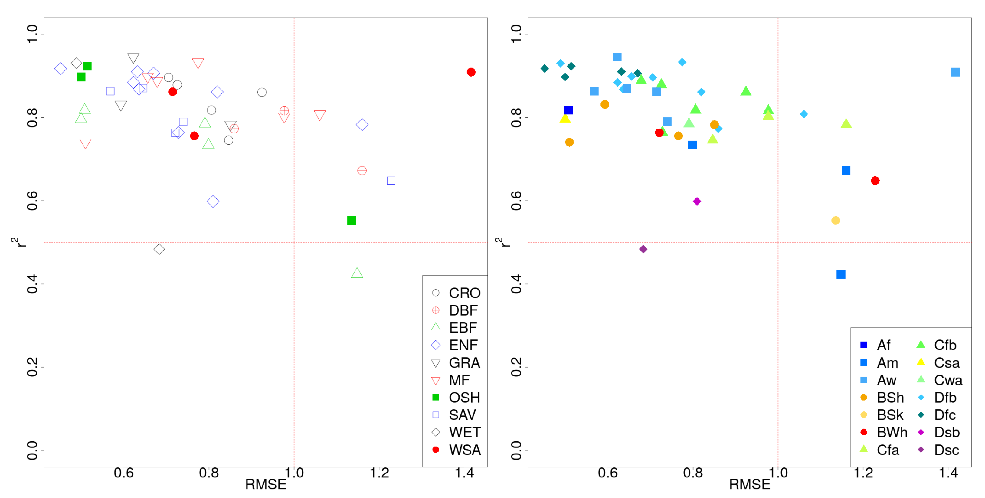
The plots of Figure 4 depict the results of the simulations in terms of the obtained $r^2$ and RMSE per site in association with the corresponding plant functional type and climatic zone. These plots show that all plant functional types were represented in the $r^2$ > 0.5 and RMSE < 1 graph quadrant. Most of the simulations falling outside that area exhibited RMSE values higher than one and belonged to climatic zones associated with tropical regions or dry climate.

The plots in Figure 5 depict the variability in simulated and validation daily ET throughout the year for sites in the considered plant functional types. Although this analysis could vary from site to site, the examples shown in Figure 5 indicate the nature of the similarities and dissimilarities between simulations and validation data expressed in the statistical parameters of Table 3. In general, the plots show the ability of the model to capture the most important vegetation phenology events; namely, the rise and decline of the growing season. Likewise, the plots show the periods of over- or under-estimation of the actual ET. For instance, the simulations for Brasschaat Belgium (BE-Bra) tended to be higher than the measured values; the model tended to slightly overestimate ET in Tchizalamou Congo (CG-Tch) during the period of lowest ET rates; a short period where the highest ET rates in Puechabon France (FR-Pue) were underestimated, etc. Nevertheless, the plots show an important degree of overlap between the areas representing the variability of the simulated and validation datasets. The output of daily ET simulations over the sites in Table 1 are made available to the reader as supplementary material of this article.

3.2. Simulations in the Upper Biebrza Basin

The simulations conducted for the years 2015–2016 at the location of the flux tower in Rogozynek, in the upper part of the Biebrza basin, exhibited a positive bias of 0.1685 mm/day with a root mean squared error equal to 0.6930 mm/day (n = 311). The coefficient of determination ($r^2$) was equal to 0.8705, and the value of the Nash–Sutcliffe Efficiency index was 0.6598. The time series of simulated and validation daily ET are presented in Figure 6.

The statistical parameters presented in the previous paragraph and the features of the time series shown in Figure 6 indicated overall good agreement between the output of the simulations and the in situ measured data. The simulated time series correlated well with the validation data, and the time series plot allowed the identification of the particular periods of the growing season where both time series differed the most.

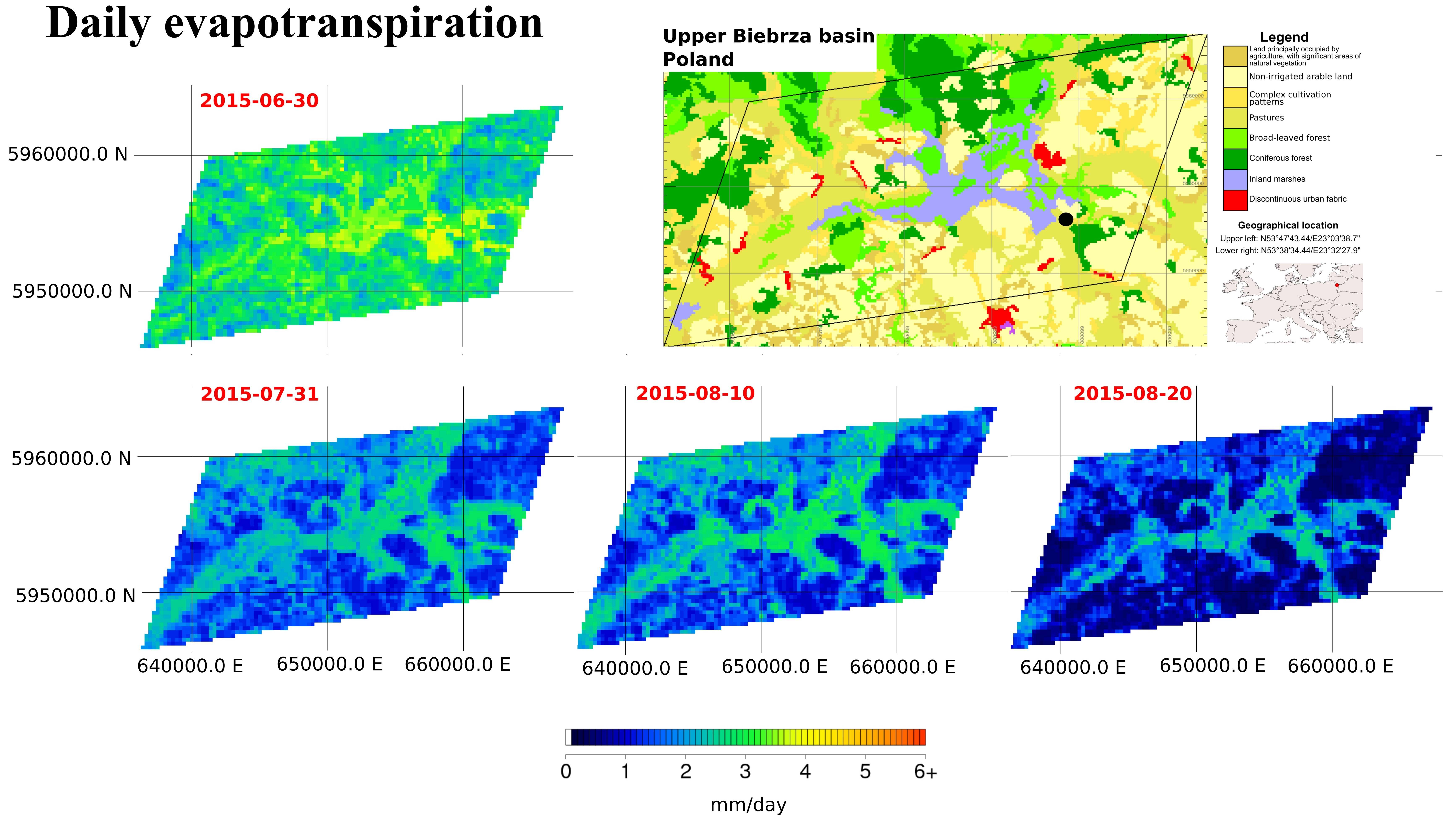
The modelled daily ET at the location of the flux tower in Rogozynek was extracted from simulations conducted across a larger area at a 300 m spatial resolution; specifically, over the grid of PROBA-V 300 m imagery. Examples of those simulations for the growing season 2015 are presented in Figure 7.

Although no means were available to validate simulations outside the footprint of the flux tower, the daily ET maps of Figure 7 depict spatial patterns that could be expected in the considered dates and for the landscape arrangement of the study area (see Figure 3). The highest ET rates were located in the river channel and adjacent wetlands. The maps also allow distinguishing the ET patterns in the forest area in the northwest side of the study area, as well as a more scattered pattern in other areas where mosaics of grassland and crops were located.

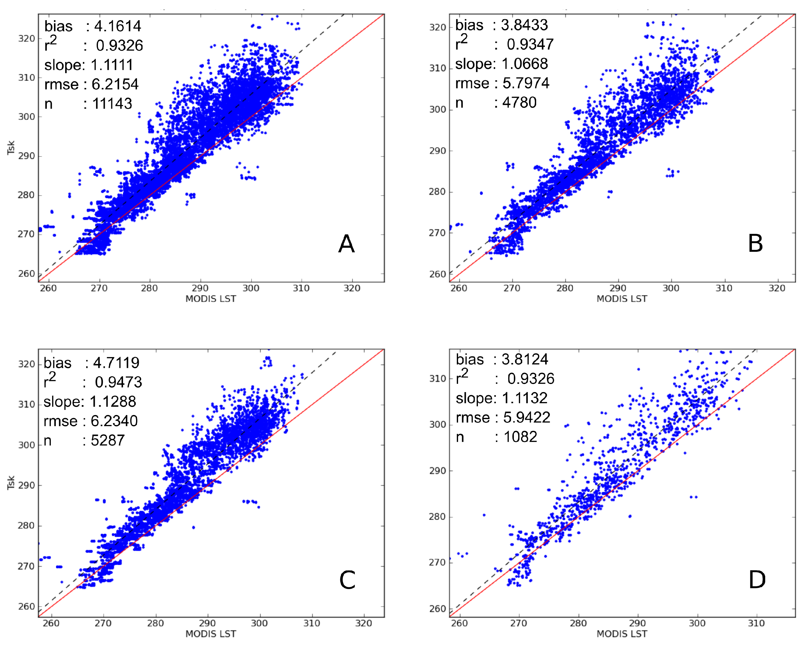
As described in Section 2.1, the ET algorithm in this study did not ingest LST as part of the forcing dataset. It rather estimated the $T_{sk}$ term of the energy balance through an iterative process. One should expect, however, that the estimate of $T_{sk}$ would be similar in magnitude and shape to LST obtained from spaceborne observations. This could serve as an additional test for the coherence of the simulations. Figure 8 presents scatterplots that contrast, for four land cover classes, the $T_{sk}$ estimated internally by the model against LST data retrieved from the MODIS MOD11A1 LST daily product at a 1 km resolution [39].

The comparison of $T_{sk}$ with MODIS LST does not imply that the latter should be considered as reference for validation. Nevertheless, finding high correlation between these two independent and different in nature datasets is a positive indicator of coherence in the results.

4. Discussion

The main motivation for implementing the LSA-SAF ET model at a higher spatial resolution setting (∼300 m and ∼1 km) was rooted in the need for continuous estimates of land surfaces variables at useful spatial resolutions for monitoring management units (forest stands, agriculture regions, wetlands, protected areas, etc.). The results presented in the previous section revealed the potential of the approach followed here and confirmed the value of a number of principles in the LSA-SAF ET model that proved useful and valid in the generation of daily ET estimates at a sub-kilometre spatial resolution. At least two aspects can be underlined in that respect:

(a) The fruitful combination of geostationary and polar-orbit satellites towards the generation of ET estimates: The approach followed in this study strived to utilise spaceborne information optimally such that ET drivers exhibiting high variability during the day (namely, short and long wave incoming radiation) would be obtained from RS data sources based on geostationary satellites. Other ET determinants that were closely related to land cover and exhibited seasonal temporal patterns (like LAI, albedo, fraction of vegetation cover) may be better derived from high spatial resolution data sources, i.e., polar-orbit satellites like SPOT-V, PROBA-V and, more recently, Sentinel-2 and Sentinel-3.

(b) The continuity element in daily ET estimates was emphasized in the Introduction Section of this article. The non-dependency of the LSA-SAF ET algorithm on RS-based LST was a crucial factor in reducing the gaps in the generated time series due to the high sensitivity of spaceborne LST to cloudiness. The comparison with MODIS LST (Figure 8) indicated that this approach yielded good results.

Moving towards more spatial detail entails the challenge of building forcing datasets compatible with the target spatial resolution. The advent of spatial missions with enhanced performance has contributed to make this possible. Nevertheless, currently available data of soil moisture and/or soil characteristics might still be too coarse, with respect to the target spatial resolution, and may result in poor simulations of ET. This might partially explain the somewhat low statistical scores in some sites in climatic zones where soil moisture was the main driver of ET. The discrepancy might only be present in particular periods of the year, as shown in Figure 9, where the simulated daily ET rates were underestimated during the dry season in that part of the world. This was, in turn, related to underestimating the actual available volume of soil water for transpiration. It also illustrates the sensitivity of the model to proper information on soil moisture and soil physical properties determining the actual availability of soil water.

This study considered the ERA5 dataset as the source of soil moisture. Future implementations should test the performance of other soil moisture data sources. In this respect, the approach adopted in the most recent version of the LSA-SAF ET product is worth considering. This development was based on the principle of thermal inertia to derive estimates of soil moisture and relied on LST data derived from the geostationary MSG satellite [40]. This approach proved successful in arid and semi-arid areas.

The daily ET simulations over the upper Biebrza basin were a first experience in the use of ECOCSG as forcing of the ET model presented here. The simulations of this study adopted the parameterization of the LSA-SAF ET model and applied it at a higher spatial resolution. Future simulations based on ECOCSG, and implemented in other regions, might benefit from revising and fine tuning the parameters as this dataset included new vegetation types that were not present in previous versions of Ecoclimap.

A Glance into the Future

The results of this study, as well as the findings in previous research [13], showed the suitability of products derived from SPOT-V and PROBA-V observations to integrate the forcing dataset of the ET model implemented here. The PROBA-V operational phase allowed taking a step towards more spatial detail in daily ET simulations. However, in view of the upcoming end of the operational life of PROBA-V, it is pertinent to state future implementations of this algorithm in terms of products derived from Sentinel-3 observations.

The ET algorithm used in this study ingested RS products derived from observations of optical sensors. Therefore, the Sentinel-3 sensor of interest is the Ocean and Land Color Instrument (OLCI), which senses the Earth in 21 spectral bands in the region 400–1020 nm. This region overlaps with three of the four bands of PROBA-V. The full resolution products are delivered at a 300 m spatial resolution.

Including OLCI observations in ET simulations, as those performed in this study, would require the translation of its spectral information into broad-band albedo, LAI and fraction of vegetation cover. These parameters are the basic ingredients of the LSA-SAF ET algorithm, as well as of other similar tools simulating different processes of the land surface. Although currently delivered OLCI data contain the necessary spectral information for deriving such parameters, the interest of the land surface modelling community in OLCI could be stimulated, making it part of the list of standard delivered OLCI products. Previous efforts in the derivation of land biophysical values with MERIS could be the starting point [41,42].

Currently, the OLCI Global and Terrestrial Chlorophyll Indices (OGVI and OTCI, respectively) are available as L2 products. These products are intended to give continuity to the analogous MGVI and MTCI based on ENVISAT/MERIS [43,44]. The ET LSA-SAF algorithm is not designed to ingest any of these products; moreover, none of them is a full equivalent of LAI. However, MGVI—the precursor of OGVI—represented FAPAR [45], which is known to be related to LAI [46]. The maps and plots in Figure 10 show the existence of common spatial patterns and a substantial degree of correlation between OGVI and PROBA-V LAI in our study area in Biebrza, Poland. On the basis of the relationship PROBA-V LAI and OLCI OGVI, one could derive empirical models to estimate LAI and implement the LSA-SAF ET for local or regional studies. Estimates of the fraction of vegetation cover and albedo could be approached in a similar way for fast and local appraisals. As suggested above, the full exploitation of OLCI observations in land surface models would be eased by developing such biophysical parameters in an operational framework.

5. Conclusions

This study aimed at conducting daily ET simulations at an ∼1 km spatial resolution in a variety of climate and land cover conditions. The approach relied on the principles behind the LSA-SAF ET algorithm and the adequacy of biophysical variables derived from SPOT-V and PROBA-V to integrate the forcing dataset.

The approach delivered satisfactory results when contrasted against measurements done at eddy covariance stations. The obtained daily ET estimates correlated well with the validation time series, and the comparison of the internally computed $T_{sk}$ in the upper Biebrza basin with spaceborne LST exhibited great similarity. These were all indicators that featured the approach presented here as a promising tool to support applications where continuous daily ET at sub-kilometre spatial resolution may be required (e.g., watershed management, water accounting, regional drought monitoring, etc.).

The results also pointed to avenues of future research envisaging further improvement of the model and the exploitation of OLCI Sentinel-3 observations. The adoption of ECOCSG in the simulations in the upper Biebrza basin delivered good results; future tests in other climate zones and landscape configurations should be performed to verify its suitability in other conditions. In parallel, the best methods to translate current OLCI products into biophysical parameters to feed the ET algorithm (and other land surface models) should be investigated. Moreover, the step towards higher resolution might entail the upgrade of some land cover-related parameters, which may help with reducing the error of the simulations.

References

- Zhang, C.; Liu, J.; Dong, T.; Pattey, E.; Shang, J.; Tang, M.; Cai, H.; Saddique, Q. Coupling Hyperspectral Remote Sensing Data with a Crop Model to Study Winter Wheat Water Demand. Remote Sens. 2019, 11, 1648. [Google Scholar] [CrossRef]
- Tirivarombo, S.; Osupile, D.; Eliasson, P. Drought monitoring and analysis: Standardised Precipitation Evapotranspiration Index (SPEI) and Standardised Precipitation Index (SPI). Phys. Chem. Earth Parts A/B/C 2018, 106, 1–10. [Google Scholar] [CrossRef]
- Wu, X.; Wang, P.; Huo, Z.; Wu, D.; Yang, J. Crop Drought Identification Index for winter wheat based on evapotranspiration in the Huang-Huai-Hai Plain, China. Agric. Ecosyst. Environ. 2018, 263, 18–30. [Google Scholar] [CrossRef]
- Kyatengerwa, C.; Kim, D.; Choi, M. A national-scale drought assessment in Uganda based on evapotranspiration deficits from the Bouchet hypothesis. J. Hydrol. 2020, 580, 124348. [Google Scholar] [CrossRef]
- Wu, B.; Jiang, L.; Yan, N.; Perry, C.; Zeng, H. Basin-wide evapotranspiration management: Concept and practical application in Hai Basin, China. Agric. Water Manag. 2014, 145, 145–153. [Google Scholar] [CrossRef]
- Petropoulos, G.; Ireland, G.; Lamine, S.; Griffiths, H.; Ghilain, N.; Anagnostopoulos, V.; North, M.; Srivastava, P.; Georgopoulou, H. Operational evapotranspiration estimates from SEVIRI in support of sustainable water management. Int. J. Appl. Earth Obs. Geoinf. 2016, 49, 175–187. [Google Scholar] [CrossRef]
- Qiu, G.; LI, H.; Zhang, Q.; Chen, W.; Liang, X.; Li, X. Effects of Evapotranspiration on Mitigation of Urban Temperature by Vegetation and Urban Agriculture. J. Integr. Agric. 2013, 12, 1307–1315. [Google Scholar] [CrossRef]
- Qiu, G.; Tan, S.; Wang, Y.; Yu, X.; Yan, C. Characteristics of Evapotranspiration of Urban Lawns in a Sub-Tropical Megacity and Its Measurement by the ‘Three Temperature Model + Infrared Remote Sensing’ Method. Remote Sens. 2017, 9, 502. [Google Scholar]
- Fisher, J.; Melton, F.; Middleton, E.; Hain, C.; Anderson, M.; Allen, R.; McCabe, M.; Hook, S.; Baldocchi, D.; Townsend, P.; et al. The future of evapotranspiration: Global requirements for ecosystem functioning, carbon and climate feedbacks, agricultural management, and water resources. Water Resour. Res. 2017, 53, 2618–2626. [Google Scholar] [CrossRef]
- Liou, Y.; Kar, S. Evapotranspiration estimation with remote sensing and various surface energy balance algorithms—A review. Energies 2014, 7, 2821–2849. [Google Scholar] [CrossRef]
- Bórnez, K.; Descals, A.; Verger, A.; Peñuelas, J. Land surface phenology from VEGETATION and PROBA-V data. Assessment over deciduous forests. Int. J. Appl. Earth Obs. Geoinf. 2020, 84, 10174. [Google Scholar] [CrossRef]
- Meroni, M.; Fasbender, D.; Balaghi, R.; Dali, M.; Haffani, M.; Haythem, I.; Hooker, J.; Lahlou, M.; Lopez-Lozano, R.; Mahyou, H.; et al. Evaluating NDVI data continuity between SPOT-VEGETATION and PROBA-V missions for operational yield forecasting in North African Countries. IEEE Trans. Geosci. Remote Sens. 2016, 54, 795. [Google Scholar] [CrossRef]
- Barrios, J.; Ghilain, N.; Arboleda, A.; Sachs, T.; Gellens-Meulenberghs, F. Daily evapotranspiration at sub-kilometre spatial resolution by combining observations from geostationary and polar-orbit satellites. Int. J. Remote Sens. 2018, 39, 8984–9003. [Google Scholar] [CrossRef]
- Trigo, I.; Dacamara, C.; Viterbo, P.; Roujean, J.L.; Olesen, F.; Barroso, C.; Camacho-de Coca, F.; Carrer, D.; Freitas, S.; García-Haro, J.; et al. The Satellite Application Facility for Land Surface Analysis. Int. J. Remote Sens. 2011, 32, 2725–2744. [Google Scholar] [CrossRef]
- Ghilain, N.; Arboleda, A.; Gellens-Meulenberghs, F. Evapotranspiration modelling at large scale using near-real time MSG SEVIRI derived data. Hydrol. Earth Syst. Sci. 2011, 15, 771–786. [Google Scholar] [CrossRef]
- Ghilain, N.; Arboleda, A.; Sepulcre-Cantò, G.; Batelaan, O.; Ardö, J.; Gellens-Meulenberghs, F. Improving evapotranspiration in a land surface model using biophysical variable derived from MSG/SEVIRI satellite. Hydrol. Earth Syst. Sci. 2012, 16, 2567–2583. [Google Scholar] [CrossRef]
- Sepulcre-Cantó, G.; Vogt, J.; Arboleda, A.; Antofie, T. Assessment of the EUMETSAT LSA-SAF evapotranspiration product for drought monitoring in Europe. Int. J. Appl. Earth Obs. Geoinf. 2014, 30, 190–202. [Google Scholar] [CrossRef]
- Hu, G.; Jua, L.; Menenti, M. Comparison of MOD16 and LSA-SAF MSG evapotranspiration products over Europe for 2011. Remote Sens. Environ. 2014, 156, 510–526. [Google Scholar] [CrossRef]
- Minacapilli, M.; Consoli, S.; Vanella, D.; Ciraolo, G.; Motisi, A. A time domain triangle method approach to estimate actual evapotranspiration: Application in a Mediterranean region using MODIS and MSG-SEVIRI products. Remote Sens. Environ. 2016, 174, 10–23. [Google Scholar] [CrossRef]
- Sun, Z.; Gebremichael, M.; Ardö, J.; Nickless, A.; Caquet, B.; Merboldh, L.; Kutschi, W. Estimation of daily evapotranspiration over Africa using MODIS/Terra and SEVIRI/MSG data. Atmos. Res. 2012, 112, 35–44. [Google Scholar] [CrossRef]
- Martins, J.; Trigo, I.; Ghilain, N.; Jimenez, C.; Göttsche, F.; Ermida, S.; Olesen, F.; Gellens-Meulenberghs, F.; Arboleda, A. An All-Weather Land Surface Temperature Product Based on MSG/SEVIRI Observations. Remote Sens. 2019, 11, 3044. [Google Scholar] [CrossRef]
- Oak Ridge National Laboratory Distributed Active Archive Center (ORNL DAAC). FLUXNET Portal. 2014. Available online: http://fluxnet.ornl.gov/ (accessed on 15 January 2014).
- Beck, H.; Zimmermann, N.; McVicar, T.; Vergopolan, N.; Berg, A.; Wood, E. Present and future Köppen–Geiger climate classification maps at 1-km resolution. Sci. Data 2018, 5, 180214. [Google Scholar] [CrossRef] [PubMed]
- European Environment Agency. CORINE Land Cover 2000. Available online: http://www.eea.europa.eu/themes/landuse/clc-download (accessed on 15 January 2014).
- Copernicus Climate Change Service. ERA5: Fifth Generation of ECMWF Atmospheric Reanalysis of the Global Climate. Copernicus Climate Change Service Climate Data Store (CDS). 2017. Available online: https://cds.climate.copernicus.eu/cdsapp#!/dataset/reanalysis-era5-land?tab=overview (accessed on 15 October 2019).
- Méteo-France/CNRM. Algorithm Theoretical Basis Document—Downwelling Surface Shortwave Flux (DSSF) Product. LSA-SAF. 2012. Available online: http://landsaf.ipma.pt (accessed on 15 November 2019).
- Trigo, I.; Freitas, S.; Barroso, C.; Monteiro, I.; Viterbo, P. Algorithm Theoretical Basis Document—Downwelling Longwave Flux (DSSF) Product. LSA-SAF. 2009. Available online: http://landsaf.ipma.pt (accessed on 15 November 2019).
- Jutz, S.; Milagro-Pérez, M. 1.06—Copernicus Program. In Comprehensive Remote Sensing; Liang, S., Ed.; Elsevier: Oxford, UK, 2018; pp. 150–191. [Google Scholar]
- Gio-Global Land Component Lot1 Consortium. Algorithm Theorethical Basis Document—Leaf Area Index (LAI), Fraction of Absorbed Photosynthetically Active Radiation (FAPAR), Fraction of Vegetation Cover (FCover) Collection 1 km Version 2. Copernicus Programme. 2019. Available online: http://land.copernicus.eu/global/sites/cgls.vito.be/files/products/CGLOPS1_ATBD_LAI1km-V2_I1.41.pdf (accessed on 20 August 2019).
- Roujean, J.; Leon-Tavares, J.; Smets, B.; Claes, P.; Camacho De Coca, F.; Sanchez-Zapero, J. Surface albedo and tocr 300m products from PROBA-V instrument in the framework of Copernicus Global Land Service. Remote Sens. Environ. 2018, 215, 57–73. [Google Scholar] [CrossRef]
- ImagineS Consortium. ATBD for LAI, FAPAR, and FCOVER from PROBA-V Products at 300m Resolution (GEOV3). Copernicus Programme. 2016. Available online: http://land.copernicus.eu/global/sites/cgls.vito.be/files/products/ImagineS_RP2.1_ATBD-LAI300m_I1.73.pdf (accessed on 20 August 2019).
- Schaaf, C.; Wang, Z. MCD43A2 MODIS/Terra+Aqua BRDF/Albedo Daily L3 Global—500m V006[Data Set], 2015. NASA EOSDIS Land Processes DAAC. Available online: https://doi:10.5067/MODIS/MCD43A2.006 (accessed on 16 April 2018).
- Masson, V.; Champeaux, J.L.; Chauvin, F.; Meriguet, C.; Lacaze, R. A global database of land surface parameters at 1-km resolution in meteorological and climate models. J. Clim. 2003, 16, 1261–1282. [Google Scholar] [CrossRef]
- Royal Meteorological Institute of Belgium. Algorithm Theoretical Basis Document—Evapotranspiration (MET) Product—Daily MET (DMET) Product. LSA-SAF. 2010. Available online: http://landsaf.meteo.pt (accessed on 15 January 2019).
- Méteo-France/CNRS. ECOCLIMAP-SG. 2018. Available online: https://opensource.umr-cnrm.fr/projects/ecoclimap-sg/wiki (accessed on 15 November 2019).
- Mallick, K.; Wandera, L.; Bhattarai, N.; Hostache, R.; Kleniewska, M.; Chormanski, J. A Critical Evaluation on the Role of Aerodynamic and Canopy–Surface Conductance Parameterization in SEB and SVAT Models for Simulating Evapotranspiration: A Case Study in the Upper Biebrza National Park Wetland in Poland. Water 2018, 10, 1753. [Google Scholar] [CrossRef]
- Ciȩżkowski, W.; Berezowski, T.; Kleniewska, M.; Chormański, J. Carbon Dioxide and Water Vapour Fluxes of a Alkaline Fen and Their Dependence on Reflectance. In Proceedings of the IGARSS 2018—2018 IEEE International Geoscience and Remote Sensing Symposium, Valencia, Spain, 22–27 July 2018; pp. 9253–9256. [Google Scholar] [CrossRef]
- Nash, J.; Sutcliffe, J. River flow forecasting through conceptual models part I -A discussion of principles. J. Hydrol. 1970, 10, 282–290. [Google Scholar] [CrossRef]
- Wan, Z.; Hook, S.; Hulley, G. MOD11A1 MODIS/Terra Land Surface Temperature/Emissivity Daily L3 Global 1km SIN Grid V006 [Data Set], 2015. NASA EOSDIS Land Processes DAAC. Available online: https://doi.org/10.5067/MODIS/MOD11A1.006 (accessed on 16 April 2018).
- Ghilain, N.; Arboleda, A.; Batelaan, O.; Ardö, J.; Trigo, I.; Barrios, J.; Gellens-Meulenberghs, F. A New Retrieval Algorithm for Soil Moisture Index from Thermal Infrared Sensor On-Board Geostationary Satellites over Europe and Africa and Its Validation. Remote Sens. 2019, 11, 1968. [Google Scholar] [CrossRef]
- Tum, M.; Günther, K.; Böttcher, M.; Baret, F.; Bittner, M.; Brockmann, C.; Weiss, M. Global Gap-Free MERIS LAI Time Series (2002–2012). Remote Sens. 2016, 8, 69. [Google Scholar] [CrossRef]
- Bacour, C.; Baret, F.; Béal, D.; Weiss, M.; Pavageau, K. Neural network estimation of LAI, fAPAR, fCover and LAIxCab, from top of canopy MERIS reflectance data: Principles and validation. Remote Sens. Environ. 2006, 105, 313–325. [Google Scholar] [CrossRef]
- Dash, J.; Curran, P. Evaluation of the MERIS terrestrial chlorophyll index (MTCI). Adv. Space Res. 2007, 39, 100–104. [Google Scholar] [CrossRef]
- Gobron, N.; Pinty, B.; Verstraete, M.; Govaerts, Y. The MERIS Global Vegetation Index (MGVI): Description and preliminary application. Int. J. Remote Sens. 1999, 20, 1917–1927. [Google Scholar] [CrossRef]
- Gobron, N.; Bernard, P.; Mélin, F.; Taberner, M.; Verstraete, M.; Robustelli, M.; Widlowski, J. Evaluation of the MERIS/ENVISAT FAPAR product. Adv. Space Res. 2007, 39, 105–115. [Google Scholar] [CrossRef]
- Disney, M.; Muller, J.; Kharbouche, S.; Kaminski, T.; Voßbeck, M.; Lewis, P.; Pinty, B. A New Global fAPAR and LAI Dataset Derived from Optimal Albedo Estimates: Comparison with MODIS Products. Remote Sens. 2016, 8, 275. [Google Scholar] [CrossRef]
Figure 1.
General procedure for ET estimation where: : latent heat flux; : sensible heat flux; ground heat flux; : albedo; and : downwelling short and long wave solar radiation; : emissivity; : skin temperature; : soil moisture; : meteorological forcing; : parameters related to land cover.
Figure 2.
Location of flux towers considered in this study and the Köppen–Geiger climate classification [
23].
Figure 3.
Land cover (according to the CORINE land cover map) and location of the study area in the upper Biebrza basin, Poland. The black dot represents the location of the flux tower in Rogozynek.
Figure 4.
Scatterplot of and RMSE of simulated daily ET indicating the corresponding PFT (left) and the Köppen–Geiger climate class (right).
Figure 5.
Variability of daily ET as measured at the flux towers (light blue area) and simulated (shaded area). Variability was computed as the average ± the standard deviation.
Figure 6.
Daily ET as modelled at a 300 m spatial resolution and as obtained from in situ measurements at the flux tower in Rogozynek, Poland.
Figure 7.
Daily ET in the upper Biebrza basin at a 300 m spatial resolution for different dates in 2015.
Figure 8.
Scatterplots of MODIS LST and the skin temperature () internally estimated by the model. (A) Crops; (B) pastures; (C) wetlands; (D) complex cultivation patterns.
Figure 9.
Variability of daily ET as measured at the flux towers (light blue area) and simulated (shaded area) at Sardinilla plantation, Panama (PA-Spn).
Figure 10.
PROBA-V LAI (300 m resolution), OLCI Global VI (OGVI) and a scatterplot of both variables over the upper Biebrza basin, Poland, on 2 May 2016 and 11 July 2016.