Article

Spatial Attraction Models Coupled with Elman Neural Networks for Enhancing Sub-Pixel Urban Inundation Mapping

1
School of Remote Sensing and Information Engineering, Wuhan University, Wuhan 430079, China
2
Commonwealth Scientific and Industrial Research Organisation (CSIRO) Land and Water, Canberra 2601, Australia
3
Fenner School of Environment and Society, The Australian National University, Canberra 2601, Australia
4
College of Urban and Environmental Sciences, Northwest University, Xi’an 710127, China
5
Chongqing Engineering Research Center for Remote Sensing Big Data Application, School of Geographical Sciences, Southwest University, Chongqing 400715, China
*
Author to whom correspondence should be addressed.
Remote Sens. 2020, 12(13), 2068; https://doi.org/10.3390/rs12132068
Submission received: 27 April 2020 / Revised: 22 June 2020 / Accepted: 22 June 2020 / Published: 27 June 2020
(This article belongs to the Special Issue New Advances on Sub-pixel Processing: Unmixing and Mapping Methods)

Abstract

:
Urban flooding is one of the most costly and destructive natural hazards worldwide. Remote-sensing images with high temporal resolutions have been extensively applied to timely inundation monitoring, assessing and mapping, but are limited by their low spatial resolution. Sub-pixel mapping has drawn great attention among researchers worldwide and has demonstrated a promising potential of high-accuracy mapping of inundation. Aimed to boost sub-pixel urban inundation mapping (SUIM) from remote-sensing imagery, a new algorithm based on spatial attraction models and Elman neural networks (SAMENN) was developed and examined in this paper. The Elman neural networks (ENN)-based SUIM module was developed firstly. Then a normalized edge intensity index of mixed pixels was generated. Finally the algorithm of SAMENN-SUIM was constructed and implemented. Landsat 8 images of two cities of China, which experienced heavy floods, were used in the experiments. Compared to three traditional SUIM methods, SAMENN-SUIM attained higher mapping accuracy according not only to visual evaluations but also quantitative assessments. The effects of normalized edge intensity index threshold and neuron number of the hidden layer on accuracy of the SAMENN-SUIM algorithm were analyzed and discussed. The newly developed algorithm in this study made a positive contribution to advancing urban inundation mapping from remote-sensing images with medium-low spatial resolutions, and hence can favor urban flood monitoring and risk assessment.

Graphical Abstract

1. Introduction

Urban flooding is one of the most costly and destructive natural hazards worldwide, which poses a great threat to urban economic development and human safety [1,2]. Due to global warming and urbanization, the risks of urban inundation are expected to increase in the future [3]. Therefore, urban inundation mapping, which can obtain inundation distribution information for flood monitoring and risk assessment [4,5,6,7], has become increasingly important. High temporal resolution remote-sensing images have been extensively applied to timely inundation mapping and monitoring in recent years [8,9,10]. Nevertheless, the mapping accuracy of urban inundation is substantially compromised due to the low spatial resolutions of such images, which in a certain degree constrains the application of those valuable high temporal resolution remote-sensing data in flooding inundation mapping.
Sub-pixel urban inundation mapping (SUIM) can acquire the spatial distribution of urban inundation at a sub-pixel scale by detailing the spatial information structure inside a pixel to, therefore, boost the accuracy of inundation mapping. SUIM maximizes spatial dependence while maintaining the original proportion of urban inundation within the mixed pixel. Sub-pixel mapping is one hot point in the remote sensing and related fields. Numerous methods and improvements have been established and acquired, such as approaches based on genetic algorithm [11], spatial attraction models (SAM) [12,13], optimal endmember [14], spectral-spatial model [15], support vector machine (SVM) [16] and artificial neural networks [16,17,18]. Li et al. proposed an enhanced SUIM based on the fusion of SVM and general regression neural network [16]. Su integrated a scale-invariant feature of fractal geometry into the Hopfield neural network for sub-pixel mapping [17]. Arun et al. proposed convolutional network architectures for sub-pixel mapping of drone-derived images [18]. Nevertheless, SUIM in urban environments has been retained as a challenging research topic, because ground targets in urban remote-sensing images are complex.
SAM is simple and has explicit physical denotation, so it is a well-known approach in the sub-pixel mapping field [13]. Spatial attraction is defined to calculate the spatial correlation between a sub-pixel within a central pixel and the surrounding pixels of the central pixel. SAM is effectively an unsupervised algorithm, which does not require the prior knowledge of mixed pixels, such as their spatial structure, and does not need training samples. However, SAM is not sufficient to acquire satisfactory SUIM accuracy when mixed pixels are sourced from a complex ground surface. An image edge is a local concept and is based on a measure of gray value discontinuity at a point of the image [19]. Mixed pixels with large edge intensity are usually difficult to deal with due to high discontinuity of pixel values. As a popular artificial neural network model, Elman neural networks (ENN) have attracted considerable attention in recent years [20,21,22,23,24]. Zhang et al. improved ENN for time series prediction [20]. Yang et al. studied the remaining useful life prediction of ultrasonic motor using ENN [21]. Liu et al. researched maneuvering target tracking based on ENN [22]. Krishnan et al. proposed an efficient ENN classifier for a health-monitoring system [23]. Jia et al. developed a novel optimized GA-ENN algorithm [24]. ENN is a kind of dynamic recurrent network, which has the merits of low complexity of training, quick convergence and high stability [25]. Given enough neurons in the hidden layers, ENN with one or more hidden layers can learn any dynamic input–output relationship well [26]. ENN has been successfully applied to various relevant fields, such as energy [27,28,29], environment [30,31], agriculture [32], traffic [33], medicine [34], and economics [35]. In substance, SUIM is an issue of sub-pixel classification [16]. Therefore, the accuracy improvement of SUIM could be expected if SAM and ENN are coupled.
In this paper, a new SAM and ENN-based SUIM (SAMENN-SUIM) algorithm is developed for mapping urban flood inundation. Landsat 8 urban images are used as experimental images. Landsat 8 launched in 2013 carrying the Operational Land Imager (OLI) and the Thermal Infrared Sensor (TIS). Landsat 8 is in a near-polar orbit of the Earth and repeats its orbital pattern every 16 days [36]. The study is structured: (1) to develop the algorithm of ENN-SUIM and to produce a normalized edge-intensity index based on which, the algorithm of SAMENN-SUIM is formulated; (2) to examine the results of SAMENN-SUIM and compare them to classical SUIM methods; and (3) to assess and discuss the effects of SAMENN-SUIM relating to normalized edge intensity index threshold and neuron number of the hidden layer of ENN.

2. Methodology

An ENN-SUIM module was firstly developed in this study to form the foundation of SAMENN-SUIM. ENN-SUIM constructs a local SUIM model based on ENN. ENN is a dynamic recurrent network on the basis of the feedback neural network [25]. The ENN-SUIM architecture is shown in Figure 1. The input layer has eight neurons, which correspond to a mixed pixel’s eight adjacent neighbouring pixels. The output layer has 25 neurons when the value of the scale factor equals 5. These neurons correspond to the mixed pixel’s 25 sub-pixels. Context layer is necessary to ENN. The characteristic of ENN is the context layer, which memorizes the hidden layer’s outputs a moment ago and constructs the local feedback connection from the hidden layer’s outputs. The transfer function of the context and output layer is linear. The receptive field function of the hidden layer is usually a sigmoid function or a logistic function. The context layer can make ENN possess the capability of adapting to changing characteristics [25]. The local feedback connection of the context layer can be seen in Figure 1.
SAMENN-SUIM obtains the sub-pixel spatial distributions of urban inundation based on SAM and ENN using the normalized edge intensity index (NEII) of mixed pixels. NEII is used to measure the degree of gray value discontinuity of a mixed pixel and is formulated as follows:
N E I I ( M P ) = [ P r e w i t t ( N M P ) + S o b e l ( N M P ) + L a p l a c i a n ( N M P ) ] / 3
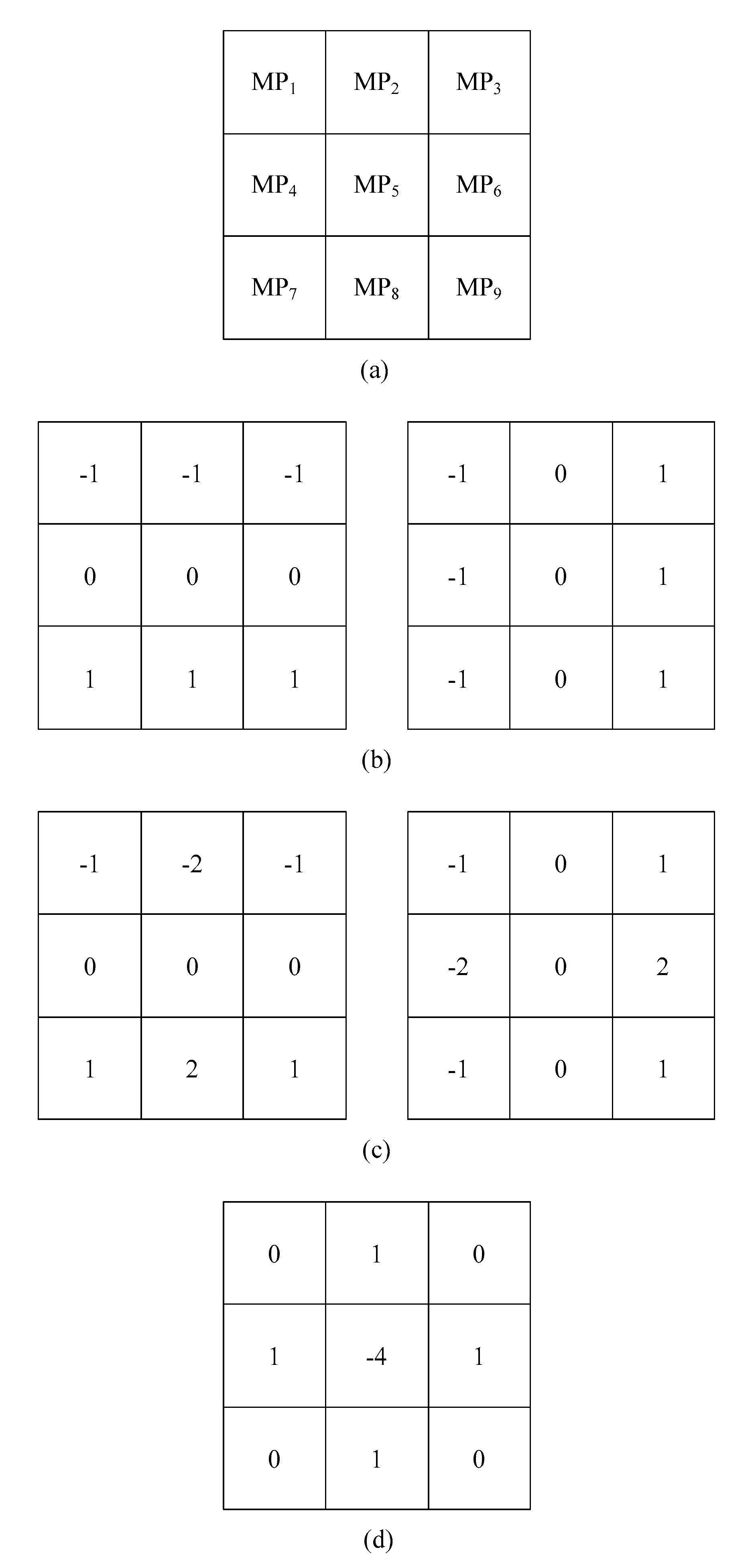
where M P is the central mixed pixel, and N M P is the neighborhood of the mixed pixel. P r e w i t t , S o b e l and L a p l a c i a n are the operations employing classic Prewitt, Sobel and Laplacian edge detection masks [19,26] and normalization, respectively. Figure 2a illustrates MP5, the mixed pixel and its neighborhood being investigated. Figure 2b,c and Figure 2d are the classic Prewitt, Sobel and Laplacian edge-detection masks, respectively [19,26].
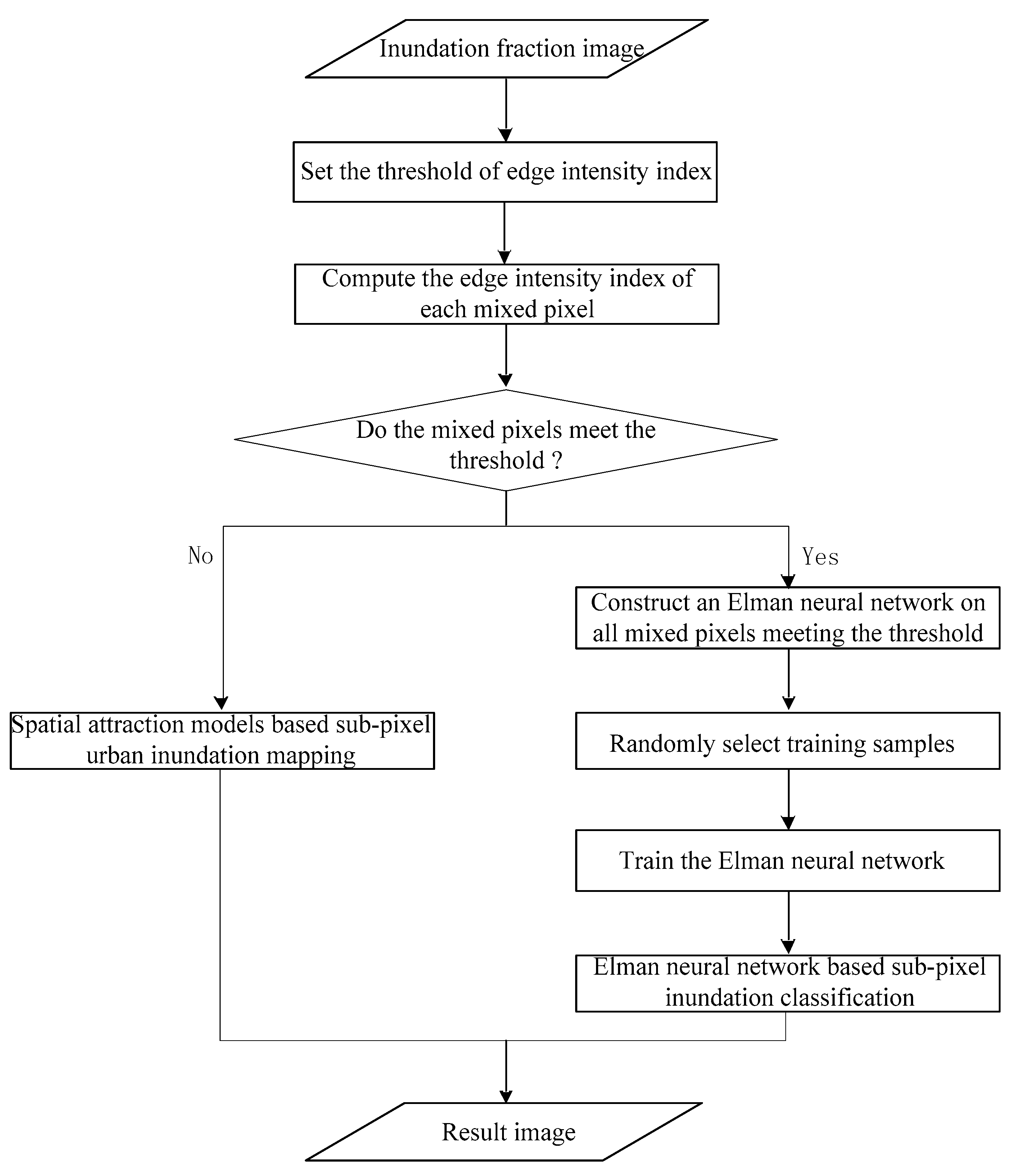
Due to high discontinuity of gray values, mixed pixels with highly curled edge are usually difficult for SUIM. However, they are also the key part of SUIM that has a potential to be better mapped in order to improve SUIM accuracy. In this study, NEII acts as a threshold to switch a current mixed pixel between two different processing models. If the NEII value of a mixed pixel is larger than a given threshold, SAMENN-SUIM constructs ENN-SUIM to acquire the spatial distributions of urban inundation at a sub-pixel scale. Otherwise, SAMENN-SUIM uses SAM to get the sub-pixel mapping results. Figure 3 shows the flow chart of SAMENN-SUIM.

3. Case Study

3.1. Experimental Results and Analysis

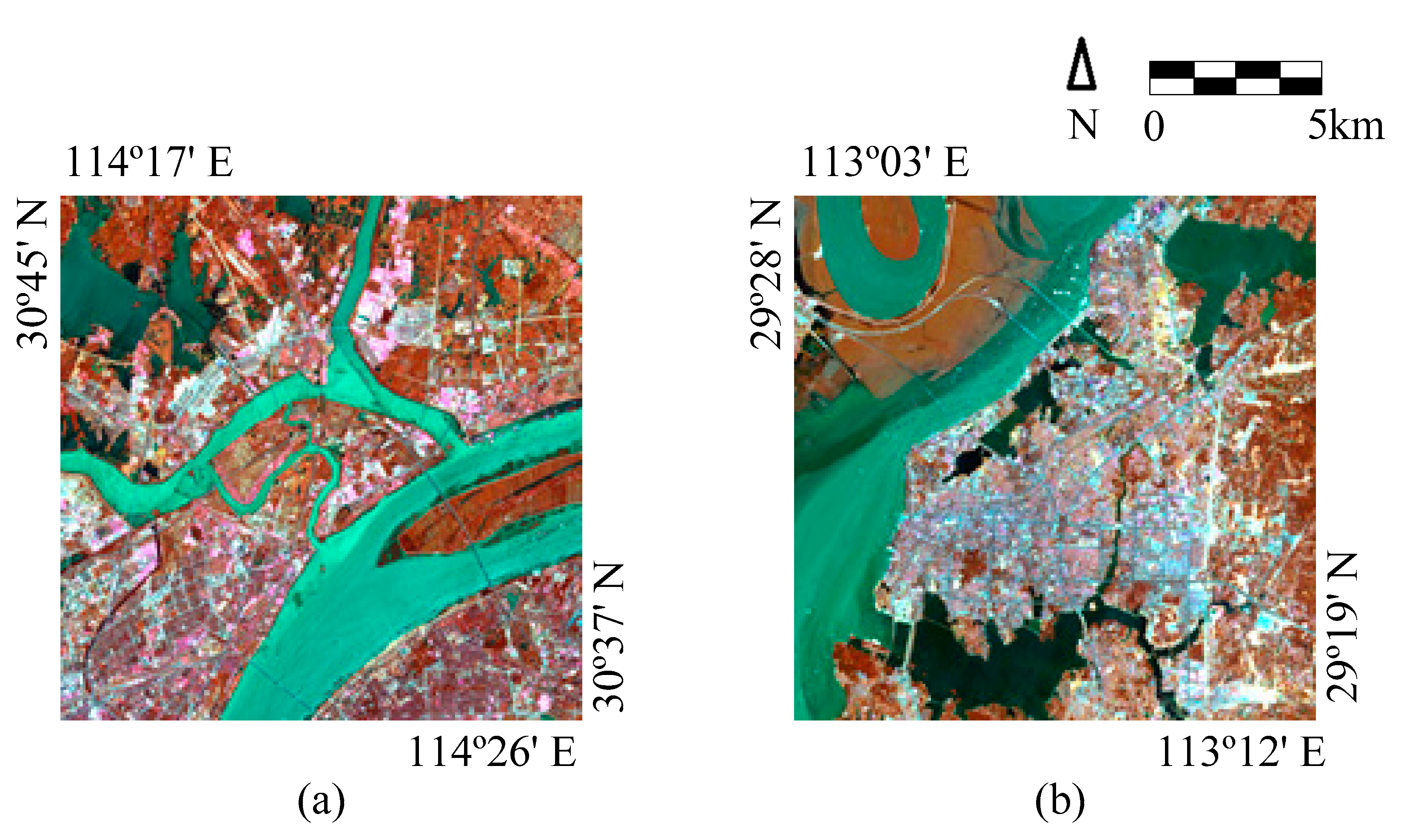
Severe floods struck Wuhan, Hubei Province, China in July, 2016 and Yueyang, Hunan Province, China in July, 2017, separately. Landsat 8 OLI multispectral images with 30 m resolution were used for experiments of this study. Representative study areas were selected and the image size of the study areas is 500 × 500 pixels. Figure 4 shows the two study areas.
Comparative SUIM methods chosen were back-propagation neural network-based SUIM (BPNN-SUIM), SVM-based SUIM (SVM-SUIM), SAM-based SUIM (SAM-SUIM) and SAMENN-SUIM. For BPNN-SUIM, SVM-SUIM and SAMENN-SUIM, we randomly chose 20% of the mixed pixels as the training samples. The number of the hidden layer was 1 and the neuron number of the hidden layer was 25 in BPNN-SUIM and SAMENN-SUIM. The NEII threshold was set at 0.1 in SAMENN-SUIM. The comparative algorithms and parameter values adopted are widely used in sub-pixel mapping and classification [12,16].
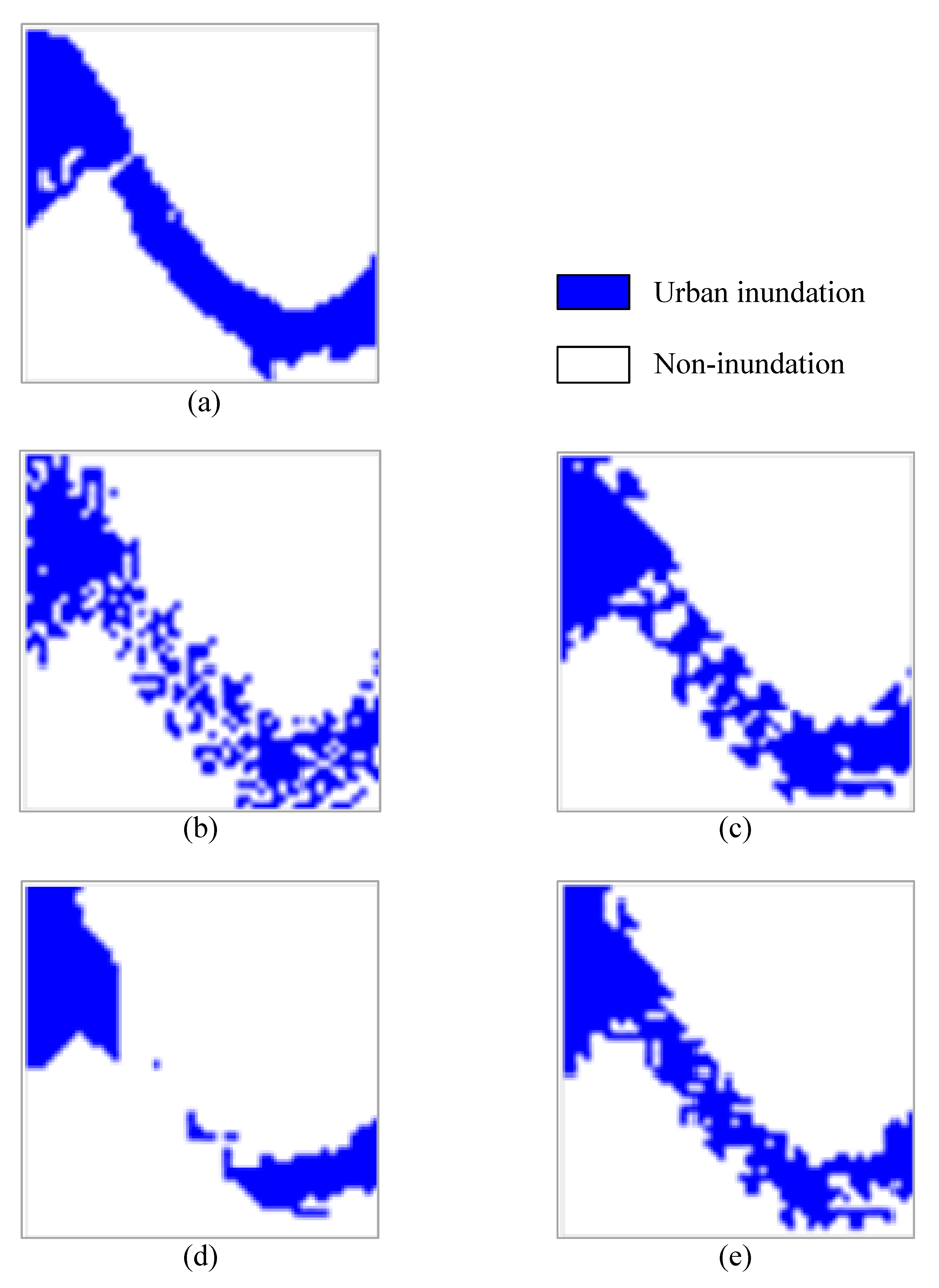
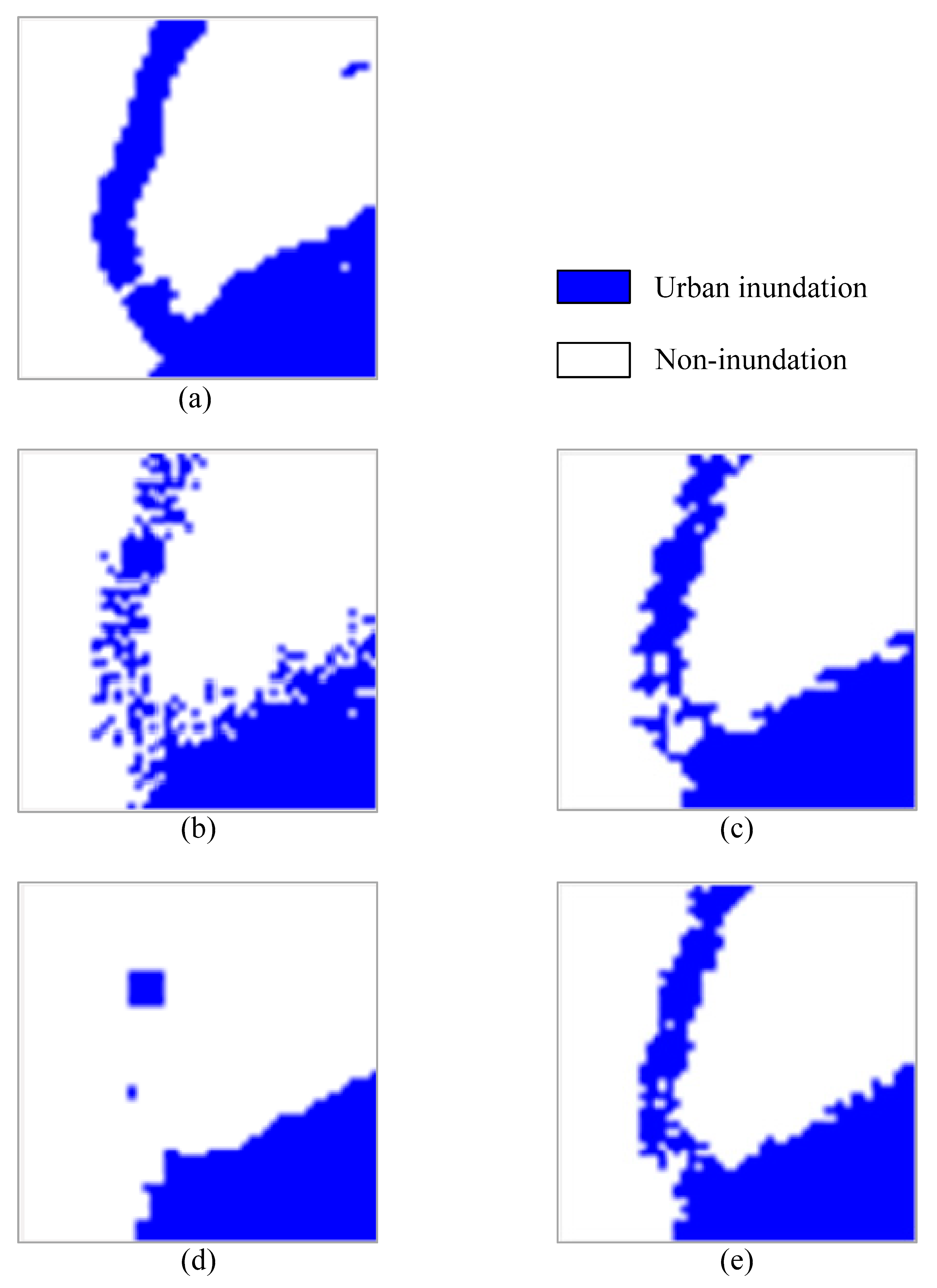
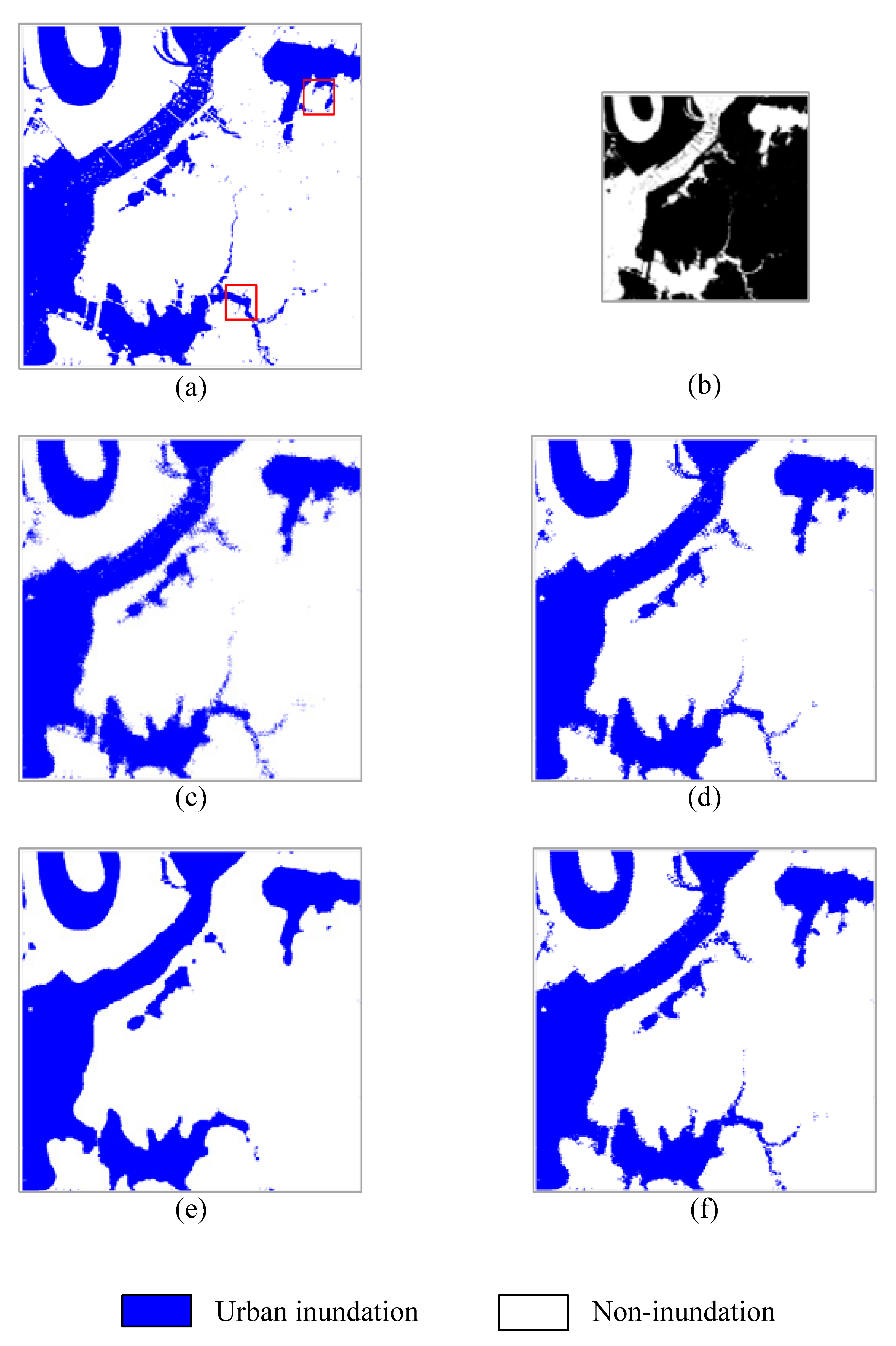
Figure 5 shows the experimental images and results of the four SUIM methods for Wuhan. The inundation reference image with 30 m resolution (Figure 5a) was acquired using the Landsat 8 multispectral image based on the modified normalized difference water index (mNDWI) [37,38,39,40]. The scale was set at 5 in the experiment. The inundation reference image was aggregated to get the inundation fraction image with 150 m resolution (Figure 5b), which was the input to the four SUIM methods. Figure 6 and Figure 7 illustrate zoomed small parts of the inundation reference image and the four SUIM results, which give a detailed comparison of those four methods. As shown in Figure 5, Figure 6 and Figure 7, SAMENN-SUIM has the best SUIM result for Wuhan city. Compared to other SUIM methods, SAMENN-SUIM maps urban flooding not only more continuously but also more smoothly. SAM is coupled with ENN in SAMENN-SUIM, which further boosts the performance of SUIM.
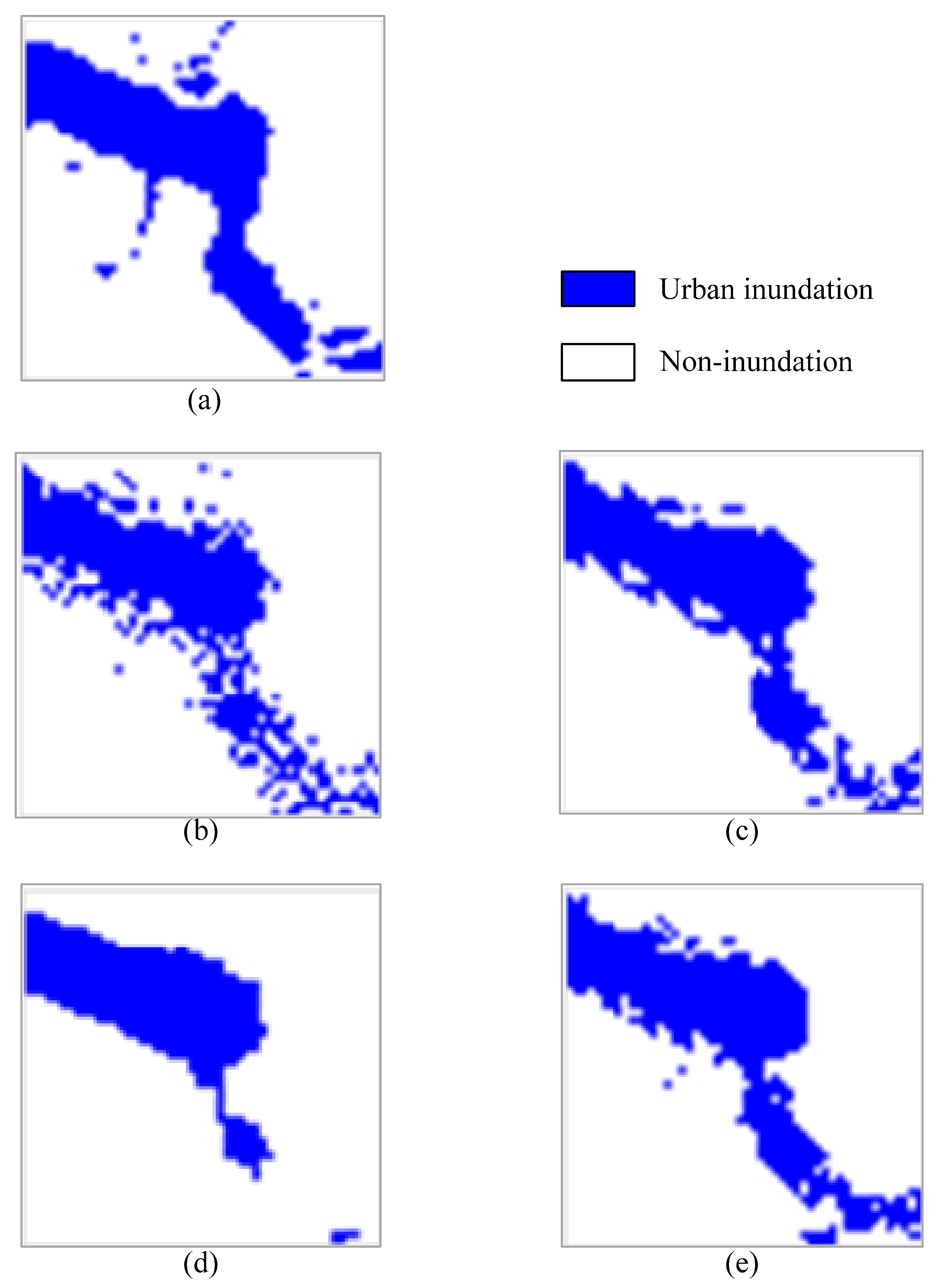
Figure 8 shows the experimental images and results of the four SUIM methods for Yueyang. Figure 9 and Figure 10 illustrate zoomed small parts of the inundation reference image and the four SUIM results, which give a detailed comparison of those four methods. From Figure 8, Figure 9 and Figure 10, it can be seen that SAMENN-SUIM gives the optimal SUIM result for Yueyang city as well.
Table 1 presents a quantitative evaluation of the four SUIM methods, measured using not only overall accuracy (OA) and Kappa coefficient (KC), but also average producer accuracy (APA) and average user accuracy (AUA) [41,42,43]. Only mixed pixels are included when computing the accuracy indices. SAMENN-SUIM attained the highest values of accuracy indices for the two cities. For instance, OA of BPNN-SUIM, SVM-SUIM, SAM-SUIM and SAMENN-SUIM are 72.9%, 78.9%, 78.3% and 80.1% for Wuhan, respectively. The OA of BPNN-SUIM, SVM-SUIM, SAM-SUIM and SAMENN-SUIM are 72.8%, 77.7%, 77.2% and 78.8% for Yueyang, respectively.

3.2. Summary

Urban floods have spatio-temporal distributions, so it is usually difficult to obtain the ground-truth data to validate the model. In order to apply and assess SAMENN-SUIM in real cases, two multispectral remote-sensing images are needed at the same time for a specific area, which are with different resolutions. One image is of a high resolution from which the flooding reference image is derived. Another image is of a low resolution from which the flooding fraction image is obtained. However, it is still difficult to obtain such valid images from two different satellite systems in the real case. If it is the case that these images are obtained, there will be no technical obstacles to apply the method. Take 4 m spatial resolution Gaofen-2 multispectral images and 30 m spatial resolution Landsat multispectral images, for example. First, a geometric registration is implemented on the two images. The resolution of the Landsat image is resampled to 28 m, which is seven times the resolution of the Gaofen-2 image. Second, a 2 8m flooding fraction image is derived from the Landsat image using the least squares linear spectral mixture analysis method [44]. Third, SAMENN-SUIM is applied to obtain a 4 m SUIM result from the 28 m fraction image. Finally, supervised classification methods are used to classify the Gaofen-2 image into a 4 m flooding reference image. The SUIM result is assessed using the visual and quantitative comparisons with the flooding reference image.

4. Discussion

4.1. Effects of Normalized Edge Intensity Index (NEII) Threshold in Spatial Attraction Models and Elman Neural Network Sub-Pixel Urban Inundation Mapping (SAMENN-SUIM)

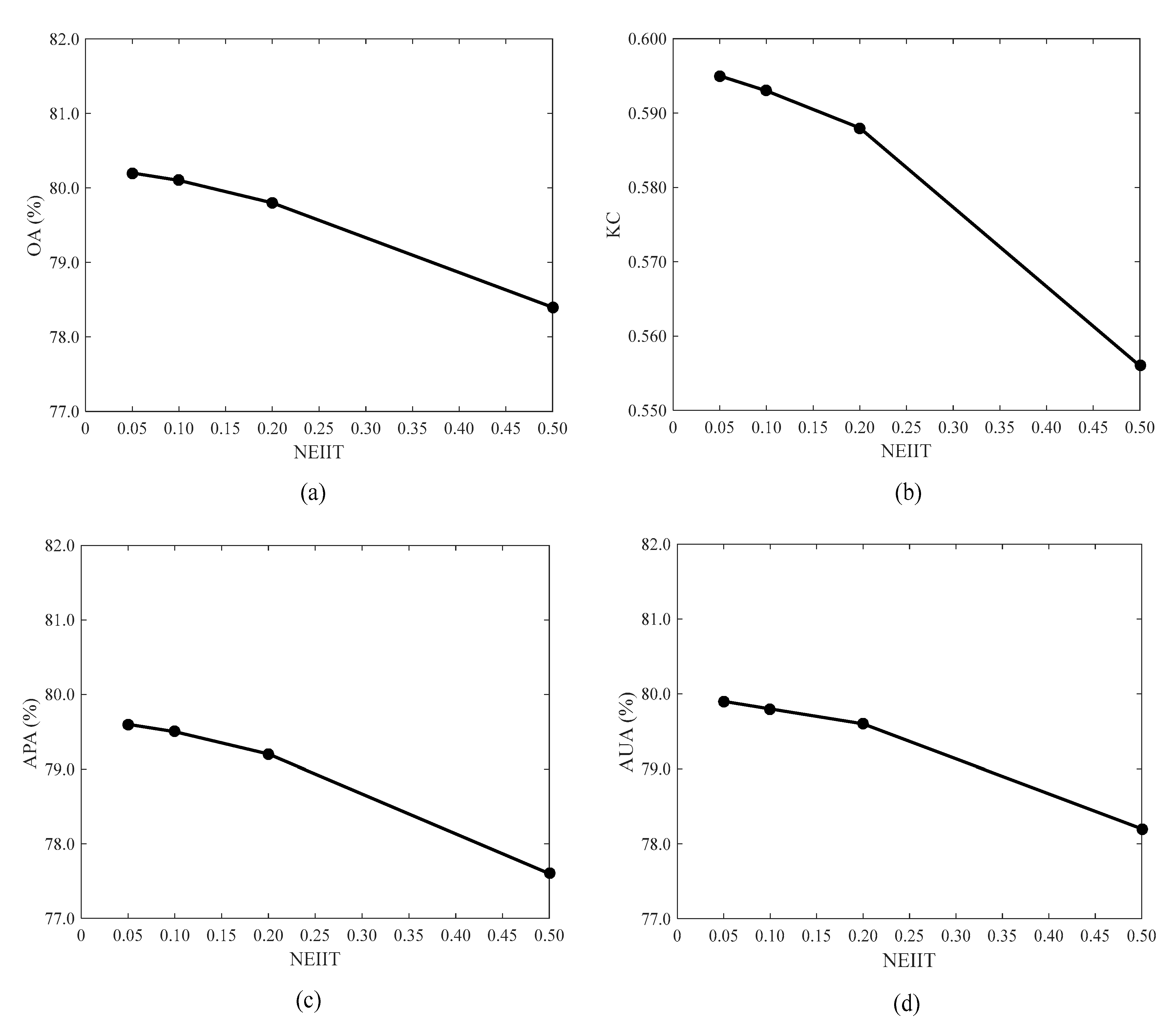
NEII acts as a threshold to direct a mixed pixel to a desirable processing model. In other words, the NEII threshold (NEIIT) decides the number of mixed pixels handled by ENN, which influences the accuracy of SAMENN-SUIM results. Accuracy of SAMENN-SUIM was investigated at four different NEIIT values for the Wuhan study area while keeping other parameters of SAMENN-SUIM unchanged, as shown in Figure 11. It can be seen that the larger the NEIIT, the smaller the OA. OA declines from 80.2% to 78.4% while NEIIT rises from 0.05 to 0.50. There is also a similar declining tendency in other accuracy indices, since a high NEIIT reduces the number of mixed pixels handled by ENN while raising the number of mixed pixels handled by SAM. While SAM has merits such as simplicity, ENN has a stronger capability to get better SUIM results when dealing with mixed pixels with an intricate edge.

4.2. Repeated Tests

Repeated tests were conducted to test the stability of SAMENN-SUIM using the Landsat 8 image for Wuhan. All the parameters of SAMENN-SUIM were the same as those in Section 3. Sub-pixel mapping results of SAMENN-SUIM in 20 repeated tests are shown in Table 2 where Min represents minimum value, Max represents maximum value, Mean represents mean value and SD represents standard deviation value. As can be seen from Table 2, the mean values of OA, KC, APA and AUA are 79.8%, 0.588, 79.3% and 79.6% for Wuhan, which are higher than the accuracy of the mapping results of three traditional methods in Section 3. Minimum values of OA, KC, APA and AUA are 79.6%, 0.582, 79.0% and 79.4%. Maximum values of OA, KC, APA and AUA are 80.1%, 0.593, 79.5% and 79.8%. Standard deviation values of OA, KC, APA and AUA are low, which are 0.135%, 0.003, 0.167% and 0.139%, Therefore, SAMENN-SUIM has good stability.

4.3. Effects of the Neuron Number of Hidden Layer in SAMENN-SUIM

Choosing the neuron number of a hidden layer is crucial to ENN, affecting the classification capability of ENN and hence affecting the accuracy of SAMENN-SUIM. Effects of the neuron number (NN) of the hidden layer in SAMENN-SUIM were investigated using the Landsat 8 image for Wuhan. Other parameters of SAMENN-SUIM were the same as those in the experiment. The effects of different neuron numbers of the hidden layer are shown in Table 3. Among the three NN values, the largest accuracy indices are acquired when NN value is equal to 25. The reason is that the higher the NN, the smoother the ENN’s function approximation, which is in favour of fitting the training samples closely and increasing the accuracy of sub-pixel mapping. However, if NN is too high, the ENN’s function approximation will over-fit training samples.

5. Conclusions

Urban flooding is one of the most costly and destructive natural hazards worldwide. A new algorithm called SAMENN-SUIM was developed to boost accuracy of urban inundation mapping in this study. After composing an ENN-based SUIM and choosing a proper normalized edge intensity of mixed pixels, the algorithm of SAMENN-SUIM was constructed, implemented and evaluated. Landsat 8 images of two cities of China, which experienced heavy floods, were used in the experiments. Compared to three traditional SUIM methods, SAMENN-SUIM obtained better mapping results according to not only visual evaluations but also quantitative assessments. OA values of BPNN-SUIM, SVM-SUIM, SAM-SUIM and SAMENN-SUIM are 72.9%, 78.9%, 78.3% and 80.1% for Wuhan, respectively. OA values of BPNN-SUIM, SVM-SUIM, SAM-SUIM and SAMENN-SUIM are 72.8%, 77.7%, 77.2% and 78.8% for Yueyang, respectively. The effects of the normalized edge intensity index threshold and the neuron number of hidden layer on the accuracy of SAMENN-SUIM were investigated and discussed. The novelty of this study is: (1) to develop the algorithm of ENN-SUIM; (2) to produce a normalized edge intensity index; and (3) to combine ENN with SAM for SUIM. Therefore, this study boosts urban inundation mapping accuracy from remote-sensing images with medium-low spatial resolutions, and hence can favor urban flood monitoring and risk assessment.

Author Contributions

Data curation, L.L., C.H. and K.S.; Methodology, L.L.; Supervision, Y.C., T.X. and L.M.; Writing—original draft, L.L. All authors have read and agreed to the published version of the manuscript.

Funding

This research was funded by [the National Key Research and Development Program of China] grant number [2018YFC0407804].

Conflicts of Interest

The authors declare no conflict of interest.

References

  1. Li, Y.; Martinis, S.; Wieland, M. Urban flood mapping with an active self-learning convolutional neural network based on TerraSAR-X intensity and interferometric coherence. ISPRS J. Photogramm. Remote Sens. 2019, 152, 178–191. [Google Scholar] [CrossRef]
  2. Bertilsson, L.; Wiklund, K.; Tebaldi, I.D.; Rezende, O.M.; Verol, A.P.; Miguez, M.G. Urban flood resilience—A multi-criteria index to integrate flood resilience into urban planning. J. Hydrol. 2019, 573, 970–982. [Google Scholar] [CrossRef]
  3. Tian, X.; ten Veldhuis, M.C.; Schleiss, M.; Bouwens, C.; van de Giesen, N. Critical rainfall thresholds for urban pluvial flooding inferred from citizen observations. Sci. Total Environ. 2019, 689, 258–268. [Google Scholar] [CrossRef] [PubMed]
  4. Farooq, M.; Shafique, M.; Khattak, M.S. Flood hazard assessment and mapping of River Swat using HEC-RAS 2D model and high-resolution 12-m TanDEM-X DEM (WorldDEM). Nat. Hazards 2019, 97, 477–492. [Google Scholar] [CrossRef]
  5. Percival, S.; Teeuw, R. A methodology for urban micro-scale coastal flood vulnerability and risk assessment and mapping. Nat. Hazards 2019, 97, 355–377. [Google Scholar] [CrossRef] [Green Version]
  6. Domeneghetti, A.; Schumann, G.J.P.; Tarpanelli, A. Preface: Remote sensing for flood mapping and monitoring of flood dynamics. Remote Sens. 2019, 11, 943. [Google Scholar] [CrossRef] [Green Version]
  7. Dou, X.; Song, J.; Wang, L.; Tang, B.; Xu, S.; Kong, F.; Jiang, X. Flood risk assessment and mapping based on a modified multi-parameter flood hazard index model in the Guanzhong Urban Area, China. Stoch. Environ. Res. Risk Assess. 2018, 32, 1131–1146. [Google Scholar] [CrossRef]
  8. Lin, L.; Di, L.; Tang, J.; Yu, E.; Zhang, C.; Rahman, M.S.; Shrestha, R.; Kang, L. Improvement and validation of NASA/MODIS NRT global flood mapping. Remote Sens. 2019, 11, 205. [Google Scholar] [CrossRef] [Green Version]
  9. Beaton, A.; Whaley, R.; Corston, K.; Kenny, F. Identifying historic river ice breakup timing using MODIS and Google Earth Engine in support of operational flood monitoring in Northern Ontario. Remote Sens. Environ. 2019, 224, 352–364. [Google Scholar] [CrossRef]
  10. Vichet, N.; Kawamura, K.; Trong, D.P.; On, N.V.; Gong, Z.; Lim, J.; Khom, S.; Bunly, C. MODIS-Based investigation of flood areas in Southern Cambodia from 2002–2013. Environments 2019, 6, 57. [Google Scholar] [CrossRef] [Green Version]
  11. Genitha, C.H.; Vani, K. A hybrid approach to super-resolution mapping of remotely sensed multi-spectral satellite images using genetic algorithm and Hopfield neural network. J. Indian Soc. Remote Sens. 2019, 47, 685–692. [Google Scholar] [CrossRef]
  12. Wang, P.; Zhang, G.; Hao, S.; Wang, L. Improving remote sensing image super-resolution mapping based on the spatial attraction model by utilizing the pansharpening technique. Remote Sens. 2019, 11, 247. [Google Scholar] [CrossRef] [Green Version]
  13. Wang, P.; Wu, Y.; Leung, H. Subpixel land cover mapping based on a new spatial attraction model with spatial-spectral information. Int. J. Remote Sens. 2019, 40, 6444–6463. [Google Scholar] [CrossRef]
  14. Li, X.; Li, X.; Foody, G.; Yang, X.; Zhang, Y.; Du, Y.; Ling, F. Optimal endmember-based super-resolution land cover mapping. IEEE Geosci. Remote Sens. Lett. 2019, 16, 1279–1283. [Google Scholar] [CrossRef]
  15. Xu, X.; Tong, X.; Plaza, A.; Li, J.; Zhong, Y.; Xie, H.; Zhang, L. A new spectral-spatial sub-pixel mapping model for remotely sensed hyperspectral imagery. IEEE Trans. Geosci. Remote Sens. 2018, 56, 6763–6778. [Google Scholar] [CrossRef]
  16. Li, L.; Chen, Y.; Xu, T.; Shi, K.; Huang, C.; Liu, R.; Lu, B.; Meng, L. Enhanced super-resolution mapping of urban floods based on the fusion of support vector machine and general regression neural network. IEEE Geosci. Remote Sens. Lett. 2019, 16, 1269–1273. [Google Scholar] [CrossRef]
  17. Su, Y. Integrating a scale-invariant feature of fractal geometry into the Hopfield neural network for super-resolution mapping. Int. J. Remote Sens. 2019, 40, 8933–8954. [Google Scholar] [CrossRef]
  18. Arun, P.V.; Herrmann, I.; Budhiraju, K.M.; Karnieli, A. Convolutional network architectures for super-resolution/sub-pixel mapping of drone-derived images. Pattern Recognit. 2019, 88, 431–446. [Google Scholar] [CrossRef]
  19. Gonzalez, R.C.; Woods, R.E. Digital Image Processing, 3rd ed.; Publishing House of Electronics Industry: Beijing, China, 2017; pp. 90–93. [Google Scholar]
  20. Zhang, Y.; Wang, X.; Tang, H. An improved Elman neural network with piecewise weighted gradient for time series prediction. Neurocomputing 2019, 359, 199–208. [Google Scholar] [CrossRef]
  21. Yang, L.; Wang, F.; Zhang, J.; Ren, W. Remaining useful life prediction of ultrasonic motor based on Elman neural network with improved particle swarm optimization. Measurement 2019, 143, 27–38. [Google Scholar] [CrossRef]
  22. Liu, H.; Xia, L.; Wang, C. Maneuvering target tracking using simultaneous optimization and feedback learning algorithm based on Elman neural network. Sensors 2019, 19, 1596. [Google Scholar] [CrossRef] [Green Version]
  23. Krishnan, S.; Lokesh, S.; Devi, M.R. An efficient Elman neural network classifier with cloud supported internet of things structure for health monitoring system. Comput. Netw. 2019, 151, 201–210. [Google Scholar] [CrossRef]
  24. Jia, W.; Zhao, D.; Zheng, Y.; Hou, S. A novel optimized GA-Elman neural network algorithm. Neural Comput. Appl. 2019, 31, 449–459. [Google Scholar] [CrossRef]
  25. Sun, X.; Gong, S.; Han, G.; Wang, M.; Jin, A. Pruning Elman neural network and its application in bolt defects classification. Int. J. Mach. Learn. Cybern. 2019, 10, 1847–1862. [Google Scholar] [CrossRef]
  26. The MathWorks, Inc. Available online: https://ww2.mathworks.cn/help/ (accessed on 12 June 2019).
  27. Lu, K.; Hong, C.; Xu, Q. Recurrent wavelet-based Elman neural network with modified gravitational search algorithm control for integrated offshore wind and wave power generation systems. Energy 2019, 170, 40–52. [Google Scholar] [CrossRef]
  28. Ruiz, L.G.B.; Rueda, R.; Cuellar, M.P.; Pegalajar, M.C. Energy consumption forecasting based on Elman neural networks with evolutive optimization. Expert Syst. Appl. 2018, 92, 380–389. [Google Scholar] [CrossRef]
  29. Lin, W.; Hong, C. A new Elman neural network-based control algorithm for adjustable-pitch variable-speed wind-energy Conversion Systems. IEEE Trans. Power Electron. 2011, 26, 473–481. [Google Scholar] [CrossRef]
  30. Huang, Y.; Wang, H.; Liu, H.; Liu, S. Elman neural network optimized by firefly algorithm for forecasting China’s carbon dioxide emissions. Syst. Sci. Control Eng. 2019, 7, 8–15. [Google Scholar] [CrossRef] [Green Version]
  31. Wan, X.; Yang, Q.; Jiang, P.; Zhong, P. A hybrid model for real-time probabilistic flood forecasting using Elman neural network with heterogeneity of error distributions. Water Resour. Manag. 2019, 33, 4027–4050. [Google Scholar] [CrossRef]
  32. Liang, Y.; Qiu, L.; Zhu, J.; Pan, J. A digester temperature prediction model based on the Elman neural network. Appl. Eng. Agric. 2017, 33, 143–148. [Google Scholar]
  33. Ghasemi, J.; Rasekhi, J. Traffic signal prediction using Elman neural network and particle swarm optimization. Int. J. Eng. 2016, 29, 1558–1564. [Google Scholar]
  34. Al-Dhafian, B.; Ahmad, I.; Hussain, M.; Imran, M. Improving the security in healthcare information system through Elman neural network based classifier. J. Med. Imaging Health Inform. 2017, 7, 1429–1435. [Google Scholar] [CrossRef]
  35. Wang, J.; Wang, J.; Fang, W.; Niu, H. Financial time series prediction using Elman recurrent random neural networks. Comput. Intell. Neurosci. 2016, 4742515. [Google Scholar] [CrossRef] [PubMed] [Green Version]
  36. NASA. Available online: https://www.nasa.gov/mission_pages/landsat/overview/index.html (accessed on 1 June 2020).
  37. Zhou, Y.; Dong, J.; Xiao, X.; Liu, R.; Zou, Z.; Zhao, G.; Ge, Q. Continuous monitoring of lake dynamics on the Mongolian Plateau using all available Landsat imagery and Google Earth Engine. Sci. Total Environ. 2019, 689, 366–380. [Google Scholar] [CrossRef]
  38. Roy, D.P.; Huang, H.; Boschetti, L.; Giglio, L.; Yan, L.; Zhang, H.H.; Li, Z. Landsat-8 and Sentinel-2 burned area mapping—A combined sensor multi-temporal change detection approach. Remote Sens. Environ. 2019, 231, 111254. [Google Scholar] [CrossRef]
  39. Song, Y.; Liu, F.; Ling, F.; Yue, L. Automatic semi-global artificial shoreline subpixel localization algorithm for landsat imagery. Remote Sens. 2019, 11, 1779. [Google Scholar] [CrossRef] [Green Version]
  40. Wang, X.; Xiao, X.; Zou, Z.; Hou, L.; Qin, Y.; Dong, J.; Doughty, R.B.; Chen, B.; Zhang, X.; Cheng, Y.; et al. Mapping coastal wetlands of China using time series Landsat images in 2018 and Google Earth Engine. ISPRS J. Photogramm. Remote Sens. 2020, 163, 312–326. [Google Scholar] [CrossRef] [PubMed]
  41. Stehman, S.V.; Foody, G.M. Key issues in rigorous accuracy assessment of land cover products. Remote Sens. Environ. 2019, 231, 111199. [Google Scholar] [CrossRef]
  42. Shi, L.; Ling, F.; Foody, G.; Chen, C.; Fang, S.; Li, X.; Zhang, Y.; Du, Y. Permanent disappearance and seasonal fluctuation of urban lake area in Wuhan, China monitored with long time series remotely sensed images from 1987 to 2016. Int. J. Remote Sens. 2019, 40, 8484–8505. [Google Scholar] [CrossRef]
  43. Rasanen, A.; Virtanen, T. Data and resolution requirements in mapping vegetation in spatially heterogeneous landscapes. Remote Sens. Environ. 2019, 230, 111207. [Google Scholar] [CrossRef]
  44. Heinz, D.C.; Chang, C. Fully constrained least squares linear spectral mixture analysis method for material quantification in hyperspectral imagery. IEEE Trans. Geosci. Remote Sens. 2001, 39, 529–545. [Google Scholar] [CrossRef] [Green Version]
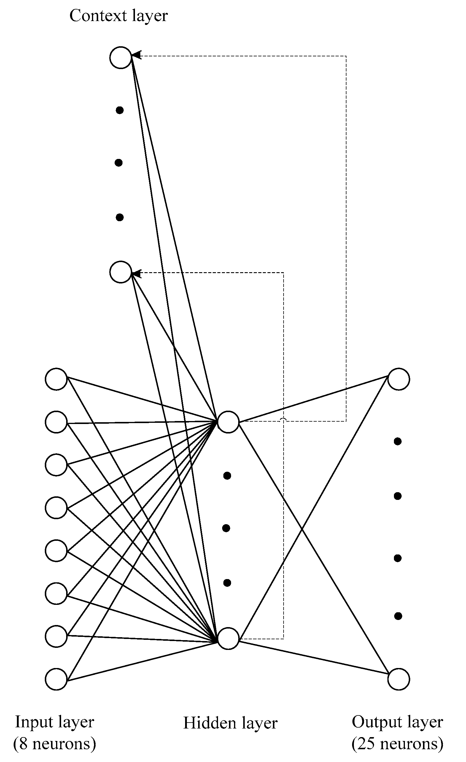
Figure 1. Elman neural network sub-pixel urban inundation mapping (ENN-SUIM) architecture (scale = 5).
Remotesensing 12 02068 g001
Figure 2. The neighborhood of the mixed pixel and classic edge detection masks. (a) The neighborhood of the mixed pixel; (b) Prewitt; (c) Sobel; (d) Laplacian edge detection masks.
Remotesensing 12 02068 g002
Figure 3. A flow chart of SAMENN-SUIM.
Remotesensing 12 02068 g003
Figure 4. Representative study areas. (a) Wuhan city; (b) Yueyang city.
Remotesensing 12 02068 g004
Figure 5. Experimental images and different SUIM results for Wuhan where red square shows the area for zooming. (a) Inundation reference image; (b) inundation fraction image; (c) back-propagation neural network (BPNN)-SUIM; (d) support vector machine (SVM)-SUIM; (e) spatial attraction model (SAM)-SUIM; (f) spatial attraction models and Elman neural networks (SAMENN)-SUIM.
Remotesensing 12 02068 g005
Figure 6. Zoom for small part 1 of inundation reference image and different SUIM results for Wuhan. (a) Inundation reference image; (b) BPNN-SUIM; (c) SVM-SUIM; (d) SAM-SUIM; (e) SAMENN-SUIM.
Remotesensing 12 02068 g006
Figure 7. Zoom for small part 2 of inundation reference image and different SUIM results for Wuhan. (a) Inundation reference image; (b) BPNN-SUIM; (c) SVM-SUIM; (d) SAM-SUIM; (e) SAMENN-SUIM.
Remotesensing 12 02068 g007
Figure 8. Experimental images and different SUIM results for Yueyang where red square shows the area for zooming. (a) Inundation reference image; (b) inundation fraction image; (c) BPNN-SUIM; (d) SVM-SUIM; (e) SAM-SUIM; (f) SAMENN-SUIM.
Remotesensing 12 02068 g008
Figure 9. Zoom for small part 1 of inundation reference image and different SUIM results for Yueyang. (a) Inundation reference image; (b) BPNN-SUIM; (c) SVM-SUIM; (d) SAM-SUIM; (e) SAMENN-SUIM.
Remotesensing 12 02068 g009
Figure 10. Zoom for small part 2 of inundation reference image and different SUIM results for Yueyang. (a) Inundation reference image; (b) BPNN-SUIM; (c) SVM-SUIM; (d) SAM-SUIM; (e) SAMENN-SUIM.
Remotesensing 12 02068 g010
Figure 11. Accuracy of SAMENN-SUIM relating to normalized edge intensity index threshold (NEIIT) for Wuhan. (a) OA in relation to NEIIT. (b) KC in relation to NEIIT. (c) APA in relation to NEIIT. (d) AUA in relation to NEIIT.
Remotesensing 12 02068 g011
Table 1. Quantitative evaluation of the four SUIM methods.
MethodsWuhanYueyang
OA (%)KCAPA (%)AUA (%)OA (%)KCAPA (%)AUA (%)
BPNN-SUIM72.90.44672.272.572.80.45572.772.9
SVM-SUIM78.90.57278.778.577.70.55377.677.7
SAM-SUIM78.30.55377.378.277.20.54377.177.5
SAMENN-SUIM80.10.59379.579.878.80.57678.878.8
Note: OA represents overall accuracy, KC represents Kappa coefficient, APA represents average producer accuracy and AUA represents average user accuracy, respectively.
Table 2. Twenty repeated tests of SAMENN-SUIM for Wuhan.
TestOA (%)KCAPA (%)AUA (%)
179.70.58679.279.4
579.90.58879.379.6
1079.60.58279.079.4
2080.00.59079.479.7
Min79.60.58279.079.4
Max80.10.59379.579.8
Mean79.80.58879.379.6
SD0.1350.0030.1670.139
Table 3. Effects of the neuron number (NN) of hidden layer in SAMENN-SUIM for Wuhan.
NNOA (%)KCAPA (%)AUA (%)
579.70.58679.279.4
2580.10.59379.579.8
5079.90.58979.379.6