Abstract
Knowledge of the free draft of ports is essential for the adequate management of ports. To maintain these drafts, it is necessary to carry out dredging periodically, and to conduct bathymetries using traditional techniques, such as echo sounding. However, an echo sounder is very expensive and its accuracy is subject to weather conditions. Thus, the use of recent advancements in remote sensing techniques provide a better solution for mapping and estimating the evolution of the seabed in these areas. This paper presents a cost-effective and practical method for estimating satellite-derived bathymetry for highly polluted and turbid waters at two different ports in the cities of Luarca and Candás in the Principality of Asturias (Spain). The method involves the use of the support vector machine (SVM) technique and open Sentinel-2 satellite imagery, which the European Space Agency has supplied. Models were compared to the bathymetries that were obtained from the in situ data collected by a single beam echo sounder that the Port Service of the Principality of Asturias provided. The most accurate values of the training and testing dataset in Candás, were R2 = 0.911 and RMSE = 0.3694 m, and R2 = 0.8553 and RMSE = 0.4370 m, respectively. The accuracies of the training and testing dataset values in Luarca were R2 = 0.976 and RMSE = 0.4409 m, and R2 = 0.9731 and RMSE = 0.4640 m, respectively. The regression analysis results of the training and testing dataset were consistent. The approaches that have been developed in this work may be included in the monitoring of future dredging activities in ports, especially where the water is polluted, muddy and highly turbid.
1. Introduction
A bathymetric model is an essential source of information for an understanding of the marine environment. It should be the starting point for any project that is based on marine cartography. Accurate bathymetry data also facilitate the habitat assessment [1,2], classification and detailed representation of the seabed [3] and an understanding of the morphology of the area. Water depth information is also essential for hydrodynamic and wave modelling, sediment transport and environmental exploration, facilitates simulation of the impact of construction and dredging activities, etc. [4]. Similarly, accurate bathymetry data are of utmost importance for the stabilization of beaches and, hence, the security of buildings that are located near the sea. Further, it is essential in scientific research and modeling sea floor relief. These are also necessary for the exploration, exploitation, conservation and administration of natural resources and, especially, for a coastal environment impact assessment and protection. [5,6].
The ports are viewed as buffer zones or protected areas, in which ships can find protection from the action of waves. These configurations of the ports aid the dissipation of the waves, but not the action of the coastal dynamics. The coastal dynamics mobilize the sediments, which are then deposited in the calm water areas of the ports. Consequently, dredging operations are required to empty the navigation channel of these sediments and avoid serious disaster [7]. Dredging recovers the seabed that is currently full of sand and thus facilitates access by ships to the ports by means of the navigation channel. Dredging is also required to ensure that the minimum draft that is necessary for ships to navigate and maneuver within the ports is maintained. It is also necessary for the development of port infrastructure. Bathymetric mapping is used in, and is essential to, the management of such port operations. In any event, whether bathymetric work is used as an aid to navigation or as part of a process or activity in maritime engineering, its high economic significance is clear. Even small variations in vertical measurement would have great economic repercussions if the level of error if not evaluated. However, on some occasions, knowledge of errors is necessary. On other occasions, it is helpful to reduce any errors and, therefore, increase the reliability of the information. Bathymetry studies are conducted by the use of various techniques. Each technique can give a different result depending on the precision that it provides. Conventional techniques, such as airborne-, ground- and ship-borne-based surveying provide very accurate measurements [8]. Among the most commonly used techniques is the use of echo sounders. Techniques that involve vessel-based single beam echo sounding, however, are limited due to problems in accuracy and precision, as well as the difficulty to access shallow coastal waters. Currently, multibeam echo sounders and light detection and ranging (LiDAR) are commonly used for high-resolution bathymetry retrieval in shallow areas [9,10]. Nevertheless, these techniques are better employed in small areas and are limited by high costs [8,9,10,11,12]. These factors cause other techniques, such as remote sensing, to become competitive and attractive methods of providing reliable depth estimates at a much lower cost [13,14].
Remotely sensed technology is considered a low-cost, time-effective and widely adopted solution for satellite-derived bathymetry (SDB), which can be considered as a promising alternative tool to map bottom depths in areas with highly dynamic seabed characteristics [15]. SDB methods can be classified according to a physics-based approach or empirical approach: the first simulates the light that interacts through the water column, and the second develops regressions between spectral radiation and in situ calibration data [16]. Bathymetric information from shallow areas is key to managing coastal environments, however, there is still incomplete and spatially limited coverage, especially in optically shallow areas because the water clarity has a significant and variable impact on SDB accuracy.
Machine learning methods have been used to estimate water depth from remote optical images. One of the initial attempts used a combination of multispectral data and radiometric techniques [17]. With the arrival of Landsat images, bathymetry monitoring methods were improved and applied effectively to optical satellite images [18,19]. The advancement of remote sensing technology has enabled numerous researchers to expand the use of these techniques with improved spectral resolution [20,21,22]. In recent years, thanks to the technological advances and improvements that satellites are bringing to the study of the marine environment, topographic surveys are conducted by the use of satellites and remote sensing technology. This technology permits the use of high-resolution satellite images to determine depth ranges based on the wavelength of the spectral bands of the image. The main obstacles that are encountered when applying these technologies are the turbidity of the water and the reflectance penetration [23]. The suspended particulate matter, which is the main contributor to turbidity, introduces a confusing reflectance of light that the satellite detects. The waters of different turbidity levels disperse the incoming radiation differently, which implies greater complexity and development problems in the highly dynamic coastal regions and anthropogenic ecosystems of the ports [24,25].
In this study, regular optical satellite images were used. More specifically, the ESA Sentinel-2 constellation (two satellites) was used to obtain bathymetric mapping by the use of a support vector machine (SVM), a machine learning technique. These satellites’ images are freely available, have a resolution of 10 to 60 m and a revisit interval of five days. Sentinel-2 has six land monitoring bands, each of which can be compared to Landsat-8. In addition, the satellite has three other bands, thereby covering the red-edge spectrum [26]. At present, these data that this satellite provides and the use of advanced computational techniques for bathymetry estimations represent an important advancement in this field [27,28,29].
To obtain deep water inversion from optical sensors, investigators have employed regression models that are based on machine learning techniques. Liu et al. [30], for example, investigated the performance of two artificial neural network methods—general regression neural networks (GRNN) and multilayer perceptron (MLP)—as methods for possible use in bathymetry studies. The results showed that artificial neural networks are more useful and accurate than the inversion model and regression tree. Other researchers have used an artificial neural network (ANN) [31,32] for estimating the depths of shallow waters. More recently, other authors used the machine learning technique of SVM to estimate shallow water depths, for instance, [25] applied the non-linear machine learning technique of SVM to Landsat images in Saint Maarten Island and the Ameland Inlet in the Dutch Wadden Sea and experienced an overall error of 8.26% and 14.43%, respectively. At Kauai Island in Hawaii, [33] proposed a spatially distributed SVM system to use in estimating the bathymetry of shallow water by the use of optical satellite images, as well as SVMs that were locally trained with spatially weighted votes for the prediction. In the present case, the experimental results indicated that the localized model gave a 60% lower bathymetry estimation error than from the root mean squared error (RMSE). In recent years, with the use of remote optical observation, many studies have been undertaken to estimate bathymetry in shallow water [25,34]. However, because the underlying surfaces of the harbors are submerged and frequently obscured by turbid and mud, it can be difficult to estimate changes in depths of the bottoms of harbors. Only recently, on the coast of Misano, Muzirafuti et al. [35] published a comparative quantitative analysis of the log band ratio and the optimal band ratio methods of analysis, which are employed regularly in bathymetry. The study considered the potential application of these methods in the multispectral satellite imaging of a coastal area to determine the spectral band ratio that would provide water depth information with the most accuracy, particularly in shallow turbid water. This methodology implies having great knowledge of data processing. A simple system is sought in this work in order to apply it to the management of ports without a need to resort to the bathymetry conducted in situ using an echo sounder.
This study presents optimal satellite-based bathymetry derivation models that have been developed for use with highly turbid waters at two different ports in the cities of Luarca and Candás in the Principality of Asturias (Spain). The research used data that were provided by the Sentinel-2 satellite, as well as the logarithmic relationship and analytical approaches using SVM. The work has sought to provide an efficient method to derive bathymetric data from Sentinel-2 images. Satellite-derived bathymetry maps can be used to provide low-cost and high-density data for later use in numerical models in port research. It is hoped that the approach that was developed in this work is included in the monitoring of the bathymetry of the Candás and Luarca ports as a fast and economical alternative to conventional bathymetry to evaluate the need for dredging. This technique can be used also in studying coastal management.
2. Materials and Methods
2.1. Study Sites and Data Sites
The first study site is the port of Candás (Figure 1). Candás is a coastal town in Asturias Principality in one of the northernmost points of the Iberian Peninsula. The town has a population of approximately 7000 inhabitants. Candás has a medium-sized port where fishing boats and nautical sports boats coexist, although the latter outnumber the former. The port has 188 fixed moorings and 48 temporary moorings for use by nautical sports boats. The minimum drafts of the port range between 3.5 m in the navigation channel and 1 m at the interior docks, where the boats are small. Fish production in 2019 was 112 tons.
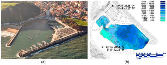
Figure 1.
Study area (a) Candás port; (b) bathymetry using echo-sounding measurements. The colors denote the depth of the water in meters.
Bathymetric data were obtained from the Port Service of the Principality of Asturias, which conducts accurate bathymetric studies that concern modeling water quality and morphological changes in ports. These bathymetries are conducted to ensure good management of the exploitation of the ports. Knowledge of the seabed facilitates the appropriate management and exploitation of the ports. Therefore, the bathymetric studies are conducted as part of its conservation and maintenance work for the planning of dredging. In this study, the only three available bathymetric charts for 2016, 2018 and 2019 were used to adjust the satellite images at various depths. This bathymetric information was collected by use of an echo sounder single beam Navisound 210 (Reson, Inc.; Slangerup, Denmark) that has a variable frequency acoustic profiler (201 kHz/33 kHz). Its position was determined by using GPS. The second study site was Luarca port (Figure 2), a coastal town in the western area of the Principality of Asturias in Spain. The town has a population of approximately 5200 inhabitants. It has a medium-sized port that is home to fishing boats and nautical sports, although the fishing sector predominates. Fish production in 2019 was 499t. As the boats that use the port are generally small vessels, the minimum drafts range between three meters in the navigation canal and two meters in the docking area. Bathymetric data also were collected by use of an echo sounder single beam Navisound 210 dual frequency (190–235 kHz), and a 1 cm vertical resolution.
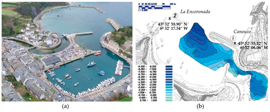
Figure 2.
Study area (a) Luarca port; (b) bathymetry using echo-sounding measurements. The colors denote the depth of the water in meters, and the number denotes the dikes of Canouco and La Encoronada.
The study’s echo sounding data for this area were determined by reference to survey positions of the UTM/WGS84 ZONA 30N, on 16 October 2016, 12 March 2018 and 29 April 2019 in the case of Candás, as well as 28 June 2016, 10 May 2018 and 28 May 2019 for Luarca (see Table 1). The port data points for the in situ measurements at Candás were taken by several passes of the vessel. The distribution of the passes was made using a 10 × 20 m mesh. In Luarca, the data points were taken by passes, the distribution of which was made with a 10 × 30 m mesh in the sheltered area (between the Canouco and La Encoronada dikes, see Figure 2b) and 30 × 30 m in external waters.

Table 1.
Dates of acquisition of Sentinel-2 data and in situ measurements data.
2.2. Satellite Data
The data from the Sentinel-2A and -2B twin polar-orbiting satellites were used to estimate the study sites’ depth of water. Sentinel-2 imagery data can be obtained from the European Space Agency’s sci-hub-portal (ESA) [36,37]. The satellites Sentinel-2A and -2B were launched on June 23, 2015, and March 2017, respectively [38]. In order to evaluate the capabilities of Sentinel-2′s coastal capabilities, it is necessary to possess a thorough understanding of revisit intervals and statistics regarding the world’s coastlines. Sentinel-2 collects data during its orbital ground swaths. These data are subsequently interpolated on military grid reference system (MGRS) zones that can be accessed by the public. The Sentinel-2 images were collected on 3 November 2016, 16 March 2018 and 22 April 2019 in Candás port. In the study of Luarca, the satellite images were collected on 29 June 2016, 10 May 2018 and 30 May 2019 (see Table 1). The Sentinel-2 satellite is equipped with a single multispectral instrument (MSI) that has thirteen spectral bands. The bands use a push broom sensor. The latter collects rows of image data during the orbital swath and uses the satellite’s forward motion along its path to generate new rows for acquisition [39]. Bands have a spatial resolution of 10 to 60 m. For example, the resolution of B2, B3, B4 and B8 is 10 m, whereas that of B5, B6, B7, B8A, B11 and B12 is 20 m. The resolution of the remaining bands is 60 m (Table 2). The dataset from Sentinel-2 was chosen due to its temporal proximity to the echo-sounding bathymetry dates and the availability of cloud free data.
Table 2.
Sentinel-2 bands.
2.3. Methodology
2.3.1. Pre-Processing of Satellite Images
The Sentinels Application Platform (SNAP) was used to view and export data. It is software offered at no charge by the European Space Agency [37] to process and analyze satellite images from the Sentinel satellite fleet. This program has a repertoire of tools (called Sentinel Toolboxes) that are specific to working with the images, whether they are Sentinel-1 radar images or the optical Sentinel-2 and Sentinel-3 multiband images. In any case, the SNAP tools can be used to manage multispectral images from missions, such as Envisat, Landsat, MODIS or SPOT. What was obtained were data from bands with different resolutions. The first step in using these data is to transform all bands to the same resolution. All spectral bands of the Sentinel-2 image were resampled to a 10 m resolution [40,41]. Resampling of the downloaded images was conducted with the software ESA SNAP (v7.0.1) [42] using the S2 Resampling Processor. As a result, a set of data is obtained that is not georeferenced, because we have only the longitude and latitude of the corners of the study portion. To determine the positioning of the reference points, the geographical location of each point is defined by its longitude and latitude using the SNAP program. From the longitude and latitude, a coordinate projection is made using the WGS84 ellipsoid, obtaining the coordinates in ETRS89. This is the same system with which the positions obtained by the echo sounder are projected. Position average errors in the ellipsoid projections are of the order of 1 cm.
2.3.2. Pre-Processing of Data. Generation of Comparison Bathymetry Grid
The data obtained were compared to the bathymetry projected. For this, coordinates were projected using a geodetic calculator, since the bathymetry uses ETRS89 coordinates, based on the same ellipsoid WGS84. Then, the data of the bands that are associated with UTM x-y coordinates could be obtained. To assign the z coordinate, the annual bathymetries of the study ports are used. These are undertaken by a single beam probe that is mounted on a vessel. From these z data that are obtained every 10 cm, a surface of the port’s bottom is generated. This surface is obtained using digital models of the terrain type triangulated irregular network (TIN). In this case, triangulation is conducted using linear interpolation. The error generated in this process is small since the surfaces of the seabed are smooth surfaces and without great irregularities. The z coordinates are referenced to zero of the port itself (the minimum level that has been measured at the highest low tide of the last 15 years). Each pixel is assigned the corresponding dimensions based on the former’s x-y location (Figure 3).
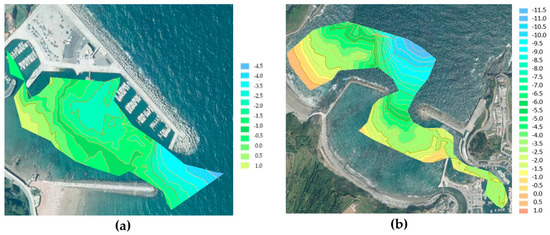
Figure 3.
Bathymetry maps obtained using echo sounder in situ measurements. (a) Candás; (b) Luarca. The colors denote the depth of the water in meters.
2.3.3. Bathymetry Estimation Based on Support Vector Machines
This study applied support vector algorithms to derive bathymetry from water reflectivity. Stumpf et al. [43] suggested a linear model, despite the fact that, in many ways, it did not always result in a relationship between the water depths and the ratio that was linear. Thus, it is best to obtain it by exploring the relationship of a non-linear function (f) to map water depth (Z) (Equation (1)).
where n is a fixed value and Rw is the reflectance that has been observed for the wavelength (λ) of bands i and j.
Support vector machine is one of the many non-linear regression techniques. It has been studied extensively and finds use as a universal approximation [44,45,46]. SVM has some advantages over other methods. Its classification accuracy is relatively higher when the inputs are correctly selected. This method is based on a kernel-based algorithm. Its new input estimations depend on an evaluation by the kernel function of a subcategory of events in a training stage. The task to use this method is to identify a function that will minimize Equation (2)’s final error.
where y(x) is the predicted value, b represents the value of the bias and ϕ(x) maintains the feature space transformation. An insensitive error function (Equation (4)) replaces the error function in the linear regression (Equation (3)) in this method. Equation (4) assigns a zero to values if is greater than the difference between the predicted and target value. If the difference is greater than, or equal to , the value of the error function does not change. To minimize Equation (5), the difference between the predicted and targeted values is also assigned a cost (C).
where y(x) is the value that is predicted by Equation (2), t denotes the searched target function, ϵ is the margin when the function fails to penalize and C denotes the penalty. The process is optimized, although the initial function (Equation (3)) becomes more complex (Equation (6)).
where α is one solution to the optimization problem that can occur with the Lagrangian theory. The data are changed by the function to data of a feature space. This improves the non-linear problem’s accuracy. As a result, the final function resembles Equation (7).
For the purpose of classification, the best kernel is generally the Gaussian radial basis function (RBF). It provides the greatest overall accuracy and kappa [47]. This study used this RBF function (Equation (8)).
To program the methodology that was proposed, the R statistical software was selected [48].
2.3.4. Data Processing
In this work, the dataset was used for the support vector machine studies in the two study areas of Candás and Luarca. Model training used 80% of the data points and testing accounted for the remaining 20% (Table 3). This ratio is common in machine learning studies [49,50]. The tests were conducted with several random data segmentations a total of 20 times. The additional results were eliminated and the average of the remaining data was used for the studies.
Table 3.
Number of data points of the training and testing data sets for the study areas.
Checking and applying a valid methodology is necessary for the implementation of the remote sensing measurements of the bathymetry of a specific area from optical images. In doing so, it was necessary to discriminate and select only the most appropriate bands and to determine the corrections of the images. The input variables that were used to model the bathymetry using SVM techniques were correlated using Equation (1). If all possible combinations between bands were considered, the number of input variables would be 68. Considering that this number of input variables was excessive, and in order to optimize them, the correlation of the different bands to each other was analyzed. To conduct the correlation analysis of the various bands, Pearson’s correlation coefficient was used. Pearson’s correlation coefficient (R) appears in Table 4 as a measure of the linear correlation of each study’s corresponding band pairs. A 1.0 coefficient of correlation indicates that two variables are correlated perfectly, whereas a coefficient of 0.0 indicates the absence of a linear relationship [51]. Most bands, except B9 and B1, were highly correlated with each other. To determine which bands were unnecessary, the pairs of bands that had a correlation greater than 0.9 were plotted. Figure 4 provides the scatter diagrams that show the relationship between pairs of bands that seem to supply visually the same information from Sentinel-2. Perfect agreement between two bands was indicated in each diagram by a 1-to-1 line.
Table 4.
R values between main bands of Sentinel-2.
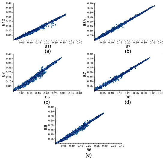
Figure 4.
Scatter diagram of the relationship of the pairs of bands that appear to provide visually the same information from Sentinel-2.A (a) B11-B12; (b) B7-B8A; (c) B5-B7; (d) B7-B6; (e) B5-B6.
Figure 4 indicates the high correlation between the bands. For this reason, some of the bands represented (B5, B6, B8A and B11) were eliminated for modeling with SVM. Under the same conditions, the bands with the highest resolution were maintained, since they have no calculated data due to interpolation. Subsequently, the correlation of these 28 variables was analyzed again, and one variable was eliminated. The bands that were chosen for data modeling were B1, B2, B3, B4, B7, B8, B9 and B12. Finally, the status of the tide at the time of the orthophoto was added as an input variable to the model.
3. Results and Discussion
A comparison was made of the bathymetry that the Sentinel-2 satellite data made possible and what the echo sounder in situ measurements provided for the ports of Candás and Luarca. The mean absolute error (MAE) and the root mean squared error (RMSE) were analyzed to determine the generalization capacities of the regression models. They can be calculated by equations 9 and 10.
In this case, ZSVM is the SVM predicted depths from Sentinel-2 images and Zecho is the echo sounder depths from the field data points. Further, the coefficient of determination is provided, it (R2) indicates the regression model’s “goodness of fit.” On the other hand, the adjusted R2 penalizes the R2 value for each predictor variable in the regression model (in this case, the input variable).
Table 5 shows the depth characteristics of the study areas. It shows negative values for the minimum depth (−5.0149 m in Candás and −11.9601 m in Luarca). The reason for this is that zero, “0”, refers to the minimum level that has been registered in that port. In Spain, Royal Decree 1071/2007 established that the surface of the sea in the city of Alicante (Spain) has a zero value. Therefore, a bathymetric measurement is normally considered to be the distance between the bottom to the zero value, zero. In this study, it is considered to be the lowest value of the surface of the water at each port (i.e., the minimum level that has been measured at the highest tide in the last 15 years).
Table 5.
Depth characteristics of the study areas.
The coefficient of determination or R2, MAE and RMSE that appear in Table 6 were obtained to determine the ability to predict and generalize of the SVM regression model that was obtained using the training dataset. It can be seen that the values of both R2 coefficients for Candás (R2 = 0.911) and Luarca (R2 = 0.976) are very close to 1, which is high. This indicates a high correlation between the observed and estimated values. The table also shows that the MAE and RMSE values are small and similar for Candás (MAE = 0.2779 m and RMSE = 0.3274 m) and Luarca (MAE = 0.3694 m and RMSE = 0.4409). Thus, the adjustment of the regression model is accurate.
Table 6.
Results for R2, mean absolute error (MAE), root mean squared error (RMSE) and relative error in a comparison of support vector machine (SVM) predicted values and in situ measurement values of depths using the training dataset.
After determining the R2, MAE and RMSE errors, scatter diagrams of the SVM predicted depth from the Sentinel-2 images (ZSVM) vs. the echo sounder depth (Zecho) from the training dataset for Candás (see Figure 5) and Luarca (see Figure 6) were created. The points that are closest to the diagonal line have the highest correlation to the regression models. In this case, both the Candás and Luarca training dataset points are very close to the diagonal line.
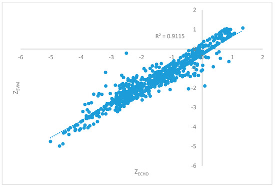
Figure 5.
Scatter diagram of training data showing SVM predicted depth (m) from Sentinel-2 images (ZSVM) vs. echo sounder depth (Zecho) from field data points for Candás.
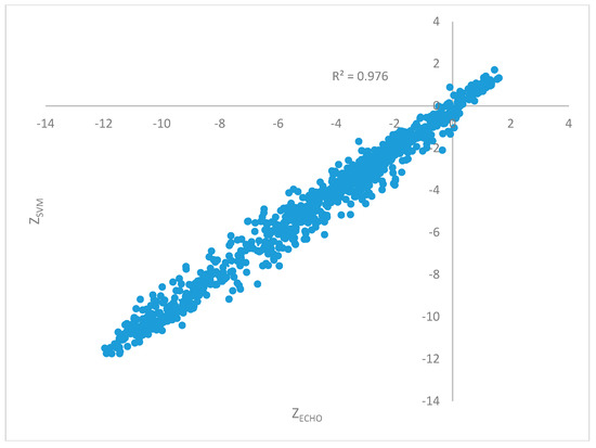
Figure 6.
Scatter diagram of training data showing SVM predicted depth (m) from Sentinel-2 images (ZSVM) vs. echo sounder depth (Zecho) from field data points for Luarca.
In addition, Table 7 shows the R2, MAE and RMSE that were obtained using the testing dataset. Similarly, it can be seen that, for the training dataset, the values of coefficients R2 for both Candás (R2 = 0.8553) and Luarca (R2 = 0.9731) are very close to 1.0. This, also, is very high. It indicates that the estimated values and the observed values are highly correlated. Further, the values of MAE and RMSE that are shown in this table are small and similar for Candás (MAE = 0.3421 m and RMSE = 0.4370 m) and Luarca (MAE = 0.3678 m and RMSE = 0.4640). The regression analysis results for the training and testing dates were consistent.
Table 7.
Results of the R2, MAE, RMSE and relative error when comparing SVM predicted and in situ measurement value of depths using the testing dataset.
After determining the R2, MAE and RMSE errors, a scatter diagram of the SVM predicted depth from the Sentinel-2 images (ZSVM) vs. the echo sounder depth (Zecho) from the testing dataset for Candás (See Figure 7) and Luarca (See Figure 8) were created. As in Figure 5 and Figure 6, points that are closest to the diagonal line mean that the correlation with the regression models is greater. In this case, both the Candás and Luarca testing dataset points are also very close to the diagonal line.
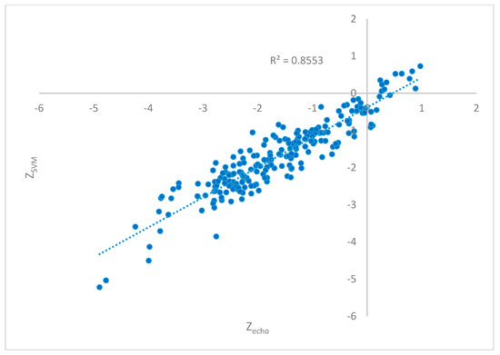
Figure 7.
Scatter diagram of testing data showing SVM predicted depths (m) from Sentinel-2 images (ZSVM) vs. echo sounder depth (Zecho) from field data points for Candás.
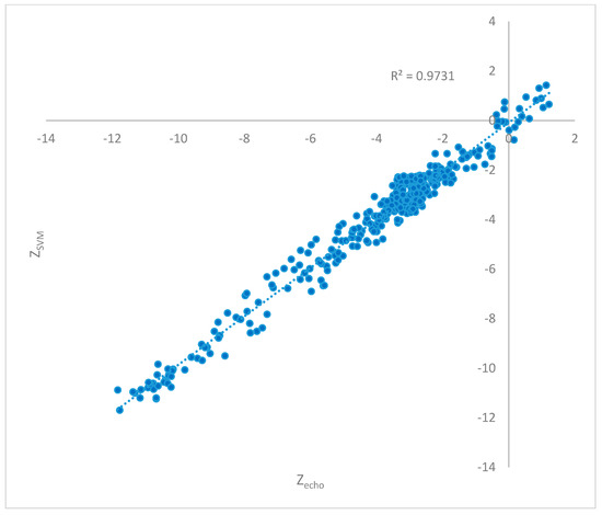
Figure 8.
Scatter diagram of testing data showing SVM predicted depths (m) from Sentinel-2 images (ZSVM) vs. echo sounder depth (Zecho) from field data points for Luarca.
In addition, the relative error of the average depth at the port was calculated using the training and testing dataset (Table 8). The relative error values were 22.05% and 9.04% for Candás and Luarca, respectively. It is greater in Candás because the average depth there is less. In order to obtain a more representative average error for depth, also the error in the average range of depths was calculated. In this case, the errors were 10.76% in Candás and 5.43% in Luarca for the training dataset, and 8.74% in Candás and 4.83% in Luarca for the testing dataset. Despite high relative errors, it is important to note that the objective of the work is that the surface generated by means of the dimensions that were obtained should reflect reality and detect conflictive areas that are in need of dredging. Therefore, although the error is important, it is less so than the general behavior of the generated surface.
Table 8.
Results of the relative error when comparing the SVM predicted and in situ measurement values of depth.
Figure 9 and Figure 10 represent the bathymetry maps of Candás and Luarca that were obtained using the echo sounder in situ measurements and SVM algorithms.
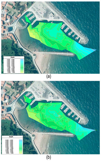
Figure 9.
Bathymetry maps of Candás obtained using (a) echo sounder in situ measurements (Zecho); (b) SVM (ZSVM). The colors denote the depth of the water in meters.
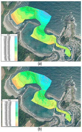
Figure 10.
Bathymetry maps of Luarca obtained using (a) echo sounder in situ measurements (Zecho); (b) SVM (ZSVM). The colors denote the depth of the water in meters.
In the estimated bathymetries that are shown in Figure 9a and Figure 10a, one can detect the transitions and changes in depth in the ports that were studied using this methodology. This is very interesting, because in bathymetry, maps are more helpful in detecting the transitions and average behavior of the bottom than the elevation at a specific point. Figure 9 and Figure 10 show that, although the errors are slightly higher in Luarca (Figure 10a), the general behavior of the seabed has been determined in two ports, both in the deepest areas towards the open sea and in the shallowest and sheltered areas. In addition. Figure 9a and Figure 10a show how the algorithm determined correctly the areas of greatest depth and those of lowest depth with smooth transitions, as well as the contour lines of the coasts. In addition, complex areas of very shallow depth, such as the interior dock of the port of Candás (Figure 9a), are also detected correctly.
To complete the study, a detailed image of the behavior of the contour lines obtained from the bathymetry is generated. In the first phase, shallower areas are compared (Figure 11a,b and Figure 12a,b), and in the second phase, zones of greater water depth are compared (Figure 11c,d and Figure 12c,d).
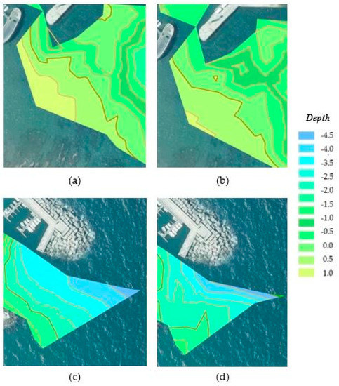
Figure 11.
Details of zoomed areas in bathymetry maps in Candás. (a,c) from echo sounder in situ measurements; (b,d) of SVM depth estimates. The colors denote the depth of the water in meters.
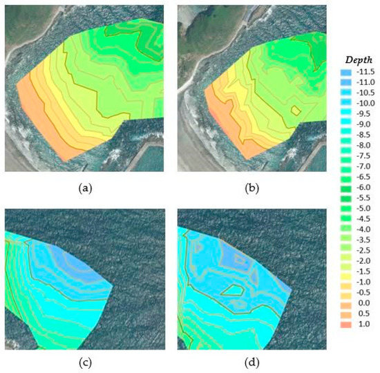
Figure 12.
Details of zoomed areas in the bathymetry maps in Luarca. (a,c) from echo sounder in situ measurements; (b,d) from the SVM depth estimates. The colors denote the depth of the water in meters.
Figure 11 shows some details of zoomed areas to compare the bathymetry maps from the echo sounder in situ measurements to the SVM depth estimates for Candás. In Figure 11a,b, it is revealed that the contour lines have substantially similar shapes and also identify a zone of less depth and, therefore, an area that may need dredging. From Figure 11b,d, it is shown that the representation of the curves is also similar, although the result using an echo sounder indicates a smoother surface. Further, a zone of greater depth is detected in the port. As expected, it was located at the entrance.
In the same way, in Figure 12, they were compared to some details of zoomed areas in Luarca from the echo sounder in situ measurements (Figure 12a,c) and from the SVM depth estimates (Figure 12a,c). In Figure 12a,b, it can be seen that the contour lines have shapes that are substantially similar and parallel to the coastline. In the echo sounder bathymetry, the traces are smoother and better adjusted to the type of bottom with a smooth slope. These results, which were predicted by SVM, are considered to be valid, since they detect correctly the shallowest areas. Finally, in comparing Figure 12c,d, it is seen that the representation of the echo sounder is also smoother. Although the contour lines of the model do not conform precisely to reality, the areas of greater depth are detected.
4. Conclusions
This work was an examination of a technique of remote sensing bathymetry that is based on support vector machine techniques and Sentinel-2 imagery. It was used to estimate the depth in the turbid water of two different ports in the cities of Luarca and Candás in the Principality of Asturias, Spain. The satellite-estimated depth provides an alternative method with which to respond to the increasing demand for coastal topography and bathymetry information in shallow water areas [52]. This approach brings a new perspective to remotely sensed estimated bathymetry. It also provides a high level of accuracy and a cost-effective and efficient solution to the turbid areas of ports, which must be dredged periodically to maintain the free draft and for adequate port management. The visual and statistical results of the study of the ports of Luarca and Candás demonstrate the capacities of the SVM techniques for the prediction of depths from satellite images. The proposed method achieved a greater accuracy for the training dataset in Candás with a mean absolute error of 0.228 m, a root mean squared error of 0.369 m and a coefficient of determination or R2 value of 0.911. The overall errors that were experienced using the testing dataset were a mean absolute error of 0.368 m, a root mean squared error of 0.463 m and a R2 value of 0.855. In the case of Luarca, the SVM method produces depth estimates for the training dataset with a mean absolute error of 0.3274 m, a root mean squared error of 0.441 m and an R2 value of 0.976. The errors in using the testing dataset were a mean absolute error of 0.378 m, a root mean squared error of 0.464 m and an R2 value of 0.973. The low error values obtained in training and testing for both study ports highlight the precision of the bathymetries that were obtained. However, these values are higher than those that other authors obtained [9,23,43,53]. This may be due to the color and turbidity, since the bottoms, which were contaminated and had a muddy composition, have higher light absorption than the sandy bottoms with clear waters that have been analyzed in most studies. Another factor that may have affected these results was the use of a free satellite that has a lower resolution than the satellites that other authors employed. In the future, different artificial neural network techniques should be studied for the estimation of depths with high accuracy from open Sentinel-2 images.
Author Contributions
Conceptualization, V.M.-P. and F.O.-F.; software and validation, V.M.-P. and F.O.-F.; formal analysis, M.C.-B.; data curation, V.M.-P.; writing—original draft preparation, M.C.-B. and V.M.-P.; writing—review and editing, V.M.-P., M.C.-B., and E.P.V.-G.; supervision, F.O.-F. All authors have read and agreed to the published version of the manuscript.
Funding
This work was funded by the Science, Technology and Innovation Plan of the Principality of Asturias (Spain) Ref: FC-GRUPIN-IDI/2018/000225, which is part-funded by the European Regional Development Fund (ERDF).
Acknowledgments
The authors wish to thank to the Port Service and Transport Infrastructures of the Principality of Asturias for the bathymetries from the in situ data collected.
Conflicts of Interest
The authors declare no conflict of interest.
References
- Strayer, D.L.; Malcom, H.M.; Bell, R.E.; Carbotte, S.M.; Nitsche, F.O. Using geophysical information to define benthic habitats in a large river. Freshw. Biol. 2006, 51, 25–38. [Google Scholar] [CrossRef]
- Brown, C.J.; Blondel, P. Developments in the application of multibeam sonar backscatter for seafloor habitat mapping. Appl. Acoust. 2009, 70, 1242–1247. [Google Scholar] [CrossRef]
- Ferretti, R.; Fumagalli, E.; Caccia, M.; Bruzzone, G. Seabed classification using a single beam echosounder. In Proceedings of the OCEANS 2015—Genova, Genoa, Italy, 18–21 May 2015. [Google Scholar]
- O’Hara Murray, R.B.; Gallego, A.G. Data review and the development of realistic tidal andwave energy scenarios for numerical modelling of Orkney Islands waters, Scotland. Ocean Coast. Manag. 2017, 147, 6–20. [Google Scholar] [CrossRef]
- KhaledSeif, A.; Kuroiwa, M.; Abualtayef, M.; Mase, H.; Matsubara, Y. A hydrodynamic model of nearshore waves and wave-induced currents. Int. J. Nav. Archit. Ocean. Eng. 2011, 3, 216–224. [Google Scholar] [CrossRef][Green Version]
- Clementi, E.; Oddo, P.; Drudi, M.; Pinardi, N.; Korres, G.; Grandi, A. Coupling hydrodynamic and wave models: First step and sensitivity experiments in the Mediterranean Sea. Ocean Dynam. 2017, 67, 1293–1312. [Google Scholar] [CrossRef]
- Tang, K.; Pradhan, B. Converting digital number into bathymetric depth: A case study over coastal and shallow Water of Langkawi Island, Malaysia. In Proceedings of the FIG Working Week, Athens, Greece, 24 January 2015. [Google Scholar]
- Mason, D.C.; Gurney, C.; Kennett, M. Beach Topography Mapping—A Comparison of Techniques. J. Coast. Conserv. 2000, 6, 113–124. [Google Scholar] [CrossRef]
- Janowski, L.; Trzcinska, K.; Tegowski, J.; Kruss, A.; Rucinska-Zjadacz, M.; Pocwiardowski, P. Nearshore Benthic Habitat Mapping Based on Multi-Frequency, Multibeam Echosounder Data Using a Combined Object-Based Approach: A Case Study from the Rowy Site in the Southern Baltic Sea. Remote Sens. 2018, 10, 1983. [Google Scholar] [CrossRef]
- Madricardo, F.; Foglini, F.; Kruss, A.; Ferrarin, C.; Pizzeghello, N.M.; Murri, C.; Rossi, M.; Bajo, M.; Bellafiore, D.; Campiani, E.; et al. High Resolution Multibeam and Hydrodynamic Datasets of Tidal Channels and Inlets of the Venice Lagoon. Sci. Data 2017, 4, 170121. [Google Scholar] [CrossRef]
- Horritt, M.S.; Bates, P.D.; Mattinson, M.J. Efects of mesh resolution and topographic representation in 2D finite volume models of shallow water fluvial flow. J. Hydrol. 2006, 329, 306–314. [Google Scholar] [CrossRef]
- Coggins, L.X.; Ghadouani, A. High-resolution bathymetry mapping of water bodies: Development and implementation. Front. Earth Sci. 2019, 7, 330. [Google Scholar] [CrossRef]
- Lyzenga, D.R.; Malinas, N.P.; Tanis, F.J. Multispectral bathymetry using a simple physically based algorithm. IEEE Trans. Geosci. Remote Sens. 2006, 44, 2251–2259. [Google Scholar] [CrossRef]
- Gao, J. Bathymetric mapping by means of remote sensing: Methods, accuracy and limitations. Prog. Phys. Geogr. 2009, 33, 103–116. [Google Scholar] [CrossRef]
- Jégat, V.; Pe’eri, S.; Freire, R.; Klemm, A.; Nyberg, J. Satellite-derived bathymetry: Performance and production. In Proceedings of the Canadian Hydrographic Conference, Halifax, NS, Cannada, 16–19 May 2016. [Google Scholar]
- Hodúl, M.; Bird, S.; Knudby, A.; Chénier, R. Satellite derived photogrammetric bathymetry. ISPRS J. Photogramm. Remote Sens. 2018, 142, 268–277. [Google Scholar] [CrossRef]
- Lyzenga, D. Passive remote sensing techniques for mapping water depth and bottom features. Appl. Opt. 1978, 17, 379–383. [Google Scholar] [CrossRef]
- Lyzenga, D. Remote sensing of bottom reflectance and ater attenuation parameters in shallow water using aircraft and Landsat data. Int. J. Remote Sens. 1981, 2, 71–82. [Google Scholar] [CrossRef]
- Van Hengel, W.; Spitzer, D. Multi-temporal water depth mapping by means of Lansat TM. Int. J. Remote Sens. 1991, 12, 703–712. [Google Scholar] [CrossRef]
- Mishra, D.; Narumalani, S.; Lawson, M.; Rundquist, D. Bathymetric mapping using IKONOS multispectral data. GISci. Remote Sens. 2004, 41, 301–321. [Google Scholar]
- Su, H.; Liu, H.; Heyman, W. Automatic derivation for bathymetric information for multispectral satellite imagery using a non-linear inversion model. Mar. Geod. 2008, 31, 281–298. [Google Scholar] [CrossRef]
- Lyons, M.; Phinn, S.; Roelfsema, C. Inegrating Quickbird multi-spectral satellite and field data: Mapping bathymetry, Seagrass Cover, Seagrass species and change in Moreton bay, Australia in 2004–2007. Remote Sens. 2011, 3, 42–64. [Google Scholar] [CrossRef]
- Misra, A.; Vojinovic, Z.; Ramakrishnan, B.; Luijendijk, A.; Ranasinghe, R. Shallow water bathymetry mapping using Support Vector Machine (SVM) technique and multispectral imagery. Int. J. Remote Sens. 2018, 39, 4431–4450. [Google Scholar] [CrossRef]
- Caballero, I. Assessment of a multi-scene approach with sentinel-2A/B imagery to estimate satellite-derived Bathymetry over moderately turbid regions. In Proceedings of the Poster Presented at the Living Planet Symposium, Milan, Italy, 13–17 May 2019. [Google Scholar]
- Traganos, D.; Poursanidis, D.; Aggarwal, B.; Chrysoulakis, N.; Einartz, P. Estimating satellite-derived bathymetry (SDB) with the google earth engine and sentinel-2. Remote Sens. 2018, 10, 859. [Google Scholar] [CrossRef]
- Drusch, M.; Del Bello, U.; Carlier, S.; Colin, O.; Fernandez, V.; Gascon, F.; Hoersch, B.; Isola, C.; Laberinti, P.; Martimort, P. Sentinel-2: ESA’s Optical High-Resolution Mission for GMES Operational Services. Remote Sens. Environ. 2012, 120, 25–36. [Google Scholar] [CrossRef]
- Caballero, I.; Stumpf, R.P.; Meredith, A. Preliminary assessment of turbidity and chlorophyll impact on bathymetry derived from sentinel-2a and sentinel-3a satellites in south florida. Remote Sens. 2019, 11, 645. [Google Scholar] [CrossRef]
- Almar, R.; Kestenare, E.; Reyns, J.; Jouanno, J.; Anthony, E.; Laibi, R.; Hemer, M.; Du, Y.; Ranasinghe, R. Response of the Bight of Benin (Gulf of Guinea, West Africa) coastline to anthropogenic and natural forcing, part1: Wave climate variability and impacts on the longshore sediment transport. Cont. Shelf Res. 2015, 110, 48–59. [Google Scholar] [CrossRef]
- Bergsma, E.W.; Almar, R.; de Almeida, L.P.M.; Sall, M. On the operational use of uavs for video-derived bathymetry. Coast. Eng. 2019, 152, 103527. [Google Scholar] [CrossRef]
- Liu, S.; Gao, Y.; Zheng, W.; Xiaolu, L. Performance of Two Neural Network Models in Bathymetry. Remote Sens. Lett. 2015, 6, 321–330. [Google Scholar] [CrossRef]
- Wang, Y.; Zhang, P.; Dong, W.; Zhang, Y. Study on Remote Sensing of Water Depths Based on BP Artificial Neural Network. Mar. Sci. Bull. 2007, 9, 26–35. [Google Scholar]
- Ceyhun, Ö.; Yalçın, A. Remote sensing of water depths in shallow waters via artificial neural networks. Estuar. Coast. Shelf. Sci. 2010, 89, 89–96. [Google Scholar] [CrossRef]
- El-Mewafi, M.; Salah, M.; Fawzi, B. Assessment of Optical Satellite Images for Bathymetry Estimation in Shallow Areas Using Artificial Neural Network Model. Am. J. Geogr. Inf. Syst. 2018, 7, 99–106. [Google Scholar]
- Wang, L.; Liu, H.; Su, H.; Wang, J. Bathymetry retrieval from optical images with spatially distributed support vector machines. GISci. Remote Sens. 2019, 56, 323–337. [Google Scholar] [CrossRef]
- Muzirafuti, E.-A.; Barreca, G.; Crupi, A.; Faina, G.; Paltrinieri, D.; Lanza, S.; Randazzo, G. The Contribution of Multispectral Satellite Image to Shallow Water Bathymetry Mapping on the Coast of Misano Adriatico, Italy. J. Mar. Sci. Eng. 2016, 8, 126. [Google Scholar] [CrossRef]
- European Space Agency. European Space Agency, 2019b. ESA Sentinel 2 Orbit Description. Available online: https://sentinel.esa.int/web/sentinel/missions/sentinel-2/satellite-description/orbit (accessed on 29 September 2019).
- European Space Agency. Sentinel-2 MSI Technical Guide. Available online: https://earth.esa.int/web/sentinel/technical-guides/sentinel-2-msi (accessed on 10 September 2019).
- Nowakowski, T. Arianespace Successfully Launches Europe’s Sentinel-2A Earth Observation Satellite; Spaceflight insider: Kourou, French Guiana, 2015. [Google Scholar]
- Kaplan, G.; Avdan, U. Object-based water body extraction model using Sentinel-2 satellite imagery. Eur. J. Remote Sens. 2017, 50, 137–143. [Google Scholar] [CrossRef]
- Poursanidis, D.; Traganos, D.; Reinartz, P.; Chrysoulakis, N. On the use of Sentinel-2 for coastal habitat mapping and satellite-derived bathymetry estimation using downscaled coastal aerosol band. Int. J. Appl. Earth Obs. 2019, 80, 58–70. [Google Scholar] [CrossRef]
- Lanaras, C.; Bioucas-Dias, J.; Galliani, S.; Baltsavias, E.; Schindler, K. Super-resolution of Sentinel-2 images: Learning a globally applicable deep neural network. ISPRS J. Photogramm. 2018, 146, 305–319. [Google Scholar] [CrossRef]
- ESA SNAP. Available online: https://step.esa.int/main/toolboxes/snap (accessed on 12 October 2019).
- Stumpf, R.P.; Holderied, K.; Sinclair, M. Determination of Water Depth with High- Resolution Satellite Imagery over Variable Bottom Types. Limnol. Oceanogr. 2003, 48, 547–556. [Google Scholar] [CrossRef]
- Vapnik, V.; Golowich, S.E.; Smola, A. Support vector method for function approximation, regression estimation, and signal processing. In Advances in Neural Information Processing Systems; MIT Press: Cambridge, MA, USA, 1997; pp. 281–287. [Google Scholar]
- Clarke, S.M.; Griebsch, J.H.; Simpson, T.W. Analysis of support vector regression for approximation of complex engineering analyses. J. Mech. Des. Trans. ASME 2005, 12, 1077–1087. [Google Scholar] [CrossRef]
- Bishop, C.M. Pattern Recognition and Machine Learning; Springer: Berlin, Germany, 2006. [Google Scholar]
- Kranjčić, N.; Medak, D.; Župan, R.; Rezo, M. Support Vector Machine Accuracy Assessment for Extracting Green Urban Areas in Towns. Remote Sens. 2019, 11, 655. [Google Scholar]
- Kuhn, M. Classification and regression training. In R Package Version 6.0–24; 2014; Available online: https://ui.adsabs.harvard.edu/abs/2015ascl.soft05003K/abstract (accessed on 26 June 2020).
- Parameswaran, S.; Weinberger, K.Q. Large margin multi-task metric learning. In Advances in Neural Information Processing Systems; Curran Associates Inc.57: Red Hook, NY, USA, 2010; pp. 1867–1875. [Google Scholar]
- Verrelst, J.; Muñoz, J.; Alonso, L.; Delegido, J.; Rivera, J.P.; Camps-Valls, G.; Moreno, J. Machine learning regression algorithms for biophysical parameter retrieval: Opportunities for Sentinel-2 and -3. Remote Sens. Environ. 2012, 118, 127–139. [Google Scholar] [CrossRef]
- Cowan, G. Statistical Data Analysis; Oxford University Press: Oxford, UK, 1998. [Google Scholar]
- Benveniste, J.; Cazenave, A.; Vignudelli, S.; Fenoglio-Marc, L.; Shah, R.; Almar, R.; Andersen, O.; Birol, F.; Bonnefond, P.; Bouffard, J.; et al. Requirements for a Coastal Hazards Observing System. Front. Mar. Sci. 2019, 6, 348. [Google Scholar] [CrossRef]
- Geyman, E.C.; Maloof, A.C. A simple method for extracting water depth from multispectral satellite imagery in regions of variable bottom type. Earth Space Sci. 2019, 6, 527–537. [Google Scholar] [CrossRef]


© 2020 by the authors. Licensee MDPI, Basel, Switzerland. This article is an open access article distributed under the terms and conditions of the Creative Commons Attribution (CC BY) license (http://creativecommons.org/licenses/by/4.0/).