Evaluating the Preconditions of Two Remote Sensing SWE Retrieval Algorithms over the US

Abstract

A large amount of fresh water resources are stored in the snowpack, which is the primary source of water for streamflow in many places at middle-to-high latitude areas. Therefore, snow water equivalent (SWE) is a key parameter in the water cycle. Active and passive microwave remote sensing methods have been used to retrieve SWE due to relatively poor resolution of current in situ interpolated maps with good accuracy. However, estimation of SWE has proved challenging, despite several decades of efforts to develop retrieval approaches. Active sensors provide higher-resolution observations. Two recent promising retrieval algorithms using active data are dual frequency dual polarization backscattered power and differential interferometry. These retrieval algorithms have some restrictions on snow characteristics, the environment, and instrument properties. The restrictions limit the snow that is suitable for the specific retrieval algorithm. In order to better understand how much of the snowpack satisfies the precondition of these retrieval approaches, we use a 4 km gridded snowpack product over the contiguous US for years 1997 and 2015. We use a simple scattering model to simulate the scattering characteristics of snow. The snow property maps, simulated scattering characteristics of snow, and environmental conditions are used to filter the suitable snow for each retrieval algorithm. We show that snow wetness and vegetation coverage are the two main limiting conditions for these retrieval algorithms. We show that 39% and 44% of the grid-points with snow satisfy the preconditions of dual polarization dual frequency retrieval algorithms at 13.5 GHz (one of the recommended frequencies for this algorithm in the literature) in 1997 and 2015, respectively. The most important limiting factors for dual polarization dual frequency retrieval method are dryness of snow, penetration depth, and vegetation-free constraints. The backscattered power in dual polarization dual frequency method is more sensitive to snow density and grain radius rather than to snow depth. We also show that 55% and 53% of the grid-points with snow satisfy the precondition of differential interferometry retrieval algorithms at 1 GHz (one of the recommended frequencies for this algorithm in the literature) in 1997 and 2015, respectively. The most important precondition-limiting factors for differential interferometry are dryness of snow and vegetation-free constraints. The differential interferometry phase retrieval algorithm is equally sensitive to snow height and snow density variations and is independent of snow grain radius.

1. Introduction

Snow water equivalent (SWE) is a key parameter in the Earth’s energy budget and water cycle. The SWE remains difficult to estimate on a global scale with accuracy and high resolution. Global and daily products relied on passive microwave sensors for the past couple of decades. Data from passive instruments such as the Multichannel Microwave Radiometer (SMMR) and the Special Sensor Microwave Imager (SSM/I) have been used to generate regional and global snow depth and SWE [1]. The Advanced Microwave Scanning Radiometer–EOS instrument (AMSR-E) data have been used in automated algorithms for generating global SWE, at a pixel resolution of 25 km [2]. However, the poor resolution of these datasets and sensitivity to varying snow properties make SWE retrievals challenging over heterogeneous landscapes [3,4].

Airborne LIDAR has been successful in estimating snow height [5]. However, airborne LIDAR is limited to non-cloudy days and regional scale observations. On the other hand, we need a snow density model to estimate SWE using LIDAR snow height.

Active microwave sensors provide high resolution and global coverage. It has been demonstrated that SWE can be retrieved using active microwave remote sensing from space [6,7,8,9,10,11]. Backscattered power from active sensors is used to estimate SWE [6,12,13,14]. QuickSCAT obtained a decade of Ku-band backscatter power. A correlation of 0.97 with a change of 108 mm per dB was observed between QuickSCAT backscattered power and SWE for SWE less than 200 mm [14]. A dual-band (X and Ku) SAR mission called CoReH2O (Cold Regions Hydrology High-resolution Observatory) was proposed as a candidate for the 7th Earth Explorer mission of the European Space Agency (ESA), with the objective to provide SWE products at a spatial resolution of 200 m [12]. However, the mission was not selected to go forward. Cui et al. used bi-continuous vector radiative transfer (bi-continuous-VRT) model as a forward scattering model for SWE estimation [6]. They used X and Ku band dual polarization backscattered power to estimate snow optical thickness and single scattering albedo. A priori characterization of snow structural parameters is of primary importance in the accuracy of SWE retrieval algorithms using backscattered power [6,10,15]. The most common a priori characterization used for SWE retrieval algorithms using backscattered power is grain radius. This has been done using passive data. However, the methods are restricted to passive retrieval errors and also mismatch between active and passive resolutions.

Lightweight and portable frequency modulated continuous wave (FMCW) radars have been used by snow scientists and hydrologists to map snow pack properties, such as depth, SWE, and stratigraphy, rapidly over large distances, at high resolution [16]. However, these sensors cannot be used in spaceborne missions for global coverage due to their wide bandwidth.

The phase of specularly reflected signals from the snowpack has been shown to be strongly dependent on SWE for dry snow and on snow depth for wet snow [11,17]. The phase sensitivity to SWE increases at higher frequencies. However, the phase unwrapping and loss of coherence increase at higher frequencies. Unlike the methods using backscattered power, the sensitivity of the phase change to SWE is very large compared to snow grain size, snow density, snow layering, and ground surface scattering [11]. Therefore, the stratigraphy of the snow has little impact on the SWE retrieval using this method.

Differential interferometric phase is used to estimate SWE [18,19,20]. This method also suffers from phase unwrapping problem and loss of coherence at high frequencies. Methods such as using two frequencies or faster sampling are used to overcome these problems [8,20].

Point snow data are used to generate or improve SWE maps by using various forms of interpolation. Broxton et al. (2016) reduced the error in generating these SWE maps substantially by spatial interpolation of these quantities normalized by accumulated snowfall from the current or previous water years [21]. We use Broxton’s dataset to evaluate two methods for SWE retrieval. The data includes 4.2 km US datasets of snow density (10 layers), snow depth, snow liquid water volume, snow SWE (10 layers), snow fall (mm), precipitation (mm) and mean temperature. Section 2 explains this dataset.

In this study, two promising methods using the data from active sensors are evaluated for SWE retrievals. The first method uses two polarization and two frequency backscattered power values at frequencies higher than X-band [6,10]. The second method uses the interferometric phase between two observations at frequencies lower than X-band [8]. Each method has its own limitations. In this study we evaluate where and when these algorithms are applicable over United States. A simple snow scattering model is developed for a layer of snow over ground, as explained in Section 3. Snow density, depth, and snow wetness (calculated from Broxton’s dataset) are used to calculate different scattering properties of snow such as penetration depth, scattering and absorption coefficients, differential interferometric phase, and backscattered power at different frequencies and polarizations. The amount of snow suitable for SWE retrieval and sensitivity of the first and second retrieval method are quantified in Section 4, Section 4.1, Section 5.1, and Section 5.2, respectively. The limitations and advantages of each method will be discussed.

2. Interpolated In Situ SWE Data over US

Point snow data are used to generate or improve gridded estimates of SWE by using various forms of interpolation. It is challenging to estimate the amount of snow on the ground over large areas due to snow’s strong spatial variability. Broxton et al. show that the spatial interpolation of SWE normalized by accumulated snowfall from the current or previous water years improve SWE estimation substantially [21,22]. By adding gridded precipitation and temperature data to the database, they produce daily maps of SWE and snow depth (available at NSIDC, https://nsidc.org/data/nsidc-0719) across United States. We requested the dataset directly from the University of Arizona so we can had other layers of the dataset, including daily snow density, snow depth, SWE, snow fall, snow liquid water, and mean temperature in a year across United States [22]. We summarize different steps in generating these datasets in Appendix A. We use this dataset to evaluate the regions where radar remote sensing methods can be applicable over the US. The resolution of the data is 4.2 km. We calculate snow wetness or liquid water content, $m_v$, using the liquid water in the snow and snow depth. Data from 1997 and 2015 are used in this study to represent years with high and low precipitation, respectively.

Figure 1a,b show SWE on 1 February of 1997 and 2015, respectively. As seen in Figure 1, SWE is higher on 1 February of 1997 compared to 2015.

Most of the retrieval algorithms including the two discussed in this study assume the snow is dry. We assume the snow is dry if $m_v<2\%$. The snow permittivity and loss factor substantially change for $m_v>2\%$ [23]. We use a tighter threshold of $m_v<1\%$ in figures later in Section 4.1. However, even a small fraction of wetness decreases the penetration depth. Therefore, $m_v$ is used in calculating the penetration depth, as explained in Section 3. Using a tighter threshold for $m_v$ might better represent the dry snow condition. However, we believe using $m_v$ in calculating the snow permittivity and penetration depth together with $m_v<2\%$ limitation are good enough for dry snow condition of these retrieval algorithms. Figure 2a,b shows the number of days with dry snow in October 1996 to September 1997 and October 2014 to September 2015, respectively. Figure 2c,d shows the percentage of number of days with dry snow and number of days with snow in 1997 and 2015, respectively. As shown in these figures, the number of days with dry snow and percentage of days with dry snow are higher in the eastern US in 2015 compared to 1997, whereas they are lower in the western US in 2015 compared to 1997.

3. Simple Scattering Model for Dry Snow

We developed a very simple model for this work to evaluate the performance of SWE retrieval methods [9]. The model consists of a layer of snow on top of the ground. We used this model together with interpolated in situ maps from Section 2 to identify the regions in the US for which SWE retrieval algorithms are applicable in a year in Section 4.1 and Section 5.1. We also use the scattering model in this section to find the sensitivity of retrieval algorithms to different parameters in Section 4.2 and Section 5.2.

The measured microwave emission and backscattering signature of snowpacks motivated the advanced theoretical modeling of volume scattering in a low-loss medium [24,25,26]. For dense media, such as snow, the quantitative treatment of volume scatter has been a difficult task. Because there is a relatively large difference between the dielectric permittivities of air and ice, the conventional Born approximation is not sufficiently accurate. Models have been proposed to cope with this situation, using strong fluctuation theory [26], or SFT, and by dense-medium radiative transfer theory, or DMRT. M$\ddot{a}$tzler used the improved Born approximation model to compute volume backscatter from grain-size depth profiles [24]. It is a simplified SFT model where the mean field is assumed to be given by quasi-static dielectric mixing theory. The advantage of this model is its simplicity and its potential applicability to natural media consisting of complex particles, such as snow firn. Following Oveisgharan et al. [9], we use the improved Born approximation model [24] for the volume scattering from snow volume.

The backscattered power can be written as [6,9].

$${\sigma }_{pq}\left(f\right)={\sigma }_{pq}^g\left(f\right)e^{\frac{-2{\tau }_{pq}\left(f\right)}{cos\theta }}+0.75cos\theta {\omega }_{pq}\left(f\right)(1-e^{\frac{-2{\tau }_{pq}\left(f\right)}{cos\theta }})$$

(1)

where ${\sigma }_{pq}^g,{\tau }_{pq},\theta ,{\omega }_{pq}$ are backscattered power from the ground, optical thickness, incidence angle, and single scattering albedo, respectively. $f,p,$ and q are the frequency, received, and transmitted polarization of the electromagnetic signal, respectively. We use Oh’s model for calculating the backscattered power from ground [27]. Optical thickness and single scattering albedo are related to scattering properties of the snow by

$$\begin{array}{ccc}\hfill {\tau }_{pq}\left(f\right)& =& ({\kappa }_{pq}^s\left(f\right)+{\kappa }_{pq}^a\left(f\right))h\hfill \end{array}$$

(2)

$$\begin{array}{ccc}\hfill {\omega }_{pq}\left(f\right)& =& \frac{{\kappa }_{pq}^s\left(f\right)}{{\kappa }_{pq}^s\left(f\right)+{\kappa }_{pq}^s\left(f\right)}\hfill \end{array}$$

(3)

where ${\kappa }_{pq}^s,{\kappa }_{pq}^a,h$ are scattering coefficient, absorption coefficient, and depth of the snow, respectively. Improved Born Approximation model is used for calculating the scattering and absorption coefficients of snow volume [9,24]. Note that in situ snow wetness is used to calculate the snow permittivity and loss factor and subsequently snow scattering and absorption coefficients. The scattering from air–snow interface and interaction between snow volume and snow–ground interface are neglected because they are very small compared to volume scattering from snow and backscattering from the ground.

We generated a database of backscattered power, scattering and absorption coefficients, and interferometric phase at VV and HV polarization for frequencies equal to 1, 13.5, and 17.25 GHz and snow grain radii equal to 0.2, 0.5, and 0.8 mm. We use snow depth, snow density, and snow wetness maps from Section 2. It is assumed that backscattered signal from the ground is a known parameter in Equation (1) [6]. The backscattered power from the ground is measured at the beginning of the snow season when the ground is snow free and frozen. We assume the backscattering from the ground remains the same during the snow season because of the frozen soil moisture.

4. Using Dual Polarization Dual Frequency Backscattered Power to Estimate SWE

Theoretical studies and experiments explored the relationship between snow volume backscattering and the physical parameters of snow. High frequency radar is more applicable for snow monitoring, as higher frequency bands were found to be more sensitive to snow parameters [28]; in particular, the snow backscattering signal at Ku band is more sensitive than that at X and C bands [14]. Ka-band signals penetrate very little into the snow [29] and do not penetrate all the way to the ground. Hence, Ka-band signals are more useful for measuring snow height using single-pass interferometry. Therefore, X and Ku-bands are the more favorable frequencies for monitoring the snow [6,12].

Radar backscattering signals over snow-covered ground at a given incidence angle $\theta$ can be considered to consist of four components: the surface scattering component from the air—snow interface, a volume scattering component from snowpack, the interaction component between snow volume and snow–ground interface, and the direct ground scattering component. Signals from the air—snow surface can be ignored because for dry snow, these are very small compared with other scattering components at off-nadir incidence angles.

Cui et al. used the bi-continuous vector radiative transfer (bi-continuous-VRT) model, which first constructs snow microstructure similar to real snow and then simulates the snow backscattering signal as a forward model for SWE estimation [6]. They used the model to calculate backscattered power for different snow optical thickness, ${\tau }_{pq,f_i}$, and single scattering albedo, ${\omega }_{pq,f_i}$, where pq refers to VV and VH polarizations and $f_i$ refers to X and Ku-bands. The retrieval algorithm finds the (${\tau }_{VV,X},{\omega }_{VV,X},{\tau }_{HV,X},{\omega }_{HV,X}$) that minimizes the difference between the modeled and measured backscattered power at X and Ku-bands. There are eight unknowns in their algorithm, (${\tau }_{VV,X},{\omega }_{VV,X}$), (${\tau }_{HV,X},{\omega }_{HV,X}$), (${\tau }_{VV,Ku},{\omega }_{VV,Ku}$), and (${\tau }_{HV,Ku},{\omega }_{HV,Ku}$), and four backscattered powers at X and Ku-band at VV and HV polarizations. Using their forward scattering model, they showed a relationship between snow optical thickness and single scattering albedo at X and Ku bands. Therefore, only four unknowns (${\tau }_{VV,X},{\omega }_{VV,X},{\tau }_{HV,X},{\omega }_{HV,X}$) remain.

However, this method assumes the snow is dry and the ground is flat and clear of vegetation. Theoretically, we can model the backscattered power of snow over the slope and under canopies. However, the vegetation cover decreases the sensitivity of backscattered power to SWE [30]. The slope of the ground is considered in the specular component of the backscattered power [10]. However, more studies are needed to evaluate the effect of slope on SWE retrieval accuracy. Cui et al. (2016) applied their SWE retrieval algorithm to the snow over the flat ground [6].

We will use the in situ data from Section 2 to evaluate where and when in the US, the dual polarization dual frequency (hereafter referred to as dual-pol. dual-freq.) retrieval method is applicable. As mentioned earlier in this section, the electromagnetic waves need to penetrate all the way to the ground to capture the SWE of the entire snow depth. Therefore, we present a simple model in Section 3 to calculate the penetration depth of snow using the in situ data in Section 2. Another restriction of this method is that the restricted cost function needs a priori information about the grain radius of the snow [6,10]. We have not included this restriction in evaluating snow, satisfying SWE retrieval limitation in Section 4.1. Many of the SWE retrieval methods using backscattered power use grain radius as an a priori information. Therefore, we evaluate the sensitivity of our simple retrieval algorithm to a priori information about grain radius in Section 4.2.

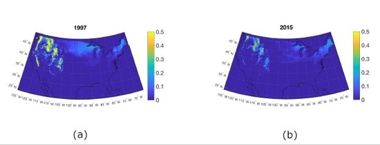
4.1. Snow in the US with Satisfying SWE Retrieval Limitations

In this section, we evaluate what fraction of the snow in one year in the US can be used in a SWE retrieval algorithm using the dual-pol. dual-freq. retrieval algorithm. As mentioned in Section 4, there are some limitations for SWE retrieval algorithm using dual-pol. dual-freq. algorithm. The snow should be dry, the ground should be flat, and the electromagnetic wave should penetrate all the way to the ground. The ground should also be clear of vegetation. We add this as an extra criteria because there has been recent advances in scattering models for snow under vegetation [30].

We use the 4 km gridded SWE and associated snowpack liquid water content map, $m_v$, in Section 2 to identify the regions with dry snow in one year. We assume snow with $m_v<2\%$ is dry in our calculations. The scattering characteristics, including absorption and scattering coefficients, change significantly for $m_v>2\%$ [23], and the same retrieval algorithm is not applicable anymore. However, we also calculate the penetration depth using the liquid water content map.

We use SRTM DEM to find the slope for each location. Figure 3a shows the slope of the ground in the US. Any location with ground slope of less than 5 degrees is considered flat. We use the bare surface fraction estimates using Moderate-Resolution Imaging Spectroradiometer (MODIS) data. The Vegetation Continuous Fields (VCF) collection contains proportional estimates for vegetative cover types: woody vegetation, herbaceous vegetation, and bare ground [23]. The product is derived from all seven bands of the MODIS sensor onboard NASA’s Terra satellite. This VCF product shows how much of a land cover, such as ”forest” or “grassland” exists anywhere on a land surface. The resolution of the data is 210 m × 210 m; therefore, 20 pixels are averaged to match the 4.2 km × 4.2 km resolution of interpolated in situ data. Figure 3b shows the bare surface fraction percentage over the US. Vegetation coverage reduces the sensitivity of SWE retrievals, as expected. There have been recent studies to model scattering from snow under canopies and evaluate the sensitivity of backscattered power to SWE under vegetation [30]. Montomoli et al. (2016) showed by simulated data at Ku-band that the retrieval of SWE is possible in sparse forest if the bare surface fraction remains higher than 70% [30]. They showed that the sensitivity to SWE was too weak for denser forests. In this study, any location in the US with bare surface fraction of less than $1\%$ is considered completely covered with vegetation. Bare surface fraction of $1\%$ for 4.2 km × 4.2 km grid cells is equivalent to 420 × 420 m of the bare ground. We assume that the resolution of active remote sensing (after taking looks for reducing the speckle noise) is much better than 420 m. Therefore, SWE retrieval algorithm can be applied to that 420 × 420 m bare surface ground resolution cell. We can extrapolate the retrieved SWE to other parts of the 4.2 km grid cell. However, for high resolution SWE retrieval, we need to use much higher bare surface fraction thresholds than 1% [30]. On the other hand, SWE retrieval over low vegetation such as grassland is possible even for lower bare surface fraction. However, the scattering model needs to include scattering from vegetation as well. For the sake of simplicity of scattering model, we do not include vegetation type and height maps in this study.

We apply our scattering model in Section 3 to daily-interpolated, in situ snow density, and snow water equivalent over the US at 1, 13.5, and 17.25 GHz. We assume incidence angle is 30 and grain radius is 0.2, 0.5, or 0.8 mm. The incidence angle for most of SAR missions varies between 20 degrees (ERS-1) to 46 degrees (Sentinel-1). We choose 30 degrees as mid-incidence angles between different missions. The scattering and absorption coefficients are calculated to find the penetration depth, $h_{pen}=\frac{1}{{\kappa }_{pq}^s+{\kappa }_{pq}^a}$. The daily calculated penetration depth is compared with daily-interpolated in situ snow depth. Note that in situ snow wetness maps from Section 2 are used both for dryness threshold limitation and calculating penetration depth.

Any snow data in a year that has a flat ground and dry snow with penetration depth greater than snow depth can be used for retrieval algorithm using dual-pol. dual-freq. data.

Table 1. US data satisfying the precondition of the dual polarization dual frequency (dual-pol. dual-freq.) retrieval method in 1997, ($f_1=1$ GHz, $f_2=13.5$ GHz, $f_3=17.25$ GHz, $r_1=0.2$ mm, $r_2=0.5$ mm, $r_3=0.8$ mm).

	${\mathit{f}}_1$	${\mathit{f}}_1$	${\mathit{f}}_1$	${\mathit{f}}_2$	${\mathit{f}}_2$	${\mathit{f}}_2$	${\mathit{f}}_3$	${\mathit{f}}_3$	${\mathit{f}}_3$
	${\mathit{r}}_{\mathbf{1}}$	${\mathit{r}}_{\mathbf{2}}$	${\mathit{r}}_{\mathbf{3}}$	${\mathit{r}}_{\mathbf{1}}$	${\mathit{r}}_{\mathbf{2}}$	${\mathit{r}}_{\mathbf{3}}$	${\mathit{r}}_{\mathbf{1}}$	${\mathit{r}}_{\mathbf{2}}$	${\mathit{r}}_{\mathbf{3}}$
% points over US	66	66	66	55	55	55	53	53	53
$h_{pen}>h$, $slope<5^{\circ }$, $m_v<2\%$
% points over US	46	46	46	39	39	39	38	38	37
$h_{pen}>h$, $slope<5^{\circ }$, $m_v<2\%$, $f_{bare}>1\%$
% of SWE over US	35	35	35	17	17	17	16	16	16
$h_{pen}>h$, $slope<5^{\circ }$, $m_v<2\%$
% of SWE over US	23	23	23	11	11	11	10	10	10
$h_{pen}>h$, $slope<5^{\circ }$, $m_v<2\%$, $f_{bare}>1\%$

shows the ratio of snow during 2019 that dual-pol. dual-freq. retrieval algorithm can be applied. The second row shows the ratio of number of points in US in 1997 with snow that are flat, had dry snow, and in which the electromagnetic wave penetrates all the way to the ground. The fourth row shows the ratio of all SWE in the US in 1997 with the same criteria. Different columns are for different frequencies ($f_1=1$ GHz, $f_2=13.5$ GHz, $f_3=17.25$ GHz) and different grain radii ($r_1=0.2$ mm, $r_2=0.5$ mm, $r_3=0.8$ mm). Note that in ratio calculations, only the data points with snow depth greater than zero are considered. As seen in this table, changing grain radius has almost no impact. This is due to high absorption coefficient compared to scattering coefficient of snow at these frequencies. Note that we also use 1 GHz data in this table. However, the sensitivity of backscattered power to snow properties including SWE is very small at L-band. Hence, L-band backscattered power is not used in dual-pol. dual-freq. retrieval algorithm [6,10]. We use this frequency to show the relative impact of penetration depth compared to snow wetness and ground slope. At 1 GHz, the penetration depth is larger than snow depth in the entire data over the US. Therefore, any limitation in columns two to four is due to snow wetness and ground slope, not penetration depth. As seen in column 2 of this table, $66\%$ of the points with snow and $35\%$ of the total SWE are flat and have dry snow in 1997. However, as mentioned above, columns two to four are irrelevant due to insensitivity of dual-pol. dual-freq. backscattered power to SWE at lower frequencies. Evaluating the accuracy of SWE estimation is beyond the scope of this work. However, we acknowledge that the 1 GHz data is not suitable for this retrieval algorithm [6,10].

By increasing the frequency, the ratio decreases due to decrease of penetration depth. The fourth row ratios in this table are smaller than those in the second row. This means that there are relatively few grid points with lots of SWEs that do not satisfy the precondition of dual-pol. dual. freq. retrieval algorithm. These grid points either have wet snow or large slopes. We know that mountainous areas are not flat and get most of the SWE [31]. Hence, many of these grid cells lie over the mountains. Therefore, we need to enhance the retrieval algorithm for non-flat areas to capture most of the SWEs. As seen in Table 1, more than $50\%$ of spots with snow in the US are not mountainous and can be used in the retrieval algorithm using dual-pol. dual-freq.

The third and fifth columns in Table 1 are similar to second and fourth rows, respectively, with one additional constraint. In third and fifth rows, the bare surface fraction should be more than $1\%$. We assume with a bare surface fraction larger than $1\%$, the electromagnetic waves can directly image the snow with no obstruction from vegetation for at least one radar resolution cell. Adding this constraint affects the results substantially, as expected. Increasing the bare surface fraction threshold to $5\%$ will decrease the the percentage results dramatically. Therefore, there is a need for retrieval models over vegetated areas.

Figure 4 shows the spatial distribution of snow in the US that can be used for retrieval algorithm using dual-pol. dual-freq. Figure 4a shows the percentage of snow in each location in 1997 at 13.5 GHz that is dry, lies on flat ground, and has the electromagnetic wave penetrate all the way to the ground. As shown in this figure, the southern part of the US has a large percentage. Even though these regions get little snow, the snow is generally dry, the ground is flat, and the snow depth is small enough for the waves to penetrate. Figure 4b shows the percentage of snow in each location in 1997 at 13.5 GHz that is dry, lies on flat ground, and allows the electromagnetic wave to penetrate all the way to the ground, and bare surface fraction is greater than $1\%$. As shown in this figure, most of the snow in the eastern US cannot be used with dual-pol. dual-freq retrieval algorithms if there is no SWE retrieval model with good accuracy for snow under vegetation.

Table 2. US data satisfying the precondition of the dual-pol. dual-freq. retrieval method in 2015, ($f_1=1$ GHz, $f_2=13.5$ GHz, $f_3=17.25$ GHz, $r_1=0.2$ mm, $r_2=0.5$ mm, $r_3=0.8$ mm.

	${\mathit{f}}_1$	${\mathit{f}}_1$	${\mathit{f}}_1$	${\mathit{f}}_2$	${\mathit{f}}_2$	${\mathit{f}}_2$	${\mathit{f}}_3$	${\mathit{f}}_3$	${\mathit{f}}_3$
	${\mathit{r}}_{\mathbf{1}}$	${\mathit{r}}_{\mathbf{2}}$	${\mathit{r}}_{\mathbf{3}}$	${\mathit{r}}_{\mathbf{1}}$	${\mathit{r}}_{\mathbf{2}}$	${\mathit{r}}_{\mathbf{3}}$	${\mathit{r}}_{\mathbf{1}}$	${\mathit{r}}_{\mathbf{2}}$	${\mathit{r}}_{\mathbf{3}}$
% points over US	74	74	74	65	65	65	63	63	63
$h_{pen}>h$, $slope<5^{\circ }$, $m_v<2\%$
% points over US	47	47	47	44	44	44	43	43	43
$h_{pen}>h$, $slope<5^{\circ }$, $m_v<2\%$, $f_{bare}>1\%$
% of SWE over US	41	41	41	20	20	20	18	18	18
$h_{pen}>h$, $slope<5^{\circ }$, $m_v<2\%$
% of SWE over US	16	16	16	10	10	10	10	10	10
$h_{pen}>h$, $slope<5^{\circ }$, $m_v<2\%$, $f_{bare}>1\%$

shows the same variables as Table 1 for 2015. The ratios are larger in 2015 for the second, third, and fourth rows. Although the precipitation and number of days with dry snow are lower in 2015, the percentage of the days with dry snow is higher, as also shown in Figure 2. Therefore, the ratios are higher in 2015.

Figure 5a,c,e shows the time series of points with snow from October 1996 to September 1997 with specific physical and observational characteristics at 1, 13.5, and 17.25 GHz, respectively. The blue curve shows the time series of all the snow in one year. The red curve shows the time series of dry snow (that is, with wetness of less than $1\%$). The yellow line shows the time series of the snow that is dry, lays over flat ground, and has depth greater than the penetration depth, as required by dual-pol. dual-freq. retrieval method. The purple curve will be explained in Section 5.1. As seen in this figure, the red (covered mostly by the purple curve) and yellow curves are close at 1 GHz. As the frequency increases and the penetration depth decreases, the yellow curve and red curve become more separate. The other important point in these plots is that the main factor in losing the points suitable for retrieval algorithm is wetness of snow.

Figure 5b,d,f shows the time series of SWE from October 1996 to September 1997 with specific physical and observational characteristics at 1 GHz, 13.5 GHz, and 17.25 GHz, respectively. The different curves are explained above. Note that at 1 GHz, lots of SWE is not suitable for retrieval. The red curve is under the purple curve. Therefore, many SWEs are wet and not usable for retrieval. The deviation of red curve from blue curve starts around day 100 (15 January) which is early in the snow season. This shows that areas with lots of snow have wet snow very early in the season. The yellow curve in Figure 5b is lower than the red curve. The high penetration depth at 1 GHz is not the limitation factor for yellow curve in this figure. Hence, the loss of applicable SWE for retrieval (yellow curve in Figure 5b) is due to ground slope. Therefore, the two major factors violating the condition of dual-pol. dual-freq. retrieval algorithm in Figure 5b are snow wetness and ground slope. However, the dual-pol. dual-freq. retrieval algorithm is not sensitive enough to snow properties at 1 GHZ. Hence, they cannot be considered actual limitations. Comparing Figure 5a,b, we can see that even though these factors have relatively small impacts on the total number of points with snow, they have a large effect on the total SWE in US. This is probably due to the fact that most of the snow volume is in mountainous areas with slopes [31]. Therefore, relatively few points violate the preconditions of the retrieval algorithm, but the SWE on these grid cells is large. The yellow curve in Figure 5d,e drops lower compared to Figure 5b. This is due to snow depth being greater than penetration depth limitation at these frequencies. Therefore, the wetness, large slope, and small penetration depth are the first, second, and third highest limiting factors for the dual-pol. dual-freq. retrieval algorithm, respectively.

Figure 6 is similar to Figure 5 except the plots are for October 2014 to September 2015, a year with relatively low snow precipitation. The plots in parts (a,c,e) are similar to 1997. However, for the time series of SWE in Figure 6a, the yellow plot is very close to the red plot. This means that most of the wet snow is in mountainous areas. Additionally, as shown in Figure 6b,d,e, there is an abrupt loss of suitable SWE for the red and yellow curves beginning in March (day 157). Looking at the US average air temperature, we realized that there was an abrupt warming on that specific day. Therefore, the snow became wet and unsuitable for retrieval algorithm.

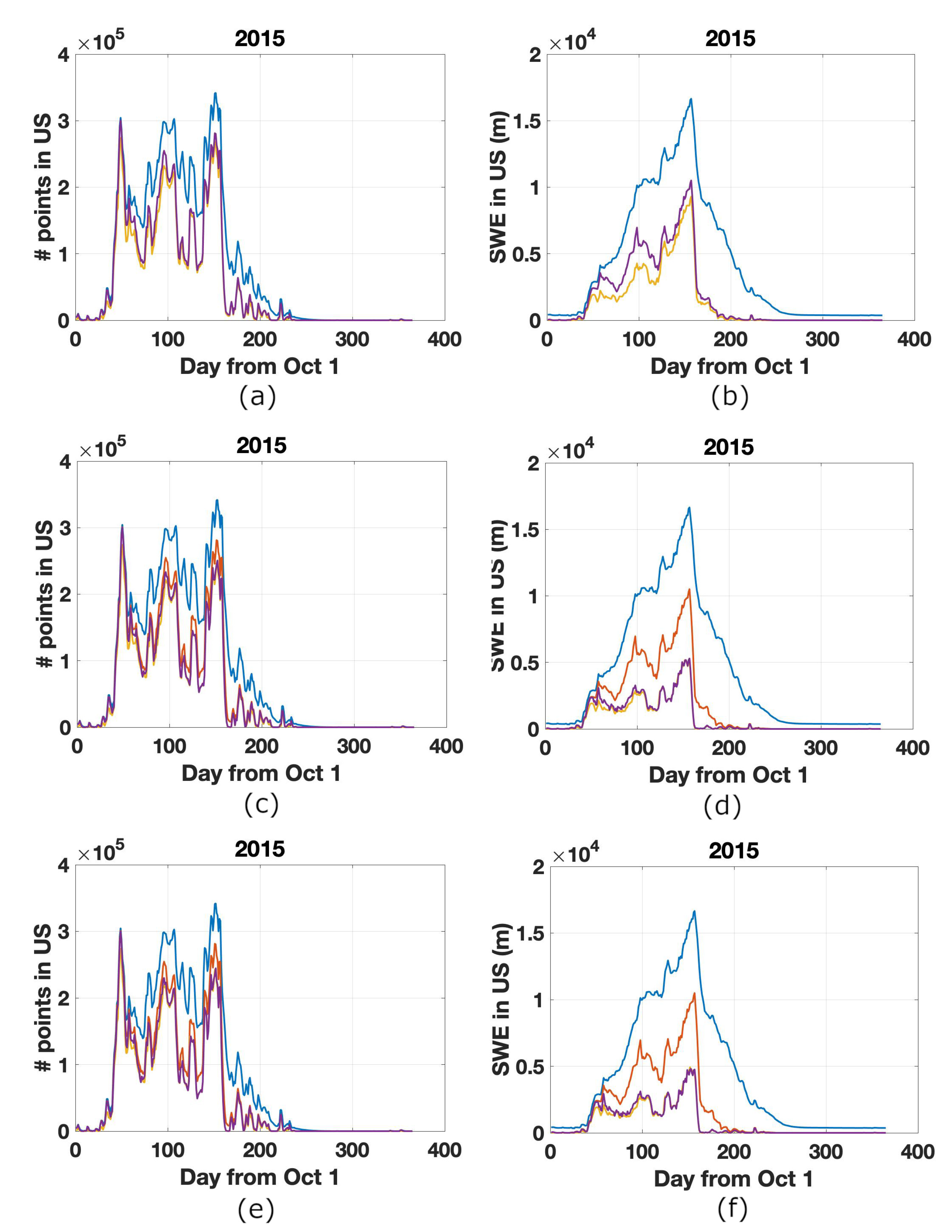
4.2. Sensitivity of Retrieval to Different Parameters

Different parameters have different contributions in the backscattered power. In order to better understand the effects of these parameters on SWE retrieval, we calculate the sensitivity of backscattered power to these parameters. For a simple model described in Section 3, we compute the sensitivity of the backscattered power to grain radius, snow depth, and snow density. In order to calculate the sensitivity of backscattered power to parameter c, we calculate $\frac{\partial \sigma }{\partial c}\times \Delta c$, where $\frac{\partial \sigma }{\partial c}$ is the derivative of backscattered power to parameter c and $\Delta c$ is the variation of parameter c by $20\%$.

Using Equation (1), we can write the sensitivity to grain radius as

$$\frac{\partial \sigma }{\partial r}=\frac{\partial \sigma }{\partial {\kappa }^s}\times \frac{3{\kappa }^s}{r}$$

(4)

where r is the grain radius and

$$\frac{\partial \sigma }{\partial {\kappa }^s}=\frac{2h}{cos\theta }{e}^{\frac{-2\tau }{cos\theta }}(0.75cos\theta \omega -{\sigma }^g)+0.75cos\theta \frac{{\kappa }^a}{{({\kappa }^s+{\kappa }^a)}^2}(1-e^{\frac{-2\tau }{cos\theta }})$$

(5)

Note f and subscripts p and q are not shown in these equations for a simpler presentation.

Figure 7a,b shows the sensitivity of backscattered power to grain radius vs. snow height for snow density equal to 0.15 and 0.45 g/cm${}^3$, respectively. The blue and red curves show the sensitivity to grain radius at 13.5 GHz for grain radii equal to 0.3 and 0.9 mm, respectively. The yellow and purple curves show the sensitivity to grain radius at 17.25 GHz for grain radii equal to 0.3 and 0.9 mm, respectively.

The sensitivity of backscattered power to snow density can be written as

$$\frac{\partial \sigma }{\partial \rho }=\frac{\partial \sigma }{\partial {\kappa }^s}\times \frac{\partial {\kappa }^s}{\partial \rho }+\frac{\partial \sigma }{\partial {\kappa }^a}\times \frac{\partial {\kappa }^a}{\partial \rho }$$

(6)

where

$$\frac{\partial \sigma }{\partial {\kappa }^a}=\frac{2h}{cos\theta }{e}^{\frac{-2\tau }{cos\theta }}(0.75cos\theta \omega -{\sigma }^g)-0.75cos\theta \frac{{\kappa }^s}{{({\kappa }^s+{\kappa }^a)}^2}(1-e^{\frac{-2\tau }{cos\theta }})$$

(7)

Figure 8a,b shows the variation of $\frac{{\kappa }^s}{r^3}$ and ${\kappa }^a$ with respect to snow density, respectively. The orange and green curves show the coefficients for 13.5 and 17.25 GHz, respectively. We can fit a polynomial to both curves with degree of 4 and 2 to $\frac{{\kappa }^s}{r^3}$ and ${\kappa }^a$, respectively. Therefore, we can calculate the $\frac{\partial {\kappa }^s}{\partial \rho }$ and $\frac{\partial {\kappa }^a}{\partial \rho }$ by calculating the derivatives of fitted polynomials at different frequencies. Note that using more sophisticated scattering models such as DMRT show that the extinction coefficient decreases for densities greater than 0.2 g/cm${}^3$ [32] which contradicts the results in Figure 8. We use the improved Born approximation for fast and simple calculation of scattering coefficients. Comparing different scattering models for snow is beyond the scope of this work and will be the future of this study.

Figure 7b,e shows the sensitivity of backscattered power to snow density vs. snow depth for snow density equal to 0.15 and 0.45 g/cm${}^3$, respectively. The blue and red curves show the sensitivity to snow density at 13.5 GHz for grain radii equal to 0.3 and 0.9 mm, respectively. The yellow and purple curves show the sensitivity to snow density at 17.25 GHz for grain radii equal to 0.3 and 0.9 mm, respectively.

The sensitivity of backscattered power to snow depth can be simplified to

$$\frac{\partial \sigma }{\partial h}=\frac{2({\kappa }^s+{\kappa }^a)}{cos\theta }{e}^{\frac{-2\tau }{cos\theta }}(0.75cos\theta \frac{{\kappa }^s}{{\kappa }^a+{\kappa }^s}-{\sigma }^g)$$

(8)

Figure 7c,f shows the sensitivity of backscattered power to snow depth vs. snow depth for snow density equal to 0.15 and 0.45 g/cm${}^3$, respectively. The blue and red curves show the sensitivity to snow depth at 13.5 GHz for grain radii equal to 0.3 and 0.9 mm, respectively. The yellow and purple curves show the sensitivity to snow depth at 17.25 GHz for grain radii equal to 0.3 and 0.9 mm, respectively.

As seen in Figure 7a–c, the sensitivity of backscattered power to grain radius, snow density, and snow depth is linear vs. snow depth for small snow density. However, the sensitivity of backscattered power saturates at larger snow depths for large snow density, as shown in Figure 7d–f. This is due to the fact that the waves do not reach to the ground and backscattered power itself saturates too. As seen in Figure 7, the backscattered power is most sensitive to grain radius and snow density and less sensitive to snow depth. These figures show how the error in a priori information for any of these parameters can affect the retrieved SWE. Note that we use a very simple one layer of snow over ground in this sensitivity analysis. The variation of snow density and grain size through depth is not included, nor is double-bouncing between snow and the ground. Consequently, those things may have affected the sensitivity values in Figure 7a–f. However, the relative effects of different parameters remain valid.

5. Using Differential Interferometry to Estimate SWE

Differential SAR interferometry measures the signal delay relative to the radar wavelength to detect small surface elevation changes over large areas with a vertical accuracy of a few millimeters [33,34]. The effect of volume scattering of dry snow on interferometric phase is very small compared to scattering from the ground. The snow volume scattering affects the interferometric phase for very deep snow at higher frequencies such as C-band [9]. However, the reflected signal is delayed by the snow volume due to its refractive index. The measured phase difference is proportional and very sensitive to small changes in SWE variation ($\Delta SWE$) [18]. However, the loss of coherence between the observations and phase unwrapping are the main limitations for SWE retrieval using differential interferometry. Melting and wind are the main reasons for low temporal coherence [8,35]. A high temporal coherence is observed at L-band for dry snow with a month temporal baseline [36]. Temporal coherence decreases with increasing frequency [8]. A median temporal coherence of about 0.5 is observed at 10.2 GHz and 16.8 GHz even after 60 days [8] for a controlled system. However, the spacebone TerraSAR-X temporal coherence over snow at 9.65 GHz reduces significantly in 11 days [7]. This is probably due to random phase drifts over time that cannot be estimated and corrected in a spaceborne system compared to a ground radar. Vegetation cover decreases the temporal coherence significantly at high frequencies [37]. More studies are needed to better model temporal coherence at different frequencies, different land types, and different environmental condition. Therefore, we do not include temporal coherence as a limitation in this study. With current SnowEx 2020 campaign using Uninhabited Aerial Vehicle Synthetic Aperture Radar (UAVSAR) L-band differential interferometry data and future NASA-ISRO SAR (NISAR) L-band data, there will be more advances in the limitations and capabilities of this method.

Despite these problems, different techniques are used to resolve these problems for successful SWE estimation [38,39]. Leinss et al. used two frequency and fast sampling to reconstruct lost phase cycles from phase-wrapping and avoid loss of coherence.

For dry snow a few meters deep and with frequencies below 20 GHz, the volume scattering effect on interferometric phase is negligible. However, low temporal coherence and low penetration depth at frequencies higher than 10 GHz, make L and C-band desirable frequencies for differential interferometry. The signal delay caused by refraction can be measured with differential radar interferometry as [8]:

$$\Delta \varphi =-2{\kappa }_i(cos\theta -\sqrt{ϵ-{sin}^2\theta })\Delta h$$

(9)

where $\Delta \varphi ,{\kappa }_i,\Delta h,\theta ,$ and $ϵ$ are interferometric phase between two days, incidence wavenumber, snow depth change, incidence angle, and permittivity of the snow, respectively. The change in interferometric phase is used to calculate $\Delta SWE$ [8]. Similar to dual-pol. dual-freq. retrieval algorithm, this technique relies on dryness of snow in order to penetrate all the way to the ground. Therefore, penetration depth of snow should be larger than snow depth. Single-pass interferometry on the other hand, measures the snow height due to small penetration of Ka-band signals into the snow [29]. Therefore, snow can be either dry or wet. Our analysis here are based on differential interferometry retrieval algorithm not single-pass interferometry. Hence, the snow should be dry. We cannot evaluate the temporal coherence at different frequencies using our database. Temporal coherence loss is a very big limitation for this retrieval algorithm. Evaluating temporal coherence needs a rich interferometric dataset at different frequencies and is beyond the scope of this work. However, we can apply the phase variation between two consecutive days to be less than $2\pi$ to avoid the phase unwrapping problem.

5.1. Snow in US with Satisfying SWE Retrieval Limitations

In this section, we evaluate what fraction of the snow in one year in the US can be used in SWE retrieval algorithm using interferometric phase retrieval algorithm. As mentioned in Section 5, there are some limitations for SWE retrieval algorithm using interferometric phase change algorithm. The snow should be dry, the electromagnetic wave should penetrate all the way to the ground, and the phase change between two days should be smaller than $2\pi$. The ground should also be clear of vegetation. We add this as an extra criteria because the retrieval algorithm can be modified for a region with vegetation.

Similar to Section 4.1, we use the 4 km gridded SWE and associated snowpack liquid water content map, $m_v$, in Section 2 to identify the regions with dry snow in one year with $m_v<2\%$ as dryness threshold. We also use the liquid water content and snow density maps to calculate the penetration depth. Differential interferometric phase retrieval algorithm is not applicable to the snow with penetration depth smaller than snow depth i. We calculate the phase change due to snow height variation between any consecutive days. Only the snow with daily interferometric phase change less than $2\pi$ is considered for retrieval algorithm to avoid phase unwrapping problem. However, the revisit time for future SWE measurement missions using interferometric phase is most probably longer than one day. We use one day as an ideal revisit time for a system. However, we show later in this section that other parameters such as vegetation cover and snow dryness are the limiting factors compared to phase change due to snow depth variation. Note that temporal coherence (the major limitation of this retrieval algorithm) is not considered in this study due to lack of available data at this study.

Similar to Section 4.1, we use the bare surface fraction in Figure 3b with a threshold of $1\%$.

We apply our scattering model in Section 3 to daily-interpolated, in situ snow density, snow water equivalent, and snow liquid water content over the US at 1 GHz, 13.5 GHz, and 17.25 GHz. We assume incidence angle is 30 and grain radii are 0.2 mm, 0.5 mm, or 0.8 mm. The scattering and absorption coefficients are calculated to find the penetration depth, $d=\frac{1}{{\kappa }_{pq}^s+{\kappa }_{pq}^a}$. The daily calculated penetration depth is compared with daily-interpolated, in situ snow depth.

For the daily-interpolated, in situ snow density and snow depth variation between two days from Section 2, we calculate the phase change between any two consecutive days. The result should be less than $2\pi$ to avoid the unwrapping problem. Any snow data in a year that has dry snow with penetration depth greater than snow depth and a daily phase change of less than $2\pi$ can be used for retrieval algorithm using interferometric phase change.

Table 3. US data satisfying the preconditions of differential interferometry retrieval method in 1997, ($f_1=1$ GHz, $f_2=13.5$ GHz, $f_3=17.25$ GHz, $r_1=0.2$ mm, $r_2=0.5$ mm, $r_3=0.8$ mm).

	${\mathit{f}}_1$	${\mathit{f}}_1$	${\mathit{f}}_1$	${\mathit{f}}_2$	${\mathit{f}}_2$	${\mathit{f}}_2$	${\mathit{f}}_3$	${\mathit{f}}_3$	${\mathit{f}}_3$
	${\mathit{r}}_{\mathbf{1}}$	${\mathit{r}}_{\mathbf{2}}$	${\mathit{r}}_{\mathbf{3}}$	${\mathit{r}}_{\mathbf{1}}$	${\mathit{r}}_{\mathbf{2}}$	${\mathit{r}}_{\mathbf{3}}$	${\mathit{r}}_{\mathbf{1}}$	${\mathit{r}}_{\mathbf{2}}$	${\mathit{r}}_{\mathbf{3}}$
% points over US	77	77	77	58	58	58	55	55	55
$h_{pen}>h$, $m_v<2\%$, daily $\Delta \varphi <2\pi$
% points over US	55	55	55	41	41	41	39	39	39
$h_{pen}>h$, $m_v<2\%$, daily $\Delta \varphi <2\pi$, $f_{bare}>1\%$
% of SWE over US	72	72	72	19	19	19	17	17	16
$h_{pen}>h$, $m_v<2\%$, daily $\Delta \varphi <2\pi$
% of SWE over US	53	53	53	12	12	12	11	11	11
$h_{pen}>h$, $m_v<2\%$, daily $\Delta \varphi <2\pi$, $f_{bare}>1\%$

shows the ratio of snow during 1997 to which differential interferometry retrieval algorithm can be applied. The second row shows the ratio of number of points in the US in 1997 with snow that has dry snow, no daily phase change ambiguity, and electromagnetic wave penetration depth greater than snow depth. The fourth row shows the ratio of all SWE in US in 1997 with the same criteria. Different columns are for different frequencies ($f_1=1$ GHz, $f_2=13.5$ GHz, $f_3=17.25$ GHz) and different grain radii ($r_1=0.2$ mm, $r_2=0.5$ mm, $r_3=0.8$ mm). Note that in ratio calculation only the data point with snow depth greater than zero are considered. As seen in this table, changing grain radius has almost no impact. This is due to the high absorption coefficient compared to the scattering coefficient of snow at these frequencies. At 1 GHz, the penetration depth is larger than the snow depth in the entire data over US. Therefore, $77\%$ of the points with snow and $72\%$ of the total SWE had dry snow in 1997. By increasing the frequency, the ratio decreases due to decrease of penetration depth.

The third and fifth columns in Table 3 are similar to second and fourth rows, respectively, with one additional constraint. In third and fifth rows, the bare surface fraction should be more than $1\%$. We assume with bare surface fraction larger than $1\%$, the backscattering wave has a direct backscattering component from the snow with no obstruction from vegetation. Therefore, SWE variation affects the differential interferometric phase. Adding this constraint affects the results substantially as expected. Increasing the bare surface fraction threshold to $5\%$ will decrease the the percentage results dramatically. Therefore, there is a need for retrieval models over vegetated areas.

Note that fourth and fifth row ratios are very sensitive to frequency change. The loss in the ratio from 1 GHz to 13.5 GHz is due to the fact that the penetration depth becomes less than the snow depth. Therefore, much of the snow with large snow depth and SWE can not be used for retrieval algorithm. These areas are limited in space but have lots of snow. Hence, the fourth and fifth rows are affected more than second and third.

Table 4. US data satisfying the preconditions of the differential interferometry retrieval method in 2015, ($f_1=1$ GHz, $f_2=13.5$ GHz, $f_3=17.25$ GHz, $r_1=0.2$ mm, $r_2=0.5$ mm, $r_3=0.8$ mm).

	${\mathit{f}}_1$	${\mathit{f}}_1$	${\mathit{f}}_1$	${\mathit{f}}_2$	${\mathit{f}}_2$	${\mathit{f}}_2$	${\mathit{f}}_3$	${\mathit{f}}_3$	${\mathit{f}}_3$
	${\mathit{r}}_{\mathbf{1}}$	${\mathit{r}}_{\mathbf{2}}$	${\mathit{r}}_{\mathbf{3}}$	${\mathit{r}}_{\mathbf{1}}$	${\mathit{r}}_{\mathbf{2}}$	${\mathit{r}}_{\mathbf{3}}$	${\mathit{r}}_{\mathbf{1}}$	${\mathit{r}}_{\mathbf{2}}$	${\mathit{r}}_{\mathbf{3}}$
% points over US	82	82	82	68	68	68	66	66	66
$h_{pen}>h$, $m_v<2\%$, daily $\Delta \varphi <2\pi$
% points over US	53	53	53	47	47	47	46	46	46
$h_{pen}>h$, $m_v<2\%$, daily $\Delta \varphi <2\pi$, $f_{bare}>1\%$
% of SWE over US	60	60	60	21	21	21	20	19	19
$h_{pen}>h$, $m_v<2\%$, daily $\Delta \varphi <2\pi$
% of SWE over US	32	32	32	12	12	12	11	11	11
$h_{pen}>h$, $m_v<2\%$, daily $\Delta \varphi <2\pi$, $f_{bare}>1\%$

is the same as Table 3 but for 2015. The observed pattern is similar to 1997. However, the percentage of points suitable for differential interferometry retrieval method is larger in 2015 compared to 1997. The SWE percentage, on the other hand, is smaller in 2015. Therefore, areas with lots of snow are not suitable for this method in 2015. It shows that the snow in mountainous regions is wetter in 2015 [31].

We calculate the interferometric phase change due to snow depth change after 2, 6, and 12 days and generate a table similar to Table 3. We change the daily $\Delta \varphi <2\pi$ criteria to 2, 6, and 12 days $\Delta \varphi <2\pi$. The performance degrades less than $2\%$ compared to Table 3. Therefore, the snow wetness and bare surface fraction parameter are the limiting factors compared to phase unwrapping. Note that temporal coherence is not considered in this study. Temporal coherence is highly dependent on revisit time and frequency. At C and S-band, the temporal coherence drops substantially even after a day or two [35]. Therefore, at higher frequencies such as X and Ku-band, low temporal coherence limits SWE retrieval algorithm and fast revisit time is required. Therefore, differential interferometry works at lower frequencies such as L-band or higher frequencies with very rapid revisit time.

The purple curves in Figure 5 and Figure 6 show the time series of points and SWE with dry snow (wetness less than $1\%$), penetration depth greater than snow depth, and daily differential phase difference less than $2\pi$, as required by the differential phase interferometry retrieval algorithm. The purple curve in all these plots is slightly higher than yellow curve except Figure 5b. This is similar to the pattern in Table 1, Table 2, Table 3 and Table 4. The penetration depth at 1 GHz exceeds the snow depth, and dryness of the snow is the only limitation for differential phase interferometry. Therefore, the purple curve and red curve lie on top of each other in Figure 5b. However, the flatness requirement decreases the suitable SWE for dual-pol. dual-freq. retrieval algorithm.

5.2. Sensitivity of Retrieval to Different Parameters

As seen in Equation (9), snow permittivity and snow depth are the only two snow parameters that affect the interferometric phase change. Snow permittivity varies with snow density and is independent of observed frequency. In order to better understand the effect of these two parameters on SWE retrieval, we calculate the sensitivity of interferometric phase to snow density and snow depth. For a simple model described in Section 3, we compute the sensitivity of the interferometric phase to snow depth and snow density. Similar to Section 4.2, we use $\Delta c=20\%$.

Using Equation (9), we can write the sensitivity to snow depth as

$$\frac{\partial \Delta \varphi }{\partial \Delta h}=-2{\kappa }_i(cos\theta -\sqrt{ϵ-{sin}^2\theta })$$

(10)

Figure 9a,c shows the sensitivity of interferometric phase change in radians to snow depth in meter vs. snow depth at 1 GHz and 13.5 GHz, respectively. The blue, red, and orange curves show the sensitivity to snow depth for snow density equal to 0.15, 0.3, and 0.45 g/cm${}^3$, respectively. As seen in these two figures, there is a linear relationship between snow sensitivity and snow depth. Additionally, increasing the observation frequency increases the sensitivity as expected. As shown in Figure 9c, the differential phase variation due to a $20\%$ change in snow height at 13.5 GHz easily exceeds $2\pi$ at snow depth greater than 50 cm. At 1 GHz, a $20\%$ variation in snow depth never exceeds $2\pi$ and the phase change remain unambiguous. Therefore, increasing the frequency increases sensitivity to snow height variation; however, phase unwrapping becomes a problem and we need to resolve it by other technique such as different polarization observations.

Using Equation (9), we can write the sensitivity to snow density as

$$\frac{\partial \Delta \varphi }{\partial \rho }={\kappa }_i\Delta h\frac{\frac{\partial ϵ}{\partial \rho }}{\sqrt{ϵ-{sin}^2\theta }}$$

(11)

We need to calculate $\frac{\partial ϵ}{\partial \rho }$ in Equation (11) to calculate $\frac{\partial \Delta \varphi }{\partial \rho }$. Figure 10 shows $ϵ$ vs. snow density. We fit a 2-degree polynomial to this curve and use its derivative to calculate the $\frac{\partial ϵ}{\partial \rho }$. Note that the permittivity is independent of observed frequency.

Figure 9b,d shows the sensitivity of interferometric phase change to snow density vs. snow depth at 1 GHz and 13.5 GHz, respectively. The blue, red, and orange curves show the sensitivity to snow density for snow density equal to 0.15, 0.3, and 0.45 g/cm${}^3$, respectively. The plots are very similar to Figure 9a,c. Therefore, the sensitivity of differential phase variation due to snow height variation and snow density variation is almost the same.

6. Conclusions

In this study we identify the regions and the amount of snow in the US that satisfy the pre-condition of the two major SWE retrieval algorithms. We used the interpolated in situ data to calculate scattering properties of snow. From the scattering properties together with interpolated data, we have snow depth, SWE, snow wetness, and snow penetration depth at different frequencies. We used these parameters, the vegetation fraction map, and the slope of the ground map to evaluate the preconditions of each method.

We used a very simple single layer of snow over ground to calculate scattering properties in this work. The simple model enables us to generate global snow scattering properties for two years easily and quickly. However, this model neglects the double bounce between snow and ground. Additionally, the variation of snow grain radius and snow density through depth is neglected in this model. Other sophisticated scattering models such as bi-continuous-VRT or DMRT can be used to better model the snow scattering properties [6,32,40,41]. The other limiting factor that we did not include in this study is that a very thin layer of snow (between 10–20 mm) is beyond the sensitivity of these algorithms [6,8].

We showed that the dryness condition of snow reduces the percentage of snow to which we can apply the retrieval algorithms significantly. The non-vegetated condition is also a notable restriction in both retrieval algorithms. Therefore, retrieval models need to be improved to be able to retrieve snow under vegetation. The other limiting factor for dual-pol. dual-freq. method is flat ground at lower frequencies, as shown, for instance, in Figure 5b. However, the dual-pol. dual-freq. retrieval method works better at higher frequencies because of its sensitivity to snow properties [6,10]. The small penetration depth at higher frequencies is the limiting factor in areas with deep snow, as shown in Figure 5d. The deep snow mostly lays on mountainous areas, as shown in Figure 1 [31]. Hence, the penetration depth is the limiting factor rather than flat ground restriction at higher frequencies. Therefore, the most important limiting factors for the dual freq. dual pol. retrieval method are dryness of snow, penetration depth, and vegetation-free constraints.

The phase unwrapping restriction for differential interferometric phase retrieval algorithm has a smaller effect than small penetration depth at higher frequencies. However, differential interferometric phase retrieval method works better at lower frequencies because of higher temporal correlation. Therefore, the most important limiting factors for differential interferometry are dryness of snow and vegetation-free constraints.

We show that 39% and 44% of the grid-points with snow satisfy the preconditions of dual pol. dual freq. retrieval algorithms at 13.5 GHz (one of the recommended frequencies for this algorithm [6,10]) in 1997 and 2015, respectively. On the other hand, 55% and 53% of the grid-points with snow satisfy the preconditions of differential interferometry retrieval algorithms at 1 GHz (one of the recommended frequencies for this algorithm [8]) in 1997 and 2015, respectively. However, we used $m_v<2\%$ limitation. Lower wetness threshold may be applied for a tighter precondition and to reduce these numbers. Improving these algorithms to be able to retrieve snow under vegetation with a good accuracy increases the grid-points with snow satisfying the preconditions of these algorithms by at least 16%. Therefore, modifying these algorithm for snow under vegetation is very important.

We also quantified the sensitivity of these two algorithms to different parameters of snow. We showed that the sensitivity of the observations increases as the frequency increases. The dual-pol. dual-freq. retrieval algorithm is most sensitive to grain radius and snow density variation and less sensitive to snow depth variation. Therefore, retrieving snow height is challenging. The backscattered power variation vs. snow depth saturates for high snow density. Therefore, the retrieval algorithm accuracy decreases when snow is denser.

The differential interferometry phase retrieval algorithm is equally sensitive to snow height and snow density variations. The phase variation at higher frequency causes phase unwrapping problem. However, high frequencies are not favorable for this retrieval method.

Therefore, if the accuracy of two methods are similar, the differential interferometry method seems to be applicable to more snow with more sensitivity to snow height. However, the performance of differential interferometry retrieval method degrades significantly with low temporal coherence. On the other hand, the dual-pol dual-freq. retrieval method needs a priori information such as grain radius for non-ambiguous retrieval. For a fair comparison between these two methods, we need to find a way to consider these limitations in our future studies. The accuracies of these methods were not evaluated in this study, and they need investigation.

References

1. Pulliainen, J.; Hallikainen, M. Retrieval of regional snow water equivalent from space-borne passive microwave observations. Remote Sens. Environ. 2001, 75, 76–85. [Google Scholar] [CrossRef]
2. Kelly, R.E.; Chang, A.T.; Tsang, L.; Foster, J.L. A prototype AMSR-E global snow area and snow depth algorithm. IEEE Trans. Geosci. Remote Sens. 2003, 41, 230–242. [Google Scholar] [CrossRef] [Green Version]
3. Takala, M.; Luojus, K.; Pulliainen, J.; Derksen, C.; Lemmetyinen, J.; Kärnä, J.P.; Bojkov, B. Estimating northern hemisphere snow water equivalent for climate research through assimilation of space-borne radiometer data and ground-based measurements. Remote Sens. Environ. 2011, 115, 3517–3529. [Google Scholar] [CrossRef]
4. Kelly, R. The AMSR-E Snow depth algorithm: Description and initial results. J. Remote Sens. Soc. Jpn. 2009, 29, 307–317. [Google Scholar]
5. Painter, T.H.; Berisford, D.F.; Boardman, J.W.; Bormann, K.J.; Deems, J.S.; Gehrke, F.; Hedrick, A.; Joyce, M.; Laidlaw, R.; Marks, D.; et al. The Airborne Snow Observatory: Fusion of scanning LiDAR, imaging spectrometer, and physically-based modeling for mapping snow water equivalent and snow albedo. Remote Sens. Environ. 2016, 184, 139–152. [Google Scholar] [CrossRef] [Green Version]
6. Cui, Y.; Xiong, C.; Lemmetyinen, J.; Shi, J.; Jiang, L.; Peng, B.; Li, H.; Zhao, T.; Ji, D.; Hu, T. Estimating Snow Water Equivalent with Backscattering at X and Ku Band on Absorption Loss. Remote Sens. 2016, 8, 505. [Google Scholar] [CrossRef] [Green Version]
7. Leinss, S.; Parrella, G.; Hajnsek, I. Snow Height Determination by Polarimetric Phase Differences in X-Band SAR Data. IEEE J. Sel. Top. Appl. Earth Obs. Remote Sens. 2014, 7, 3794–3810. [Google Scholar] [CrossRef] [Green Version]
8. Leinss, S.; Wiesmann, A.; Lemmetyinen, J.; Hajnsek, I. Snow Water Equivalent of Dry Snow Measured by Differential Interferometry. IEEE J. Sel. Top. Appl. Earth Obs. Remote Sens. 2015, 8, 3773–3790. [Google Scholar] [CrossRef] [Green Version]
9. Oveisgharan, S.; Zebker, H. Estimating Snow Accumulation From InSAR Correlation Observations. IEEE Trans. Geosci. Remote Sens. 2007, 45, 10–20. [Google Scholar] [CrossRef]
10. Lemmetyinen, J.; Derksen, C.; Rott, H.; Macelloni, G.; King, J.; Schneebeli, M.; Wiesmann, A.; Leppanen, L.; Kontu, A.; Pulliainen, J. Retrieval of Effective Correlation Length and Snow Water Equivalent from Radar and Passive Microwave Measurements. Remote Sens. 2018, 10, 170. [Google Scholar] [CrossRef] [Green Version]
11. Yueh, S.H.; Xu, X.; Shah, R.; Kim, Y.; Garrison, J.L.; Komanduru, A.; Elder, K. Remote Sensing of Snow Water Equivalent Using Coherent Reflection From Satellite Signals of Opportunity: Theoretical Modeling. IEEE J. Sel. Top. Appl. Earth Obs. Remote Sens. 2017, 10, 5529–5540. [Google Scholar] [CrossRef]
12. Rott, H.; Yueh, S.H.; Cline, D.W.; Duguay, C.; Essery, R.; Haas, C.; Heliere, F.; Kern, M.; Macelloni, G.; Malnes, E. Cold regions hydrology high-resolution observatory for snow and cold land processes. Proc. IEEE 2010 2010, 98, 752–765. [Google Scholar] [CrossRef] [Green Version]
13. Ulaby, F.T.; Stiles, W.H. The active and passive microwave response to snow parameters: 2. Water equivalent of dry snow. J. Geophys. Res. Ocean. 1980, 85, 1045–1049. [Google Scholar] [CrossRef]
14. Nghiem, S.V.; Tsai, W.Y. Global snow cover monitoring with spaceborne Ku: Band scatterometer. IEEE Trans. Geosci. Remote Sens. 2001, 39, 2118–2134. [Google Scholar] [CrossRef] [Green Version]
15. Durand, M.; Liu, D. The need for prior information in characterizing snow water equivalent from microwave brightness temperatures. Remote Sens. Environ. 2012, 126, 248–257. [Google Scholar] [CrossRef]
16. Marshall, H.P.; Koh, G. FMCW radars for snow research. Cold Reg. Sci. Technol. 2008, 52, 118–131. [Google Scholar] [CrossRef]
17. Shah, R.; Xu, X.; Yueh, S.; Chae, C.S.; Elder, K.; Starr, B.; Kim, Y. Remote Sensing of Snow Water Equivalent Using P-Band Coherent Reflection. IEEE Geosci. Remote. Sens. Lett. 2017, 14, 309–313. [Google Scholar] [CrossRef]
18. Guneriussen, T.; Hogda, K.A.; Johnsen, H.; Lauknes, I. InSAR for estimation of changes in snow water equivalent of dry snow. IEEE Trans. Geosci. Remote Sens. 2001, 39, 2101–2108. [Google Scholar] [CrossRef]
19. Rott, T.N.H.; Scheiber, R. Snow mass retrieval by means of SAR interferometry. In Proceedings of the 3rd Fringe Workshop Eur. Space Agency Earth Observ, Frascati, Italy, 1–5 December 2003. [Google Scholar]
20. Deeb, E.J.; Forster, R.R.; Kane, D.L. Monitoring snowpack evolution using interferometric synthetic aperture radar on the North Slope of Alaska. Int. J. Remote Sens. 2011, 32, 3985–4003. [Google Scholar] [CrossRef]
21. Broxton, P.; Dawson, N.; Zeng, X. Linking snowfall and snow accumulation to generate spatial maps of SWE and snow depth. Earth Space Sci. 2016, 3, 246–256. [Google Scholar] [CrossRef] [Green Version]
22. Dawson, N.; Broxton, P.; Zeng, X. A new snow density parameterization for land data initialization. J. Hydrometeorol. 2017, 18, 197–207. [Google Scholar] [CrossRef] [Green Version]
23. Hallikainen, M.; Ulaby, F.; Abdelrazik, M. Dielectric properties of snow in the 3 to 37 GHz range. IEEE Trans. Antennas Propag. 1986, 34, 1329–1340. [Google Scholar] [CrossRef]
24. Mätzler, C. Improved Born Approximation for Scattering of radiation in a granular medium. J. Appl. Phys. 1998, 83, 6111–6117. [Google Scholar] [CrossRef]
25. Tsang, L.; Kong, J.A.; Shin, R. Theory of Microwave Remote Sensing; Wiley-Interscience: New York, NY, USA, 1985. [Google Scholar]
26. Tsang, L.; Kong, J.A. Scattering of electromagnetic waves from random media with strong permittivity fluctuations. Radio Sci. 1981, 16, 303–320. [Google Scholar] [CrossRef]
27. Oh, Y.; Sarabandi, K.; Ulaby, F. An Empirical Model and an Inversion Technique for Radar Scattering from Bare Soil Surfaces. IEEE Trans. Geosci. Remote Sens. 1992, 30, 370–381. [Google Scholar] [CrossRef]
28. Yueh, S.; Dinardo, S.; Akgiray, A.; West, R.; Cline, D.; Elder, K. Airborne Ku-Band Polarimetric Radar Remote Sensing of Terrestrial Snow Cover. IEEE Trans. Geosci. Remote Sens. 2009, 47, 3347–3364. [Google Scholar] [CrossRef] [Green Version]
29. Hensley, S.; Moller, D.; Michel, S.O.T.; Wu, X. Ka-Band Mapping and Measurements of Interferometric Penetration of the Greenland Ice Sheets by the GLISTIN Rada. IEEE J. Sel. Top. Appl. Earth Obs. Remote Sens. 2016, 9, 2436–2450. [Google Scholar] [CrossRef]
30. Montomoli, F.; Macelloni, G.; Brogioni, M.; Lemmetyinen, J.; Cohen, J.; Rott, H. Observations and simulation of multifrequency SAR data over a snow-covered boreal forest. IEEE J. Sel. Top. Appl. Earth Observ. Remote Sens. 2016, 9, 1216–1228. [Google Scholar] [CrossRef]
31. Serreze, M.C.; Clark, M.P.; Frei, A. Characteristics of large snowfall events in the montane western United States as examined using snowpack telemetry (SNOTEL) data. Water Resour. Res. 2001, 37, 675–688. [Google Scholar] [CrossRef] [Green Version]
32. Tsang, L.; Pan, J.; Liang, D.; Li, Z.; Cline, D.W.; Tan, Y. Modeling active microwave remote sensing of snow using dense media radiative transfer (DMRT) theory with multiple-scattering effects. IEEE Trans. Geosci. Remote Sens. 2007, 45, 990–1004. [Google Scholar] [CrossRef]
33. Gabriel, A.K.; Goldstein, R.M.; Zebker, H.A. Mapping small elevation changes over large areas: Differential radar interferometry. J. Geophys. Res. 1989, 94, 9183–9191. [Google Scholar] [CrossRef]
34. Zebker, H.A.; Rosen, P.A.; Goldstein, R.; Gabriel, A.; Werner, C.L. On the derivation of coseismic displacement fields using differential radar interferometry: The Landers earthquake. J. Geophys. Res. Solid Earth 1994, 99, 19617–19634. [Google Scholar] [CrossRef]
35. Luzi, G.; Noferini, L.; Mecatti, D.; Macaluso, G.; Pieraccini, M.; Atzeni, C.; Schaffhauser, A.; Fromm, R.; Nagler, T. Using a ground-based SAR interferometer and a terrestrial laser scanner to monitor a snow-covered slope: Results from an experimental data collection in Tyrol. IEEE Trans. Geosc. Rem. Sens. 2009, 47, 382–393. [Google Scholar] [CrossRef]
36. Molan, Y.E.; Kim, J.W.; Lu, Z.; Agram, P. L-band temporal coherence assessment and modeling using amplitude and snow depth over interior Alaska. Remote Sens. 2018, 10, 1216–1228. [Google Scholar]
37. Baduge, A.W.A.; Henschel, M.D.; Hobbs, S.; Buehler, S.A.; Ekman, J.; Lehrbass, B. Seasonal variation of coherence in SAR interferograms in Kiruna, Northern Sweden. Int. J. Rem. Sens. 2016, 37, 370–387. [Google Scholar] [CrossRef]
38. Engen, G.; Guneriussen, T.; Overrein, Y. Delta-K interferometric SAR technique for snow water equivalent (SWE) retrieval. IEEE Geosci. Remote Sens. Lett. 2004, 1, 57–61. [Google Scholar] [CrossRef]
39. Larsen, Y.; Malnes, E.; Engen, G. Retrieval of snow water equivalent with envisat ASAR in a Norwegian hydropower catchment. In Proceedings of the 2005 IEEE International Geoscience and Remote Sensing Symposium, Seoul, Korea, 29 July 2005; Volume 8, pp. 5444–5447. [Google Scholar]
40. Chang, W.; Tan, S.; Lemmetyinen, J.; Tsang, L.; Xu, X.; Yueh, S.H. Dense Media Radiative Transfer applied to SnowScat and SnowSAR. IEEE J. Sel. Top. Appl. Earth Obs. Remote. Sens. 2014, 7, 3811–3825. [Google Scholar] [CrossRef]
41. Chang, W.; Ding, K.H.; Tsang, L.; Xu, X. Microwave scattering and medium characterization for terrestrial snow with QCA-Mie and bicontinuous models: Comparison studies. IEEE Trans. Geosci. Remote Sens. 2016, 54, 3637–3648. [Google Scholar] [CrossRef]
42. Zeng, X.; Broxton, P.; Dawson, N. Snowpack Change From 1982 to 2016 Over Conterminous United States. Geophys. Res. Lett. 2018, 45, 12940–12947. [Google Scholar] [CrossRef]
43. Daly, C.; Halbleib, M.; Smith, J.I.; Gibson, W.P.; Doggett, M.K.; Taylor, G.H.; Curtis, J.; Pasterise, P.P. Physiographically sensitive mapping of climatological temperature and precipitation across the conterminous United States. Int. J. Climatol. 2008, 28, 2031–2064. [Google Scholar] [CrossRef]
Figure 1. Snow water equivalent (SWE) on 1 February of (a) 1997, (b) 2015.
Remotesensing 12 02021 g001
Figure 2. Number of days with dry snow in (a) 1997, (b) 2015. Percentage of number of days with dry snow to number of days with snow in (c) 1997 and (d) 2015.
Remotesensing 12 02021 g002
Figure 3. USA map of (a) slope of the ground in degrees and (b) bare surface fraction (%).
Remotesensing 12 02021 g003
Figure 4. Percentage map of snowy days at 13.5 GHz in 1997 with (a) h p e n > h , s l o p e < 5 , m v < 2 % , (b) h p e n > h , s l o p e < 5 , m v < 2 % , f b a r e > 1 % .
Remotesensing 12 02021 g004
Figure 5. Time series of points in 1997 over US at (a) 1 GHz, (c) 13.5 GHz, (e) 17.25 GHz. Time series of SWE(m) in 1997 over US at (b) 1 GHz, (d) 13.5 GHz, (f) 17.25 GHz. Blue curve shows the time series of all the snow. Red curve shows the time series of dry snow (wetness less than 1 % ). Yellow line shows the time series of the snow that is dry, lays over flat ground, and is of depth larger than the penetration depth (required by the dual-pol. dual-freq. retrieval method). The purple line shows the time series of the snow that is dry, is of depth larger than the penetration depth, and has a daily interferometric phase change less than 2 π (required by the differential interferometric retrieval method).
Remotesensing 12 02021 g005
Figure 6. Time series of points in 2015 over US at (a) 1 GHz, (c) 13.5 GHz, (e) 17.25 GHz. Time series of SWE(m) in 2015 over US at (b) 1 GHz, (d) 13.5 GHz, (f) 17.25 GHz. Blue curve shows the time series of all the snow. The red curve shows the time series of dry snow (wetness less than 1 % ). The yellow line shows the time series of the snow that is dry, lays over flat ground, and has depth larger than the penetration depth (required by the dual-pol. dual-freq. retrieval method). The purple line shows the time series of the snow that is dry, its depth is larger than the penetration depth, and daily interferometric phase change is less than 2 π (required by the differential interferometric retrieval method).
Remotesensing 12 02021 g006
Figure 7. Normalized backscattered power variation vs. snow depth for 20 % change in (a,d) snow grain radius, (b,e) snow density, (c,f) snow depth. Top and bottom plots show the results for snow density of 0.15 and 0.45 g/cm 3 , respectively.
Remotesensing 12 02021 g007
Figure 8. (a) Snow scattering coefficient normalized by grain radius vs. snow density and (b) snow absorption coefficient vs. snow density. Green and orange are the results for 13.5 and 17.25 GHz, respectively.
Remotesensing 12 02021 g008
Figure 9. Δ ϕ variation vs. δ h with variation of (a) δ h and (b) snow density at 1 GHz. Δ ϕ variation vs. δ h with variation of (c) δ h and (d) snow density at 13.5 GHz.
Remotesensing 12 02021 g009
Figure 10. Snow permittivity vs. snow density.
Remotesensing 12 02021 g010