1. Introduction
The Italian Tyrrhenian margin is characterized by several high and medium enthalpy geothermal systems. Italy was the first country in the world to produce electricity using geothermal energy in 1904; in Tuscany several geothermal systems with large-scale steam-dominated geothermal field are present. Today, Italy is one of the biggest producers of geothermal energy in the world (along with USA, Indonesia, Philippines, New Zealand, Mexico, Iceland—and more recently, Turkey), as it forms nearly 2% of Italy’s energy mix production. The heat may be used directly for heating or to generate electricity and the area in Tuscany near Larderello (PI) is now a center for global geothermal energy providing clean and sustainable energy to the entire area [
1,
2,
3,
4,
5].
Generally speaking, sites of high-temperature geothermal energy resources are commonly marked by an area presenting thermal manifestation where fumaroles, steaming grounds, hydrothermally altered grounds, hot springs, volcanic gas vents, craters and mud pools occur. These areas must be subjected to constant geophysical monitoring and, at the same time, it is important to monitor thermal anomalies, through measurements of surface temperatures [
6]. Deviations in thermal flux (especially when correlated with gas emissions and surface deformation) could indicate the presence of geothermal fields. Surface thermal signatures can also be used to define how the development of surface structures present both on volcanic districts and on geothermal areas evolve, possibly related to tectonic activity along active faults.
Satellite remote sensing represents an effective and expedite tool to acquire surface temperatures maps at regional level. However, medium (UAV) to long (satellite) spatial range thermal images require calibrating with short range on field measurements because of distance and atmospheric absorption errors. Systematic detection and validation of thermal anomalies as measured from high spatial resolution space borne thermal sensors and acquired with thermal cameras installed on UAVs are still in their infancy [
7,
8]. The utility of UAV application in geothermal areas was demonstrated in [
9,
10].
In this context the advantages of using remote sensing can be summarized in: (i) preliminary, low-cost exploration for geothermal resources; (ii) mapping of geothermal indicators (i.e., thermal anomalies, alterations in mineralization) over large regions; (iii) mapping of faults and geological features of interest; (iv) access to inaccessible/unexplored areas.
Several applications of thermal infrared (TIR) remote sensing in geological and geothermal explorations were conducted since the middle of the 20th century [
11]. In particular, geothermal surveys were conducted in the USA (Yellowstone National Park, Lordsbulg District of New Mexico, NV, USA) combined with TIR remote sensing techniques [
12,
13,
14,
15,
16,
17,
18]. Still today space borne instruments as ASTER (advanced spaceborne thermal emission and reflection radiometer) and Landsat are currently used to detect areas with geothermal potential in many regions of the World [
19,
20,
21,
22].
The present work focuses on the analysis of surface temperatures in the Tuscany geothermal district by means of satellite TIR data and UAV surveys with thermal camera as a possible indicator of evolution in the geothermal field [
20,
23,
24].
2. Study Area and Materials
2.1. Study Area
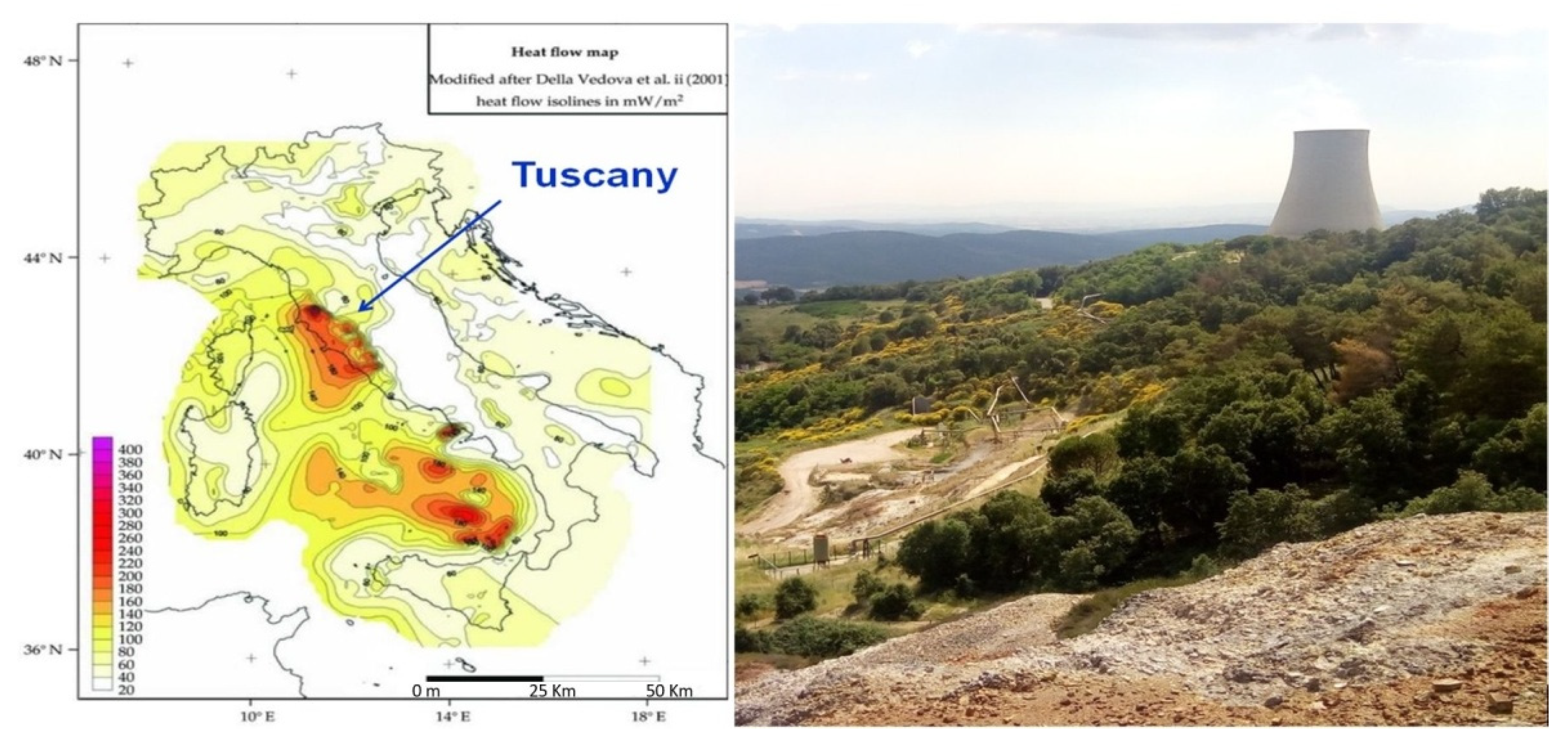
Parco delle Biancane is located in central Italy, in a steam-dominated geothermal field [
25]. The area 1-km-wide and 2-km-long is located near the wide thermal anomaly that affects most of Tuscany region (
Figure 1). In literature there are several works on modeling and measurements of the deep geothermal field [
3,
4,
26,
27], but there is a lack of studies about the characterization of surface thermal signatures that needs to be filled up.
The Larderello–Travale geothermal system, known as Larderello geothermal field (of which Parco delle Biancane is part,
Figure 2), is the site of a large-scale steam-dominated geothermal anomaly. In this area, superheated steam is present at depths over 3.5 km and with temperatures exceeding 350 °C, whereas the deep reservoir of the Mt. Amiata geothermal fields shows a two-phase (liquid + vapor mixture) state with temperatures of 300–350 °C [
1].
The different geological assets and thermal behavior of these areas correspond to surface thermal anomalies that may be very different both for the maximum temperatures and for the size and distribution on the ground. In this context, systematic global recording of thermal anomalies as measured from high spatial resolution space borne sensors [
28] and thermal images acquired by using UAV need to be improved.
2.2. Satellite Data
Cloud-free Landsat 8 thermal infrared sensor (TIRS) images were downloaded from USGS web site [
30]. Satellite data have a spatial resolution of 100 m and provided with a resampling at 30 m.
Table 1 reports the main characteristics of Landsat 8 [
31]. Considering the extension of the test site, thermal anomalies are easily visible from satellite data. For the purpose of this analysis to eliminate temperature measurements inaccuracies due to the solar radiation nighttime Landsat 8 acquisitions of TIRS were considered.
Landsat 8 acquired on 16 June and 27 September 2018 and 19 June 2019 and in order to collect data as simultaneously as possible, surveys were conducted near these dates.
Figure 3 shows how easily the presence of thermal anomaly is detected by remote sensing data.
2.3. Unmanned Aerial Vehicle (UAV) Data Acquisition
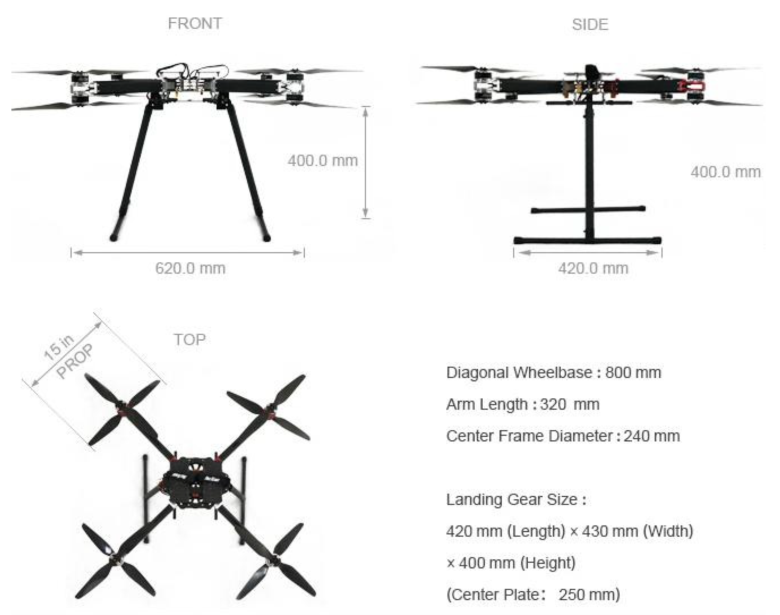
A FlyBit octocopter [
32], showed in
Figure 4, was used to carry out unmanned surveys from UAVs.
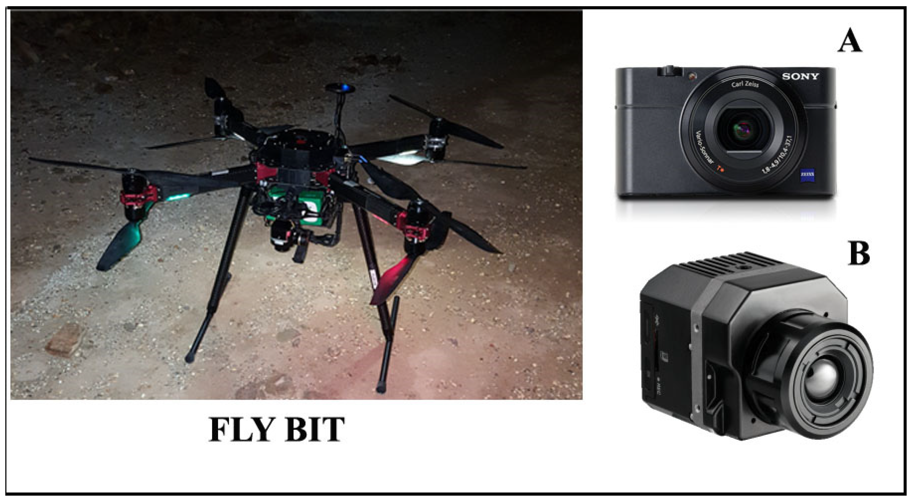
The UAV had a takeoff mass (TOM) of 8.5 kg and was equipped with a FLIR VUE PRO R thermal imaging camera in order to gather thermal infrared measurements; additional a Sony Alpha 6000 camera was also used to collect photogrammetric data (
Figure 5;
Table 2). For both sensors to keep constant orientation, the two devices were stabilized using specific gimbals.
Table 2 shows the technical characteristics of a hand-held thermal camera (FLIR SC640, FLIR Systems Srl, Milan, Italy) used to carry out thermal field measurements and at the same time of flights of the UAV are also reported.
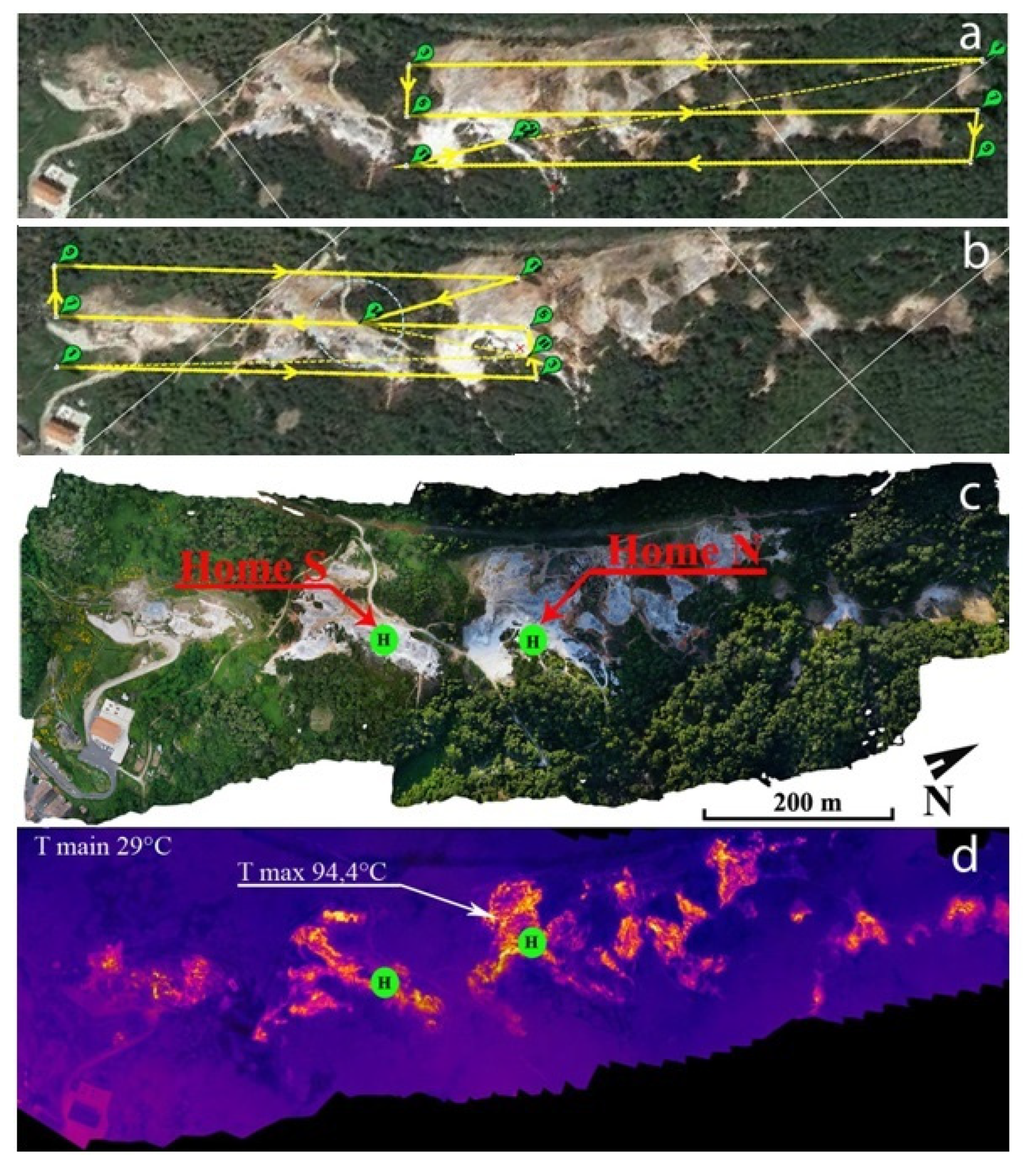
Flight plan was carried out (
Figure 6a) to obtain a good coverage of the investigated area (
Figure 2). Flight plans were always performed in the “scheduled and assisted flight” mode [
32] and were split in two legs as shown in
Figure 6a,b which indicate the northern sector and the southern sector, respectively. The survey area shows a variable morphology with a gently decreasing of elevation passing from North to South sector. Zenithal images were collected by using the single grid option of the autopilot software (mission planner,
Figure 6a) with an 80%–60% overlap between the image footprints (80% in width and 60% in height).
Both flights were performed during nighttime to reduce the effect of solar radiation and to acquire thermal data at an hour close to the night passage of Landsat 8 satellite. Thermal flights were preceded by the acquisition of visible images during daylight hours. In
Figure 6 the UAV acquired visible and thermal images are showed.
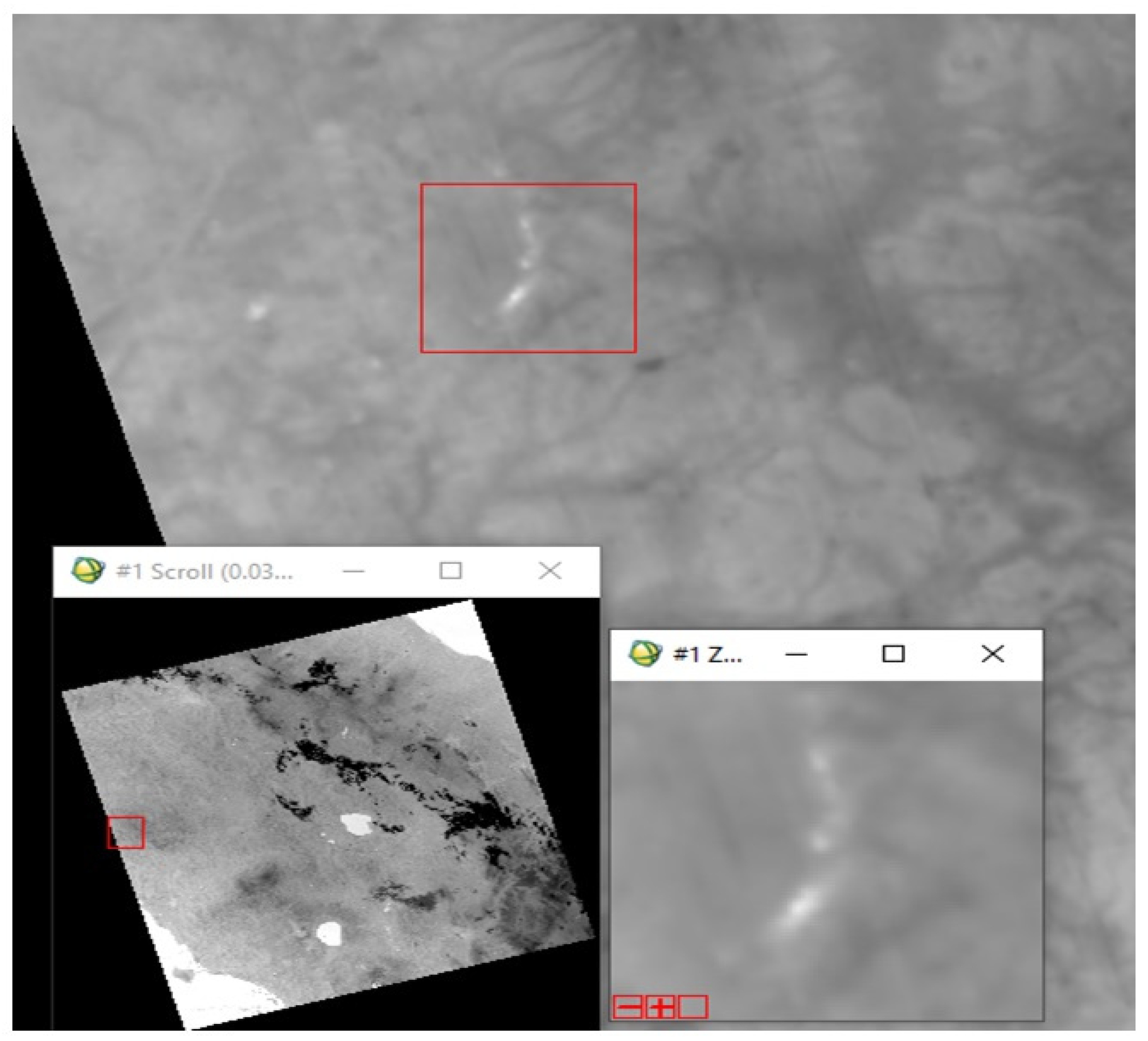
Handheld thermal camera was also used to verify and possible calibrate thermal imagery from the UAV (
Figure 7).
3. Methods
In this work, we applied the procedure proposed by [
33] to detect spatial thermal anomalies and to compare data acquired by satellite with UAV data. Satellite images and UAV data were preprocessed to obtain comparable thermal maps.
The procedure consisted in three main steps: preprocessing of satellite images; preprocessing of UAV images; evaluation and comparison of thermal anomalies in the maps.
3.1. Satellite Image Preprocessing
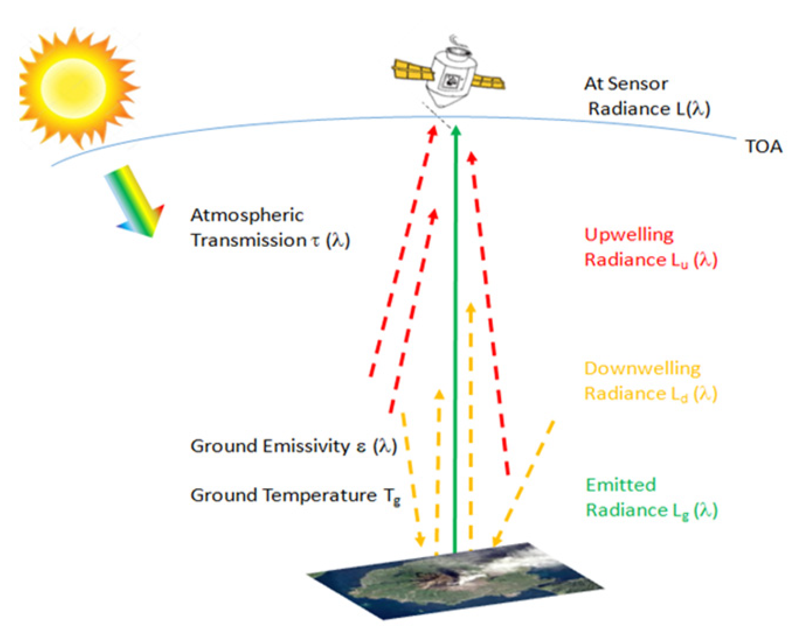
In
Figure 8 the main contributions for estimating the surface temperature are described. The radiance acquired by Landsat 8 is used to evaluate the surface temperature by Planck equation after applying the radiometric calibration to convert the digital number first and the atmospheric corrections later. While the radiometric calibration is obtained following [
31] in terms of Top Of Atmosphere (TOA) radiance, the atmospheric correction is necessary to retrieve the emitted radiance by removing the atmospheric transmission effect and the down welling and upwelling radiances. Considering the well-known moderate spectral resolution transmittance model (MODTRAN, [
34,
35]) for the atmospheric correction, we apply it to remove these effects. Moreover, since the surface emissivity is also an important variable to consider for the surface temperature retrieval, we use the advanced spaceborne thermal emission and reflection radiometer (ASTER) Global Emissivity Dataset (GED) emissivity data downloaded for free by USGS web site [
30]. ASTER-GED land surface temperature and emissivity data products are generated using the ASTER Temperature Emissivity Separation (TES) algorithm with a Water Vapor Scaling (WVS) atmospheric correction method using Moderate Resolution Imaging Spectroradiometer (MODIS) MOD07 atmospheric profiles and the MODTRAN radiative transfer model. This dataset is computed from all clear-sky pixels of ASTER scenes acquired from 2000 through 2008 [
36] and has a spatial resolution of 100 m. The ASTER-GED emissivity around Parco delle Biancane area reaches value around 0.96–0.97 within the 10.6–11.2 μm range.
The surface temperature retrieval is obtained by applying the Radiative Transfer Equation (RTE) of [
37] and inverting the Plank’s law, Equation (1):
where L is the sensor radiance in W m
−2 sr
−1 μm
−1, ε the surface emissivity (in this area the value of ASTER-GED emissivity related to the wavelength 10.89 is around 0.96 and 0.97), λ the considered band wavelength at 10.89 μm (Band 10 of Landsat 8-TIRS),
,
. The retrieved temperature in K is then converted in degree Celsius (°C).
For the validation of the methodology used to estimate the surface temperature by Landsat 8, we refer to [
33,
38]. In [
33] comparative analyses were conducted by using the same procedure for Landsat 8 and fixed thermal camera (TIRNet) installed at Solfatara volcano (near Naples, Italy). The comparison among temperature time series extracted from satellite and TIRNet analysis areas evidenced that temperature estimated by satellite data are reliable to be compared with values extracted from ground measurement provided by TIRNet frames acquired at different spatial scale, used for validation purposes. In [
38], cross-comparison between different satellite sensors on Italian active volcanoes and Parco delle Biancane geothermal area was considered. The Pearson correlation coefficient was analyzed, and considering that a value greater than 0.7 indicates a high correlation, all the temperature fields derived from different sensors in [
38] had a very good correlation. Considering the results achieved in [
33,
38], we are confident on the results obtained in this work.
3.2. UAV Image Preprocessing
Thermal surveys were composed from each set of shots of each flight. The internal software of the FLIR camera allows to correct each thermal shot for the effects of distance, emissivity, atmospheric temperature and relative humidity. The emissivity was set to the value of 0.96 considering the surface conditions and following the value of emissivity used in the Equation (1) for satellite data; the height of the set flight plan was used to set the distance. Temperature and relative humidity were recorded with a thermo-hygrometer before the flight.
The images collected by UAV are processed with bundle adjustment 3D-recostruction algorithm that allows to obtain an orthomosaic. All the reconstructions (both visible and thermal) were performed with the use of the Pix4D software (version 4.4.12) [
39].
The first two thermal flights (in June 2018) were carried out using a constant height of 120 m (
Table 3) so that the orographic changes in the terrain (
Table 3) were not taken into account resulting in real distance of the UAV from the ground being different for each frame. For this reason, the next step was to verify the temperature values as a function of the real distance of the UAV from the ground and thus allowing for the size of the pixel on the ground and the size of the images to vary accordingly. The other thermal flights (in September 2018 and in June 2019) took place keeping different heights in the two sectors (T-N and T-S in
Table 3) resulting in real distance of the UAV from the ground.
Despite this, the temperature data produced can be considered reliable as they were validated by Thermal Cam Research Pro software (version 2.10) [
40], which analyses thermal images and automatically adjusts the values of the individual shots according to the value of the distance (which we did vary according to the topography). Therefore, the average temperature of the individual sectors is the same and the maximum temperature shows a negligible gap of about 0.3 °C.
3.3. Evaluation and Comparison of Thermal Anomalies
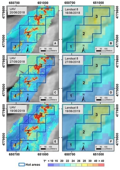
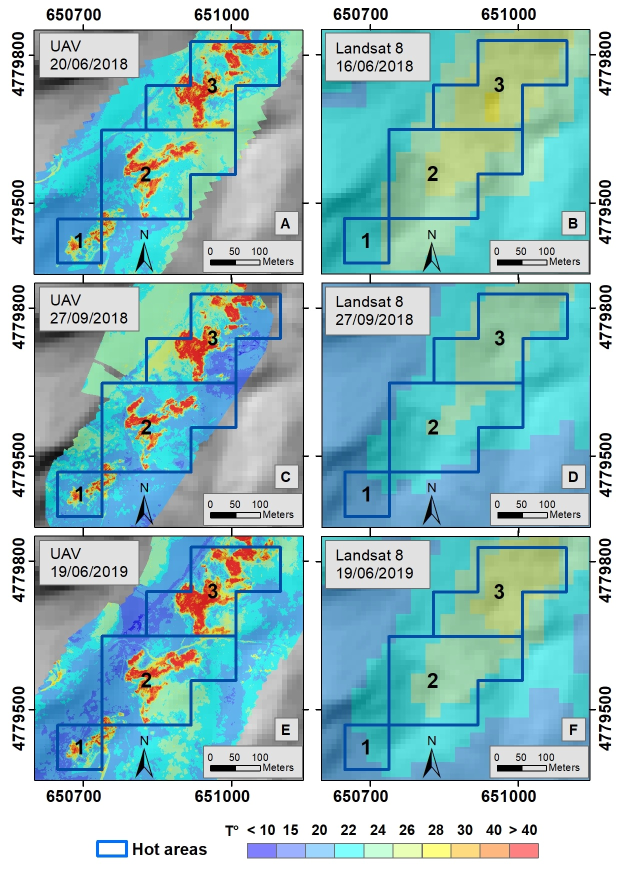
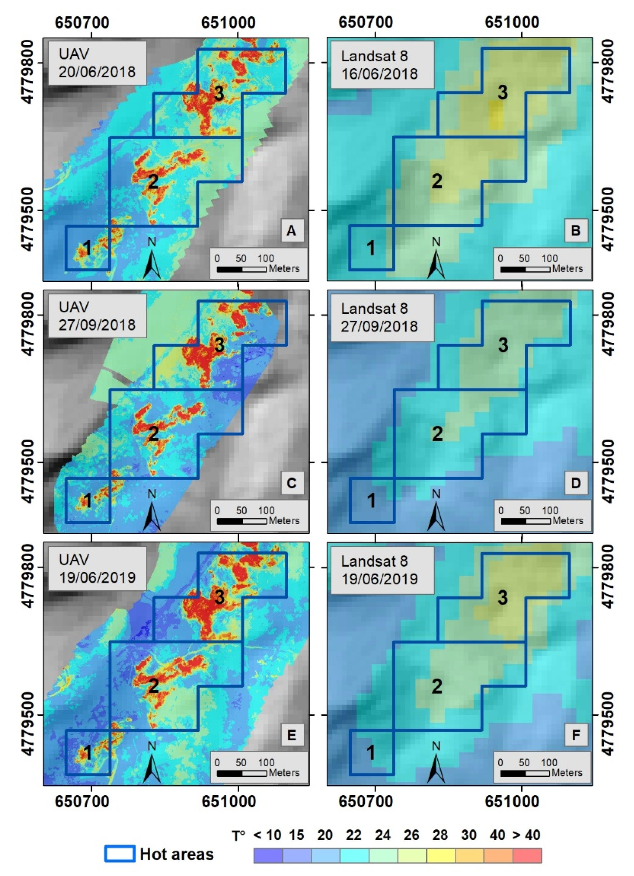
In order to compare spatial thermal anomaly both of UAV and Landsat 8, polygons were set following the regular spaced grid of 30 m × 30 m satellite data. These polygons define the common thermal anomaly, as shown in
Figure 9. Statistical information on the average temperature within the areas of thermal anomaly were obtained using the zonal statistical function (ArcGIS© algorithm [
41]). This algorithm allows to extract the main statistical information as the number of pixels per area, Range (T max–T min), T average and Standard deviation (
Table 4,
Table 5 and
Table 6).
4. Results and Discussion
The flight on 20 June 2018 should be considered as a test flight as it does not coincide with the satellite passage on 16 June. Despite this, a good correspondence between the average temperatures extracted from both UAV and satellite images, within the three areas of identified anomalies, made it possible to plan the subsequent acquisition campaigns for best matching results. The comparison between the data, shown in
Figure 9, made it possible to obtain
Table 4,
Table 5 and
Table 6, where the statistical analysis on temperatures calculated within the three areas of thermal anomaly show a good correspondence between the temperatures acquired by Landsat 8 and those acquired by UAV.
Considering Area 1 in
Figure 9, for all three field campaigns, there is a high correlation of Landsat 8 and UAV average temperatures despite the fact that on June 2018 when the UAV survey was not in sync with the satellite acquisition data. Area 1 is the smallest (about 8100 m
2) and the number of UAV pixels included in this area varies to the different flight heights (from 100 m to 120 m, as reported in
Table 3). Moreover the high spatial resolution of UAV thermal maps offers high accuracy in measurements, in agreement with the high number of pixels, the range and standard deviation reported in
Table 4,
Table 5 and
Table 6.
The same considerations apply to Area 2 (about 40,500 m2): very good agreement with satellite data also considering the high number of UAV pixels covering the area.
With regard to Area 3 (about 32,400 m
2), the UAV survey conducted on September 2018 unfortunately does not cover the same area (
Figure 9c). This resulted in fewer UAV measurements included in this area (
Table 5), missing the cold areas; this could explain the difference of satellite and UAV temperature (22.6 °C, 26.1 °C, respectively).
For all three UAV surface temperature maps, the high variance of temperature range and the standard deviation reported in
Table 4,
Table 5 and
Table 6 demonstrate the strong capacity of the UAV measurements in terms of temperature to obtain very detailed temperature maps.
The next flight missions will not be set at fixed heights from the take-off point but at a constant height with respect to the topography. In other words, once the flight height has been decided, the software allows you to automatically set “follow the morphology”.
Future work will feature flights with crossed grid and variable height according to the topography. Moreover, the calculation of additional thermal parameters like the heat flow and a series of multi-scalar structural geology investigations will be performed with the aim to better understand the relationship between the Parco delle Biancane geothermal district and the tectonic setting of the area. Further lineament analyses will be done on remotely sensed TIR images and, to bridge the outcrop investigation conducted at regional scale, TIR satellite and VIS images acquired by drone will be further investigated.
This multidisciplinary approach will help us to better understand the thermal structure of Parco delle Biancane geothermal area.
5. Conclusions
In this work, we have investigated the main thermal anomalies in Parco delle Biancane area using surface temperature measurements at different resolution scale. The surface temperature was retrieved from Landsat 8 data by removing the atmospheric effects and using, as surface emissivity conditions, the values obtained from ASTER-GED data. To reduce the solar effects, the analysis was conducted using nighttime Landsat 8 data. Moreover, during the three separate surveys, surface temperature was also measured by using a thermal camera mounted on a UAV. Even for the UAV surface temperature retrieval we used a surface emissivity 0.96 in sync with the one used for Landsat 8.
The results of this analysis show a high correlation (
Table 4,
Table 5 and
Table 6) of the average temperatures in the three selected areas.
With this work we are confident that at the spatial resolution of the Landsat 8 satellite images, thermal anomalies are detectable and with the support of UAV surveys detailed information can be obtained. The capability to use remote sensing data for the detection and exploration of geothermal areas is also tested. In particular, the obtained results also confirm that remote sensing data can be used as an important technique for geothermal field analysis thanks to systematic and precise detection of thermal anomalies.
Medium/high spatial resolution thermal range satellite data allow to detect surface thermal anomalies connected to geothermal fields; satellite data could be successfully integrated with low cost techniques by means of UAVs adapted to optimize thermal, geochemical and geomorphologic measurements in selected sites.
UAV survey is well-suited for targeted geothermal monitoring: it enables to estimate surface temperature without the need to apply atmospheric correction and using higher spatial resolution images compared to the satellite. At the same time, satellite imagery provides the best solution for larger areas.
A future development of this work will be to analyze time series of satellite thermal data using Landsat 8, ASTER thermal data (90 m pixel spatial resolution) and the last ECOSTRESS (ecosystem spaceborne thermal radiometer experiment on space station (69 m × 38 m pixel spatial resolution at nadir), in order to observe changes in the surface temperatures in the active geothermal areas.
Author Contributions
Conceptualization, M.S., E.M. and M.F.B.; data curation, M.S., E.B.S., T.C.; methodology, S.T.; data UAV elaboration, P.B., G.A.; UAV assistance, V.D.L. and V.L.; writing—review & editing, all. All authors have read and agreed to the published version of the manuscript.
Funding
This research was funded by the INGV-FISR 2016 Fondo integrativo speciale per la ricerca (FISR): Riparto per gli anni 2015 e 2016 a progetti di ricerca (Delibera CIPE n. 71/2016) per l’INGV: “Centro di studio e monitoraggio dei rischi naturali dell’Italia Centrale”.
Acknowledgments
Landsat 8 L1T processing, archiving and distribution are performed by the USGS. The Assessors of Monte Rotondo Marittimo for the free access and logistical support at Parco delle Biancane (Pippucci Orano and Emy Macrini). Thanks to Laboratorio di Geologia e Geotecnica of Istituto Nazionale di Geofisica e Vulcanologia and Luca Pizzimenti for the collaboration offered in the retrieval of TINTALY digital elevation model. A special thanks to Federico Rabuffi for his help in
Figure 2 and Massimo Musacchio and Vito Romaniello for their precious suggestions. Thanks are extended to Alexander Shaw and his wife Serena Tramonti for checking the English. The authors wish to thank the three reviewers for their constructive comments.
Conflicts of Interest
The authors declare no conflict of interest.
References
- Barelli, A.; Ceccarelli, A.; Dini, I.; Fiordelisi, A.; Giorgi, N.; Lovari, F.; Romagnoli, P. A review of the Mt. Amiata geothermal system (Italy). In Proceedings of the World Geothermal Congress, Bali, Indonesia, 25–29 April 2010; pp. 1–4. [Google Scholar]
- Gianelli, G. A comparative analysis of the geothermal fields of Larderello and Mt Amiata, Italy. In Geothermal Energy Research Trends; Ueckerman, H.I., Ed.; Nova Science Publishers Inc.: New York, NY, USA, 2008; pp. 59–85. ISBN 1-60021-683-8. [Google Scholar]
- Batini, F.; Brogi, A.; Lazzarotto, A.; Liotta, D.; Pandeli, E. Geological features of Larderello-Travale and Mt. Amiata geothermal areas (southern Tuscany, Italy). Episodes 2003, 26, 239–244. [Google Scholar] [CrossRef] [PubMed]
- Bellani, S.; Brogi, A.; Lazzarotto, A.; Liotta, D.; Ranalli, G. Heat flow, deep temperatures and extensional structures in the Larderello Geothermal Field (Italy): Constraints on geothermal fluid flows. J. Volcanol. Geotherm. Res. 2004, 132, 15–29. [Google Scholar] [CrossRef]
- Bellani, S.; Magro, G.; Brogi, A.; Lazzarotto, A.; Liotta, D. Insights into the Larderello geothermal field: Structural setting and distribution of thermal and 3He anomalies. In Proceedings of the World Geothermal Congress, Antalya, Turkey, 24–29 April 2005; Volume 2429. [Google Scholar]
- Chiodini, G.; Avino, R.; Caliro, S.; Minopoli, C. Temperature and pressure gas geoindicators at the Solfatara fumaroles (Campi Flegrei). Ann. Geophys. 2011, 54, 151–160. [Google Scholar]
- Ramírez-González, L.M.; Aufaristama, M.; Jónsdóttir, I.; Höskuldsson, Á.; Proietti, N.M.; Kraft, G.; McQuilkin, J. Remote sensing of surface Hydrothermal Alteration, identification of Minerals and Thermal anomalies at Sveifluháls-Krýsuvík high-Temperature Geothermal field, SW Iceland. In Earth and Environmental Science, Proceedings of the 7th ITB International Geothermal Workshop 2018, Bandung, Indonesia, 21–22 March 2018; IOP Publishing: Bristol, UK, 2019; Volume 254, No. 1; p. 012005. [Google Scholar]
- García-Santos, V.; Cuxart, J.; Jiménez, M.A.; Martínez-Villagrasa, D.; Simó, G.; Picos, R.; Caselles, V. Study of Temperature Heterogeneities at Sub-Kilometric Scales and Influence on Surface–Atmosphere Energy Interactions. Trans. Geosci. Remote. Sens. 2018, 57, 640–654. [Google Scholar] [CrossRef]
- Nishar, A.; Richards, S.; Breen, D.; Robertson, J.; Breen, B. Thermal infrared imaging of geothermal environments and by an unmanned aerial vehicle (UAV): A case study of the Wairakei–Tauhara geothermal field, Taupo, New Zealand. Renew. Energy 2016, 86, 1256–1264. [Google Scholar] [CrossRef]
- Cherkasov, S.V.; Farkhutdinov, A.M.; Rykovanov, D.P.; Shaipov, A.A. The Use of Unmanned Aerial Vehicle for Geothermal Exploitation Monitoring: Khankala Field Example. J. Sustain. Dev. Energy Water Environ. Syst. 2018, 6, 351–362. [Google Scholar] [CrossRef] [Green Version]
- Settle, M. Workshop on Geological Applications of Thermal Infrared Remote Sensing Techniques: A Lunar and Planetary Institute Workshop; Settle; Lunar and Planetary Institute: Houston, XT, USA, 1980. [Google Scholar]
- Zhou, Y. The application of thermal infrared remote sensing techniques in geothermal surveying. Remote Sens. Land Resour. 1998, 4, 24–28. [Google Scholar]
- Lee, K. Analysis of thermal infrared imagery of the Black Rock Desert geothermal area. Q. Colo. Sch. Mines 1978, 73. [Google Scholar]
- Hellman, M.J.; Ramsey, M.S. Analysis of hot springs and associated deposits in Yellowstone National Park using ASTER and AVIRIS remote sensing. J. Volcanol. Geotherm. Res. 2004, 135, 195–219. [Google Scholar] [CrossRef]
- Vaughan, R.G.; Hook, S.J.; Calvin, W.M.; Taranik, J.V. Surface mineral mapping at Steamboat Springs, Nevada, USA, with multi-wavelength thermal infrared images. Remote Sens. Environ. 2005, 99, 140–158. [Google Scholar] [CrossRef]
- Coolbaugh, M.F.; Kratt, C.; Fallacaro, A.; Calvin, W.M.; Taranik, J.V. Detection of geothermal anomalies using advanced spaceborne thermal emission and reflection radiometer (ASTER) thermal infrared images at Bradys Hot Springs, Nevada, USA. Remote Sens. Environ. 2007, 106, 350–359. [Google Scholar] [CrossRef]
- Watson, F.G.; Lockwood, R.E.; Newman, W.B.; Anderson, T.N.; Garrott, R.A. Development and comparison of Landsat radiometric and snowpack model inversion techniques for estimating geothermal heat flux. Remote Sens. Environ. 2008, 112, 471–481. [Google Scholar] [CrossRef]
- Williams, R.S., Jr. The use of broadband thermal infrared images to monitor and to study dynamic geological phenomena. In Geological Applications of Thermal Infrared Remote Sensing Techniques; Settle; Lunar and Planetary Institute: Houston, XT, USA, 1981; p. 98. [Google Scholar]
- Lago, G.D.; Rodríguez-Gonzálvez, P. Detection of Geothermal Potential Zones Using Remote Sensing Techniques. Remote. Sens. 2019, 11, 2403. [Google Scholar] [CrossRef] [Green Version]
- Howari, F. Prospecting for geothermal energy through satellite based thermal data: Review and the way forward. Glob. J. Environ. Sci. Manag. 2015, 1, 265–274. [Google Scholar]
- Abubakar, A.J.A.; Hashim, M.; Pour, A.B.; Shehu, K. A review of geothermal mapping techniques using remotely sensed data. Sci. World J. 2017, 12, 72–82. [Google Scholar]
- Avtar, R.; Sahu, N.; Aggarwal, A.K.; Chakraborty, S.; Kharrazi, A.; Yunus, A.P.; Dou, J.; Kurniawan, T.A. Exploring Renewable Energy Resources Using Remote Sensing and GIS—A Review. Resources 2019, 8, 149. [Google Scholar] [CrossRef] [Green Version]
- Fridleifsson, I.B.; Bertani, R.; Huenges, E.; Lund, J.W.; Ragnarsson, A.; Rybach, L. The possible role and contribution of geothermal energy to the mitigation of climate change. In Proceedings of the IPCC Scoping Meeting on Renewable Energy Sources, Lübeck, Germany, 20–25 January 2008; pp. 59–80. [Google Scholar]
- Qin, Q.; Zhang, N.; Nan, P.; Chai, L. Geothermal area detection using Landsat ETM+ thermal infrared data and its mechanistic analysis—A case study in Tengchong, China. Int. J. Appl. Earth Obs. Geoinf. 2011, 13, 552–559. [Google Scholar] [CrossRef]
- Saccorotti, G.; Piccinini, D.; Zupo, M.; Mazzarini, F.; Chiarabba, C.; Agostinetti, N.P.; Licciardi, A.; Bagagli, M. The deep structure of the Larderello-Travale geothermal field (Italy) from integrated, passive seismic investigations. Energy Procedia 2014, 59, 227–234. [Google Scholar] [CrossRef]
- Di Filippo, M.; Lombardi, S.; Nappi, G.; Reimer, G.M.; Renzulli, A.; Toro, B. Volcano-tectonic structures, gravity and helium in geothermal areas of Tuscany and Latium (Vulsini volcanic district), Italy. Geothermics 1999, 28, 377–393. [Google Scholar] [CrossRef]
- Della, V.B.; Vecellio, C.; Bellani, S.; Tinivella, U. Thermal modelling of the Larderello geothermal field (Tuscany, Italy). Int. J. Earth Sci. 2008, 97, 317–332. [Google Scholar] [CrossRef]
- Buongiorno, M.F.; Pieri, D.; Silvestri, M. Thermal Analysis of Volcanoes Based on 10 Years of ASTER Data on Mt. Etna. In Thermal Infrared Remote Sensing Remote Sensing and Digital Image Processing; Springer: Dordrecht, The Netherlands, 2013; Volume 17, pp. 409–428. [Google Scholar]
- Della, V.B.; Bellani, S.; Pellis, G.; Squarci, P. Deep temperatures and surface heat flow distribution. In Anatomy of an Orogen: The Apennines and Adjacent Mediterranean Basins; Springer: Dordrecht, The Netherlands, 2001; pp. 65–76. [Google Scholar]
- USGS Data Provider. Available online: https://earthexplorer.usgs.gov/ (accessed on 5 March 2020).
- Landsat 8 Data User Handbook. Available online: https://www.usgs.gov/media/files/landsat-8-data-users-handbook (accessed on 5 March 2020).
- Marotta, E.; Avvisati, G.; Belviso, P.; Carandente, A.; Peluso, R.; Sansivero, F.; Vilardo, G.; Sangianantoni, A.; Santiccioli, G.; Sacchetta, E.; et al. Gestione Operativa dei SAPR OV-INGV per Monitoraggio e Ricerca; INGV Rapporti Tecnici; Rome, Italy, 2017; p. 365. ISSN 2039-7941. [Google Scholar]
- Caputo, T.; Bellucci Sessa, E.; Silvestri, M.; Buongiorno, M.F.; Musacchio, M.; Sansivero, F.; Vilardo, G. Surface temperature multiscale monitoring by thermal infrared satellite and ground images at Campi Flegrei volcanic area (Italy). Remote Sens. 2019, 11, 1007. [Google Scholar] [CrossRef] [Green Version]
- Berk, A.; Conforti, P.; Kennett, R.; Perkins, T.; Hawes, F.; van den Bosch, J. MODTRAN6: A Major Upgrade of the MODTRAN Radiative Transfer Code. Available online: https://www.spiedigitallibrary.org/conference-proceedings-of-spie/9088/1/MODTRAN6--a-major-upgrade-of-the-MODTRAN-radiative-transfer/10.1117/12.2050433.short?SSO=1 (accessed on 10 June 2020). [CrossRef]
- Berk, A.; Conforti, P.; Hawes, F. An accelerated line-By-Line option for MODTRAN combining on-The-Fly generation of line center absorption with 0.1 cm-1 bins and pre-computed line tails. Available online: https://www.spiedigitallibrary.org/conference-proceedings-of-spie/9472/1/An-accelerated-line-by-line-option-for-MODTRAN-combining-on/10.1117/12.2177444.short (accessed on 10 June 2020). [CrossRef]
- Advanced Spaceborne Thermal Emission and Reflection Radiometer. Global Emissivity Dataset GED. Available online: https://lpdaac.usgs.gov/products/ag100v003/ (accessed on 5 March 2020).
- Barsi, J.A.; Barker, J.L.; Schott, J.R. An Atmospheric Correction Parameter Calculator for a single thermal band earth-sensing instrument. In Proceedings of the 2003 IEEE International Geoscience and Remote Sensing Symposium, Toulouse, France, 21–25 July 2003; Volume 5, pp. 3014–3016. [Google Scholar]
- Silvestri, M.; Romaniello, V.; Hook, S.; Musacchio, M.; Teggi, S.; Buongiorno, M.F. First Comparisons of Surface Temperature Estimations between ECOSTRESS, ASTER and Landsat 8 over Italian Volcanic and Geothermal Areas. Remote Sens. 2020, 12, 184. [Google Scholar] [CrossRef] [Green Version]
- Pix4DMapper User Manual. Available online: https://support.pix4d.com/hc/en-us/sections/360003718992-Manual (accessed on 20 March 2020).
- Thermal Camera. Available online: https://www.imveurope.com/press-releases/thermacam-researcher-v210 (accessed on 20 March 2020).
- ESRI. ArcGIS Desktop: Release 10; Environmental Systems Research Institute, Inc.: Redlands, CA, USA, 2011. [Google Scholar]
- Tarquini, S.; Isola, I.; Favalli, M.; Mazzarini, F.; Bisson, M.; Pareschi, M.T.; Boschi, E. TINITALY/01: A New Triangular irRegular Network of Italy. Ann. Geophys. 2007, 50, 407–425. [Google Scholar]
- Tarquini, S.; Vinci, S.; Favalli, M.; Doumaz, F.; Fornaciai, A.; Nannipieri, L. Release of a 10-m-resolution DEM for the Italian territory: Comparison with global-Coverage DEMs and anaglyph-mode exploration via the web. Comput. Geosci. 2012, 38, 168–170. [Google Scholar] [CrossRef] [Green Version]
- Tarquini, S.; Nannipieri, L. The 10 m-resolution TINITALY DEM as a trans-disciplinary basis for the analysis of the italian territory: Current trends and new perspectives. Geomorphology 2017, 281, 108–115. [Google Scholar] [CrossRef]
Figure 1.
Heat flow distribution (modified after [
29]) and cooling towers near Parco delle Biancane site.
Figure 1.
Heat flow distribution (modified after [
29]) and cooling towers near Parco delle Biancane site.
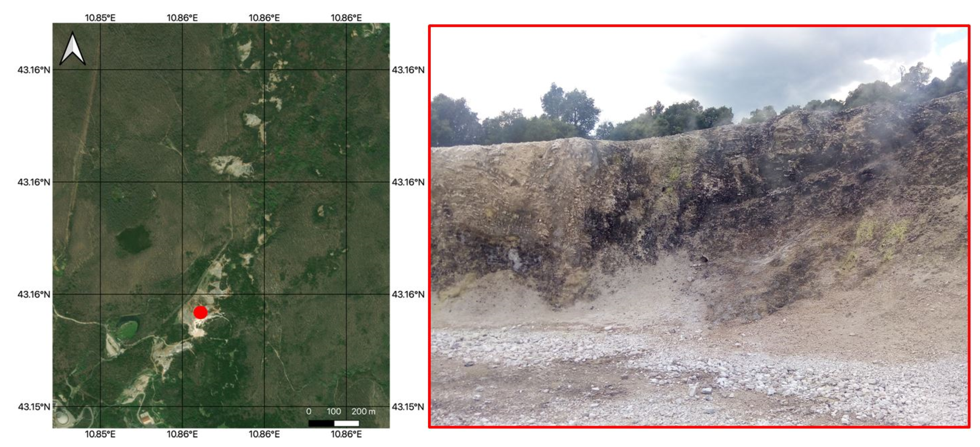
Figure 2.
Test site: left, Parco delle Biancane (Monterotondo Marittimo, Grosseto, Italy); right, presence of fumaroles in the test site (in red the position on the map of the collected picture).
Figure 2.
Test site: left, Parco delle Biancane (Monterotondo Marittimo, Grosseto, Italy); right, presence of fumaroles in the test site (in red the position on the map of the collected picture).
Figure 3.
Landsat 8 TIRS 10 band. In the red box the investigated area.
Figure 3.
Landsat 8 TIRS 10 band. In the red box the investigated area.
Figure 4.
FlyBit octocopter and main features.
Figure 4.
FlyBit octocopter and main features.
Figure 5.
FlyBit octocopter and equipment. (A) Sony Alpha 6000 camera; (B) FLIR VUE PRO R thermal imaging camera.
Figure 5.
FlyBit octocopter and equipment. (A) Sony Alpha 6000 camera; (B) FLIR VUE PRO R thermal imaging camera.
Figure 6.
UAV flight of 19 June 2019 on the Parco delle Biancane: (a) flight plan for the northern sector; (b) flight plane for the southern sector; (c) visible mapping; (d) thermal mapping. The “Home” (H) indicates the take-off point of the UAV which has a ground elevation of 621 m and 610 m in the northern and southern sector, respectively.
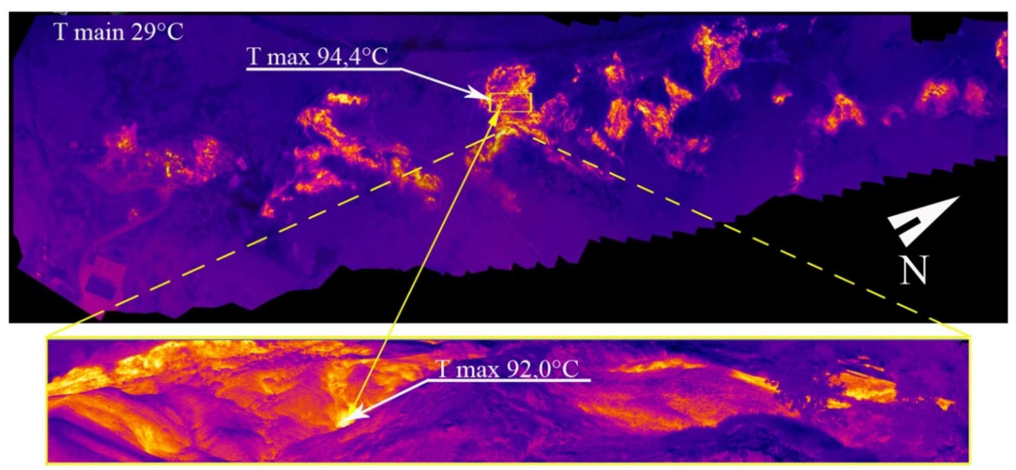
Figure 7.
Thermal mapping from UAV flight (above) and from hand-held thermal camera (below) of 19 June 2019 on the Parco delle Biancane.
Figure 7.
Thermal mapping from UAV flight (above) and from hand-held thermal camera (below) of 19 June 2019 on the Parco delle Biancane.
Figure 8.
Atmospheric correction to surface temperature estimation.
Figure 8.
Atmospheric correction to surface temperature estimation.
Figure 9.
Maps of land surface temperature of UAV (
A,
C,
E) and Landsat 8 (
B,
D,
F) over the TINITALY digital elevation model [
42,
43,
44].
Figure 9.
Maps of land surface temperature of UAV (
A,
C,
E) and Landsat 8 (
B,
D,
F) over the TINITALY digital elevation model [
42,
43,
44].
Table 1.
Main characteristics of Landsat 8.
Table 1.
Main characteristics of Landsat 8.
| Characteristics | Description |
|---|
Launch date
Orbit | 11 February 2013Worldwide reference system -2 (WRS-2) path/row system Sun-synchronous orbit at an altitude of 705 km 233 orbit cycle; covers the entire globe every 16 days (except for the highest polar latitudes) Inclined 98.2° Circles the Earth every 98.9 min Equatorial crossing time: 10:00 a.m. +/− 15 min
|
| Scenes/day | ~700 |
Scene size
TIRS sensor | 190 km × 180 km
10.60–11.19 μm (TIRS 10)
11.50–12.51 μm (TIRS 11) |
| TIRS sensor spatial resolution | 100 m |
| TIRS noise equivalent change in temperature (NEΔT) | TIRS10: 0.069(NEDT@240), 0.053(NEDT@280), 0.046(NEDT@320), 0.043(NEDT@360)
TIRS11: 0.079(NEDT@240), 0.059(NEDT@280), 0.049(NEDT@320), 0.045(NEDT@360) |
| Landsat 8 nighttime acquisitions for this work | 16 June 2018
27 September 2018
19 June 2019 |
Table 2.
Main technical specifications of sensors: FLIR VUE PRO (unmanned aerial vehicle (UAV) thermal cam); SONY ALFPHA 6000 (UAV visible-cam); FLIR SC 640 (hand-held thermal camera).
Table 2.
Main technical specifications of sensors: FLIR VUE PRO (unmanned aerial vehicle (UAV) thermal cam); SONY ALFPHA 6000 (UAV visible-cam); FLIR SC 640 (hand-held thermal camera).
| FLIR VUE PRO | SONY ALPHA 6000 | FLIR SC 640 |
|---|
| Overview: | Sensor: | Imaging Performance: |
| Thermal imager: uncooled VOx microbolometer | Max resolution: 6000 × 4000 | Field of view (FOV)/minimum focus distance: 24° × 18°/0.3 m |
| Resolution: 640 × 512 | Effective pixel: 24 megapixels | Spatial resolution: 0.65 mrad for 24°lens |
| Lens: 9 mm; 69° × 56° | Sensor size: APS-C (23.5 × 15.6 mm) | Thermal sensitivity: 30 mK at 30 °C |
| Spectral band: 7.5–13.5 μm | Processor: Bionz X | Electronic zoom: 1–8× continuous including pan function |
| Full frame rates: 30 Hz (NTSC); 25 Hz (PAL) | Image: | Electric and manual focus with USM technology: Auto and Manual |
| Exportable frame rates: 7.5 Hz (NTSC); 8.3 Hz (PAL) | ISO: auto, 100–25,600 (51,200 with Multi-Frame NR) | Measurement: |
| Environmental: | White balance presets: 10 | Accuracy: ±2 °C or ±2% of reading |
| Operating temperature Range: −20 °C to +50 °C | Custom white balance: yes | Temperature range: −40 °C to +1500 °C |
| Non-operating temperature range: −55 °C to +95 °C | Image stabilization: NO | Imaging Performance: |
| Operational altitude: +40,000 feet | Uncompressed format: RAW | IR resolution: 640 × 480 pixels |
| | File format: JPEG (DCF v2.0, EXIF v2.3); RAW (Sony ARW 2.3). | Spectral range: 7.5–13 µm |
| | Optics & Focus: | Image frequency: Up to 120 Hz by windowing |
| | Digital zoom: yes (2×) | Focus: automatic or manual |
| | Manual focus: yes | Focal plane array (FPA): uncooled microbolometer |
| | Videography features: | Image storage: |
| | Format: MPEG-4, AVCHD | Format: standard JPEG—including measurement data |
Table 3.
Date of each measurement campaign; the type of flight if visible (V) or thermal (T) and relative sector of flight (N = North; S = South); the flight height and the relative parameters of the image that is pixel, horizontal field of view (FH), vertical field of view (FV), range of ground elevation, number of pictures and flight duration.
| Date | Type of Flight Sector of Flight | Flight Height (m) | Pixel Size at Ground (cm) | FH (m) | FV (m) | Ground Elevation (m ASL) | N° Images | Flight Duration (Min) |
|---|
| 20 June 2018 | V–N | 110 | 2.2 | 129.3 | 85.8 | 611–658 | 105 | 15:58 |
| 20 June 2018 | V–S | 110 | 2.2 | 129.3 | 85.8 | 537–644 | 78 | 10:38 |
| 20 June 2018 | T–N | 120 | 22.7 | 145.1 | 116.1 | 606–660 | 47 | 07:28 |
| 20 June 2018 | T–S | 120 | 22.7 | 145.1 | 116.1 | 534–631 | 58 | 08:38 |
| 27 September 2018 | T–N | 150 | 28.3 | 181.3 | 145.1 | 602–695 | 59 | 09:10 |
| 27 September 2018 | T–S | 120 | 22.7 | 145.1 | 116.1 | 514–664 | 41 | 08:28 |
| 19 June 2019 | T–N | 120 | 22.7 | 145.1 | 116.1 | 597–691 | 164 | 22:01 |
| 19 June 2019 | T–S | 100 | 18.9 | 120.9 | 96.7 | 531–633 | 214 | 23:03 |
Table 4.
Statistical analysis for June 2018.
Table 4.
Statistical analysis for June 2018.
| Area | T Mean °C | STD | Range | Pixels | Data and Time |
|---|
| 1 | 21.9 | 0.30 | 0.77 | 9 | Landsat 8
16 June 2018 20:52 UTC |
| 2 | 23.8 | 1.03 | 4.25 | 45 |
| 3 | 25.01 | 0.89 | 3.24 | 36 |
| 1 | 21.3 | 5.49 | 56.79 | 99,623 | UAV
20 June 2018 22:25 UTC |
| 2 | 23.7 | 6.81 | 67.79 | 495,654 |
| 3 | 26.42 | 9.55 | 64.02 | 398,500 |
Table 5.
Statistical analysis for September 2018.
Table 5.
Statistical analysis for September 2018.
| Area | T Mean °C | STD | Range | Pixels | Data and Time |
|---|
| 1 | 20.00 | 0.12 | 0.43 | 9 | Landsat 8
27 September 2018 20:59 UTC |
| 2 | 21.3 | 0.75 | 2.91 | 45 |
| 3 | 22.6 | 0.63 | 2.37 | 36 |
| 1 | 21.4 | 5.93 | 63.40 | 107,584 | UAV
27 September 2018 22:30 UTC |
| 2 | 22.2 | 8.44 | 89.35 | 520,636 |
| 3 | 26.1 | 12.69 | 79.04 | 402,738 |
Table 6.
Statistical analysis for June 2019.
Table 6.
Statistical analysis for June 2019.
| Area | T Mean °C | STD | Range | Pixels | Data and Time |
|---|
| 1 | 20.3 | 0.31 | 1.10 | 9 | Landsat 8
19 June 2019 20:53 UTC |
| 2 | 22.3 | 0.81 | 3.50 | 45 |
| 3 | 24.3 | 1.11 | 4.26 | 36 |
| 1 | 19.8 | 6.41 | 58.12 | 152,100 | UAV
19 June 2019 20:52 UTC |
| 2 | 22.6 | 8.57 | 71.40 | 762,451 |
| 3 | 26.7 | 12.98 | 77.71 | 608,790 |
© 2020 by the authors. Licensee MDPI, Basel, Switzerland. This article is an open access article distributed under the terms and conditions of the Creative Commons Attribution (CC BY) license (http://creativecommons.org/licenses/by/4.0/).

 ,
, 


